[SGM Geometric Brownian Motion]

Description:

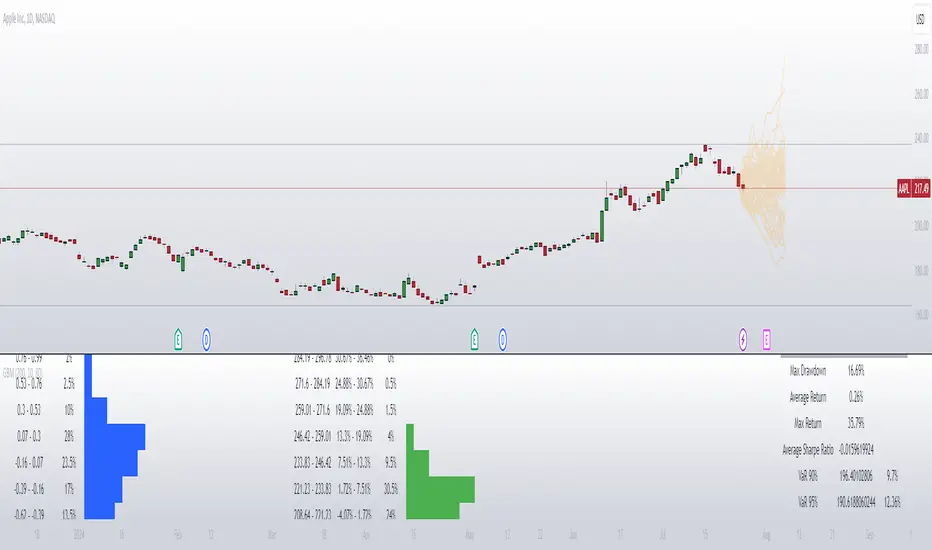
This indicator uses Geometric Brownian Motion (GBM) simulations to predict possible price trajectories of a financial asset. It helps traders visualize potential price movements, assess risks, and make informed decisions.

Geometric Brownian Motion:

Geometric Brownian Motion is an extension of standard Brownian motion (or Wiener process) used to model the random behavior of particles in physics. In finance, this concept is used to model the evolution of asset prices over time in a continuous manner. The basic idea is that the price of an asset does not only change randomly but also exponentially depending on certain parameters.

Basic formula
The formula for the evolution of the price of an asset S(t) under MBG is given by the following stochastic differential equation:

𝑑𝑆(𝑡) = 𝜇𝑆(𝑡)𝑑𝑡 + 𝜎𝑆(𝑡)𝑑𝑊(𝑡)

where:

S(t) is the price of the asset at time

μ is the expected growth rate (or drift).

σ is the volatility of the price of the asset.

dW(t) represents the noise term, i.e. the standard Brownian motion.
Explanations of the terms

Expected growth rate (μ):

This is the expected average return on the asset. If you think your asset will grow by 5% per year,
μ will be 0.05.
Volatility (σ):

It is a measure of the uncertainty or risk associated with the asset. If the asset price varies a lot, σ will be high.

Noise term (dW(t)):

It represents the randomness of the price change, modeled by a Wiener process.

Features:

Customizable number of simulations: Choose the number of price trajectories to simulate to get a better estimate of future movements.
Adjustable simulation length: Set the duration of the simulations in number of periods to adapt the indicator to your trading horizons.
Trajectory display: Visualize the simulated price trajectories directly on the chart to better understand possible future scenarios.
Dispersion calculations: Display the distribution of simulated final prices to assess dispersion and potential variations.
Sharpe ratio distribution: Analyze the risk-adjusted performance of simulations using the Sharpe ratio distribution.
Risk Statistics: Get key risk metrics like maximum drawdown, average return, and Value at Risk (VaR) at different confidence levels.

User Inputs:

Number of Simulations: 200 by default.
Simulation Length: 10 periods by default.
Brownian Motion Transparency: Adjust the transparency of simulated lines for better visualization.
Brownian Motion Display: Enable or disable the display of simulated paths.
Brownian Dispersion Display: Display the distribution of simulated final prices.
Sharpe Dispersion Display: Display the distribution of Sharpe ratios.
Customizable Colors: Choose colors for lines and tables.

Usage:

Configure Settings: Adjust the number of simulations, simulation length, and display preferences to suit your needs.
Analyze Simulated Paths: Simulated path lines appear on the chart, representing possible price developments.
Review Dispersion Charts: Review the charts to understand the distribution of final prices and Sharpe ratios, as well as key risk statistics. This indicator is ideal for traders looking to anticipate future price movements and assess the associated risks. With its detailed simulations and dispersion analyses, it provides valuable insight into the financial markets.