Combined EMA, SMMA, and 60-Day Cycle Indicator V2What This Script Does:
This script is designed to help traders visualize market trends and generate trading signals based on a combination of moving averages and price action. Here's a breakdown of its components and functionality:
Moving Averages:
EMAs (Exponential Moving Averages): These are indicators that smooth out price data to help identify trends. The script uses several EMAs:
200 EMA: A long-term trend indicator.
400 EMA: An even longer-term trend indicator.
55 EMA: A medium-term trend indicator.
89 EMA: Another medium-term trend indicator.
SMMA (Smoothed Moving Average): Similar to EMAs but with different smoothing. The script calculates:
21 SMMA: Short-term smoothed average.
9 SMMA: Very short-term smoothed average.
Cycle High and Low:
60-Day Cycle: The script looks back over the past 60 days to find the highest price (cycle high) and the lowest price (cycle low). These are plotted as horizontal lines on the chart.
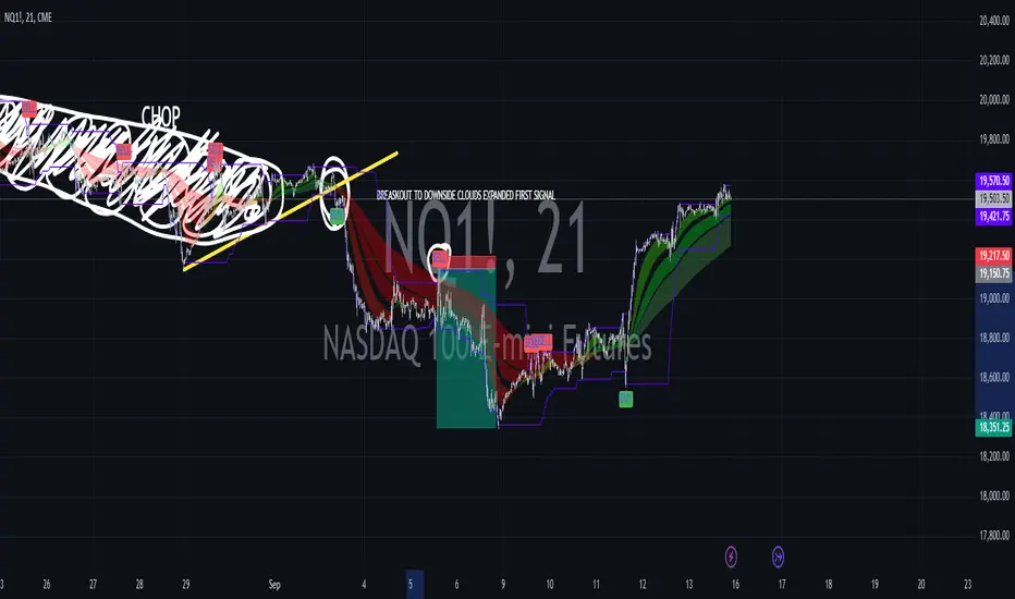
Color-Coded Clouds:
Clouds: The script fills the area between certain EMAs with color-coded clouds to visually indicate trend conditions:
200 EMA vs. 400 EMA Cloud: Green when the 200 EMA is above the 400 EMA (bullish trend) and red when it’s below (bearish trend).
21 SMMA vs. 9 SMMA Cloud: Orange when the 21 SMMA is above the 9 SMMA and green when it’s below.
55 EMA vs. 89 EMA Cloud: Light green when the 55 EMA is above the 89 EMA and red when it’s below.
Trading Signals:
Buy Signal: This is shown when:
The price crosses above the 60-day low and
The EMAs indicate a bullish trend (e.g., the 200 EMA is above the 400 EMA and the 55 EMA is above the 89 EMA).
Sell Signal: This is shown when:
The price crosses below the 60-day high and
The EMAs indicate a bearish trend (e.g., the 200 EMA is below the 400 EMA and the 55 EMA is below the 89 EMA).
How It Helps Traders:
Trend Visualization: The colored clouds and EMA lines help you quickly see whether the market is in a bullish or bearish phase.
Trading Signals: The script provides clear visual signals (buy and sell labels) based on specific market conditions, helping you make more informed trading decisions.
In summary, this script combines several tools to help identify market trends and provide buy and sell signals based on price action relative to a 60-day high/low and the positioning of moving averages. It’s a useful tool for traders looking to visualize trends and automate some aspects of their trading strategy.
Pine Script®指标