Dynamic Volatility Heatmap (ATR)How the Script Works
Dynamic Thresholds:
atrLow and atrHigh are calculated as percentiles (20% and 80% by default) of ATR values over the last double the ATR period (28 days if ATR is 14).
This creates thresholds that adapt to recent market conditions.
Background Heatmap:
Green: ATR is below the low threshold, indicating calm markets (options are cheap).
Red: ATR is above the high threshold, signaling elevated volatility (options are expensive).
Yellow: ATR is within the normal range, showing neutral market conditions.
Overlay Lines:
]Dynamic lines for atrLow and atrHigh help visualize thresholds on the chart.
Interpretation for Trading
Green Zone (Low ATR):
Interpretation: The market is calm, and options are likely underpriced.
Trade Setup: Favor buying options (e.g., long straddles or long calls/puts) to profit from potential volatility increases.
Red Zone (High ATR):
Interpretation: The market is volatile, and options are likely overpriced.
Trade Setup: Favor selling options (e.g., credit spreads or iron condors) to benefit from volatility decay.
Yellow Zone (Neutral ATR):
Interpretation: Volatility is within typical levels, offering no strong signal.
Trade Setup: Combine with other indicators, such as gamma levels or Bollinger Bands, for confirmation.
5. Enhancing with Other Indicators
Combine with Bollinger Bands:
Overlay Bollinger Bands to identify price extremes and align them with volatility heatmap signals.
在脚本中搜索"小鹏汽车港股3月28日收盘价"
[3Commas] Signal BuilderSignal Builder is a tool designed to help traders create custom buy and sell signals by combining multiple technical indicators. Its flexibility allows traders to set conditions based on their specific strategy, whether they’re into scalping, swing trading, or long-term investing. Additionally, its integration with 3Commas bots makes it a powerful choice for those looking to automate their trades, though it’s also ideal for traders who prefer receiving alerts and making manual decisions.
🔵 How does Signal Builder work?
Signal Builder allows users to define custom conditions using popular technical indicators, which, when met, generate clear buy or sell signals. These signals can be used to trigger TradingView alerts, ensuring that you never miss a market opportunity. Additionally, all conditions are evaluated using "AND" logic, meaning signals are only activated when all user-defined conditions are met. This increases precision and helps avoid false signals.
🔵 Available indicators and recommended settings:
Signal Builder provides access to a wide range of technical indicators, each customizable to popular settings that maximize effectiveness:
RSI (Relative Strength Index): An oscillator that measures the relative strength of price over a specific period. Traders typically configure it with 14 periods, using levels of 30 (oversold) and 70 (overbought) to identify potential reversals.
MACD (Moving Average Convergence Divergence): A key indicator tracking the crossover between two moving averages. Common settings include 12 and 26 periods for the moving averages, with a 9-period signal line to detect trend changes.
Ultimate Oscillator: Combines three different time frames to offer a comprehensive view of buying and selling pressure. Popular settings are 7, 14, and 28 periods.
Bollinger Bands %B: Provides insight into where the price is relative to its upper and lower bands. Standard settings include a 20-period moving average and a standard deviation of 2.
ADX (Average Directional Index): Measures the strength of a trend. Values above 25 typically indicate a strong trend, while values below suggest weak or sideways movement.
Stochastic Oscillator: A momentum indicator comparing the closing price to its range over a defined period. Popular configurations include 14 periods for %K and 3 for %D smoothing.
Parabolic SAR: Ideal for identifying trend reversals and entry/exit points. Commonly configured with a 0.02 step and a 0.2 maximum.
Money Flow Index (MFI): Similar to RSI but incorporates volume into the calculation. Standard settings use 14 periods, with levels of 20 and 80 as oversold and overbought thresholds.
Commodity Channel Index (CCI): Measures the deviation of price from its average. Traders often use a 20-period setting with levels of +100 and -100 to identify extreme overbought or oversold conditions.
Heikin Ashi Candles: These candles smooth out price fluctuations to show clearer trends. Commonly used in trend-following strategies to filter market noise.
🔵 How to use Signal Builder:
Configure indicators: Select the indicators that best fit your strategy and adjust their settings as needed. You can combine multiple indicators to define precise entry and exit conditions.
Define custom signals: Create buy or sell conditions that trigger when your selected indicators meet the criteria you’ve set. For example, configure a buy signal when RSI crosses above 30 and MACD confirms with a bullish crossover.
TradingView alerts: Set up alerts in TradingView to receive real-time notifications when the conditions you’ve defined are met, allowing you to react quickly to market opportunities without constantly monitoring charts.
Monitor with the panel: Signal Builder includes a visual panel that shows active conditions for each indicator in real time, helping you keep track of signals without manually checking each indicator.
🔵 3Commas integration:
In addition to being a valuable tool for any trader, Signal Builder is optimized to work seamlessly with 3Commas bots through Webhooks. This allows you to automate your trades based on the signals you’ve configured, ensuring that no opportunity is missed when your defined conditions are met. If you prefer automation, Signal Builder can send buy or sell signals to your 3Commas bots, enhancing your trading process and helping you manage multiple trades more efficiently.
🔵 Example of use:
Imagine you trade in volatile markets and want to trigger a sell signal when:
Stochastic Oscillator indicates overbought conditions with the %K value crossing below 80.
Bollinger Bands %B shows the price has surpassed the upper band, suggesting a potential reversal.
ADX is below 20, indicating that the trend is weak and could be about to change.
With Signal Builder , you can configure these conditions to trigger a sell signal only when all are met simultaneously. Then, you can set up a TradingView alert to notify you as soon as the signal is activated, giving you the opportunity to react quickly and adjust your strategy accordingly.
👨🏻💻💭 If this tool helps your trading strategy, don’t forget to give it a boost! Feel free to share in the comments how you're using it or if you have any questions.
_________________________________________________________________
The information and publications within the 3Commas TradingView account are not meant to be and do not constitute financial, investment, trading, or other types of advice or recommendations supplied or endorsed by 3Commas and any of the parties acting on behalf of 3Commas, including its employees, contractors, ambassadors, etc.

Multi-Length RSI **Multi-Length RSI Indicator**
This script creates a custom Relative Strength Index (RSI) indicator with the ability to plot three different RSI lengths on the same chart, allowing traders to analyze momentum across various timeframes simultaneously. The script also includes features to enhance visual clarity and usability.
**Key Features:**
1. **Customizable RSI Lengths:**
- The script allows you to input and customize three different RSI lengths (7, 14, and 28 by default) via user inputs. This flexibility enables you to track short-term, medium-term, and long-term momentum in the market.
2. **Dynamic Colour Coding:**
- The RSI lines are color-coded based on their current value:
- **Above 70 (Overbought)**: The line turns red.
- **Below 30 (Oversold)**: The line turns green.
- **Between 30 and 70**: The line retains its user-defined colour (blue, yellow, orange by default).
- This dynamic colouring helps to quickly identify overbought and oversold conditions.
3. **Adjustable Line Widths and Colours:**
- Users can customize the colour and thickness of each RSI line, allowing for a personalized visual experience that fits different trading strategies.
4. **Overbought, Oversold, and Midline Levels:**
- The script includes static horizontal lines at the 70 (Overbought) and 30 (Oversold) levels, with a red and green colour, respectively.
- A midline at the 50 level is also included in gray and dashed, helping to visualize the neutral zone.
5. **Dynamic RSI Value Labels:**
- The current values of each RSI line are displayed directly on the chart as labels at the most recent bar, with colours matching their corresponding lines. This feature provides an immediate reference to the exact RSI values without the need to hover or look at the data window.
6. **Alerts for Crosses:**
- The script includes built-in alert conditions for when any of the RSI values cross above the overbought level (70) or below the oversold level (30). These alerts can be configured to notify you in real-time when significant momentum shifts occur.
**How to Use:**
1. **Customization**:
- Input your preferred RSI lengths, colours, and line widths through the script’s settings menu.
2. **Visual Analysis**:
- The indicator plots all three RSI values on a separate pane below the price chart. Use the color-coded lines and levels to quickly identify overbought, oversold, and neutral conditions across multiple timeframes.
3. **Set Alerts**:
- You can configure alerts based on the built-in alert conditions to get notified when the RSI crosses critical levels.
**Ideal For:**
- **Traders looking to analyze momentum across multiple timeframes**: The ability to view short-term, medium-term, and long-term RSIs simultaneously offers a comprehensive view of market strength.
- **Those who prefer visual clarity**: The dynamic colouring, clear labels, and customizable settings make it easy to interpret RSI data at a glance.
- **Traders who rely on alerts**: The built-in alert system allows for proactive trading based on significant RSI level crossings.
---
This script is a powerful tool for any trader looking to leverage RSI analysis across multiple timeframes, offering both customization and clarity in a single indicator.
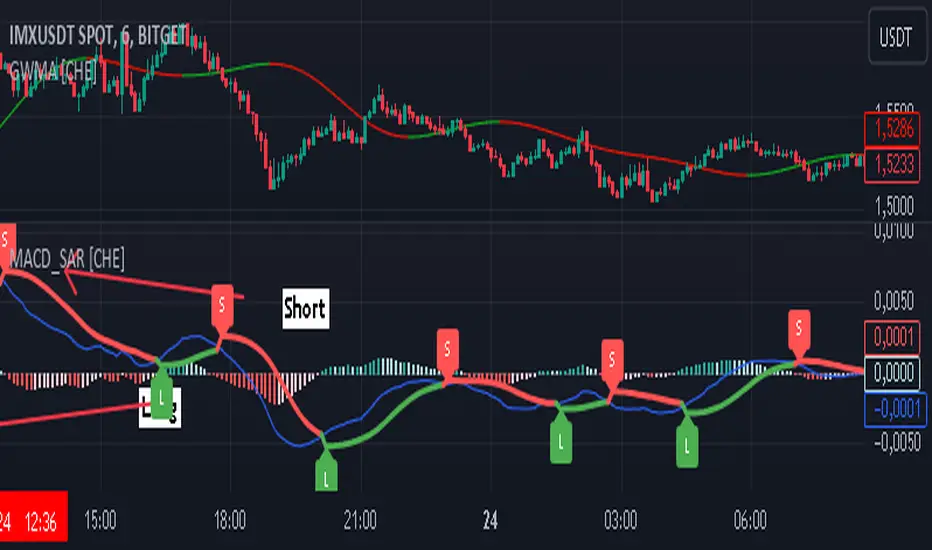
MACD with SAR Indicator [CHE] MACD with SAR Indicator
Introduction
"The whole is greater than the sum of its parts. " The "MACD with SAR Indicator" is an innovative technical analysis tool that combines the strengths of the Moving Average Convergence Divergence (MACD) indicator with the Parabolic Stop and Reverse (SAR) indicator. This indicator provides traders with an enhanced method to detect trend changes and determine optimal entry and exit points in the market by using the SAR based on the MACD line to better identify reversal points. The combination generates clear trend reversal signals, which are visually represented through long (L) and short (S) signals on the chart.
Originality and Usefulness
This indicator differs from traditional MACD or SAR indicators by combining the trend-following calculations of the SAR with the trend strength and momentum calculations of the MACD. This enables a more precise identification of trend changes and provides clear buy and sell signals, which is particularly useful for manual traders.
Key Features and Functionality
1. Combination of MACD and SAR
- Why this Combination?: The MACD is known for its ability to measure the strength and direction of a trend, while the SAR is specifically designed to identify reversal points. By combining these two indicators, traders can better understand both the trend strength and potential turning points in the market.
- How Components Work Together: The MACD measures the difference between fast and slow moving averages, indicating market momentum. The SAR follows the MACD line instead of the price and marks potential reversal points more accurately. When the MACD signals a new trend and the SAR confirms it, the indicator provides reliable trading opportunities.
2. Adjustable Parameters
- MACD Settings: Users can adjust the lengths of the fast and slow moving averages (default: 28 and 38 periods) and the signal smoothing (default: 9 periods) to tailor the indicator to different market conditions.
- SAR Settings: Users can adjust the start value (default: 0.01), increment (default: 0.01), and maximum value (default: 0.18) of the SAR to control sensitivity and responsiveness.
3. Visual Representation and Signals
- Color-Coded Histograms: The histogram shows the difference between the MACD and signal line and is color-coded to highlight the direction of the trend.
- Signal Labels: The indicator automatically adds "L" (Long) and "S" (Short) labels on the chart to show the current positions to traders.
4. Alert Settings
- Custom Alerts: Alerts can be set to notify traders when the MACD and SAR experience significant state changes, such as when the histogram switches from rising to falling or vice versa.
5. Toggle Display
- Display Mode: Users can toggle the display of the MACD_SAR oscillator and MACD to focus on the information most relevant to their trading strategy.
Application and Benefits
- Versatility: This indicator can be used in various market conditions and for different trading strategies, including trend following and reversal trading.
- Ease of Interpretation: The clear visual representation and automatic signals make it easier for traders to identify trading opportunities and track trends.
- Customizability: With numerous settings options, the indicator can be tailored to individual preferences and specific market conditions.
Conclusion
The "MACD with SAR Indicator" is a valuable tool for traders seeking precise and reliable signals to identify market trends and make profitable trading decisions. With its extensive customization options, powerful features, and the ability to toggle displays, this indicator provides excellent support for technical analysis.
By emphasizing the synergy between the MACD and SAR indicators, highlighting the default settings, and clarifying that the SAR is based on the MACD line and generates clear trend reversal signals through long and short labels, this revised description should help users understand the functionalities and advantages of your indicator while meeting TradingView's publication requirements.
Best regards Chervolino
Money Flow Index Crossover IndicatorThe "Money Flow Index Crossover Indicator" is a specialized technical analysis tool designed to assist traders by providing a clear visualization of potential buy and sell signals based on the Money Flow Index (MFI) and its smoothed moving average (SMA). This indicator delineates overbought and oversold zones, offering valuable insights into market dynamics. It operates as an oscillator on a separate pane, helping traders identify bullish and bearish market conditions with greater precision. By incorporating k-Nearest Neighbor (KNN) machine learning techniques, this indicator enhances the reliability and accuracy of the signals provided.
Originality and Usefulness:
This script is not just a simple mashup of existing indicators but integrates multiple components to create a unique and comprehensive analysis tool. The combined information from the MFI, its smoothed moving average, and the KNN machine learning techniques influence the form and accuracy of the Money Flow Index Average line and the Smoothed Money Flow Index line giving a visually helpful representation of overbought and oversold conditions. These lines are displayed in an oscillator style crossover, allowing users to visualize potential buy and sell zones for setting up potential signals. The user can adjust various settings of these tools behind the code to fine-tune the behavior and sensitivity of these lines. This integration provides a more robust and insightful trading tool that can adapt to different market conditions and trading styles.
How It Works:
Inputs:
MFI Settings:
Show Signals: Allows users to toggle the display of MFI and SMA crossing signals, which are critical for identifying potential market reversals.
Plot Amount: Determines the number of plots in the heat map, ranging from 2 to 28, enabling customization based on user preference.
Source: Defines the data source for MFI calculations, typically set to OHLC4 for a balanced view of price movements.
Smooth Initial MFI Length: Specifies the smoothing length for the initial MFI calculations to reduce noise and enhance signal clarity.
MFI SMA Length: Sets the length for the SMA used to smooth the MFI average, providing a more stable reference line.
Machine Learning Settings:
Use KInSource: Option to average MFI data by adding a lookback to the source, improving the accuracy of historical comparisons.
KNN Distance Requirement: Defines the distance calculation method for KNN (Max, Min, Both) to refine the data filtering process.
Machine Learning Length: Specifies the amount of machine learning data stored for smoothing results, balancing between responsiveness and stability.
KNN Length: Sets the number of KNN used to calculate the allowable distance range, enhancing the precision of the machine learning model.
Fast and Slow Lengths: Defines the lengths for fast and slow MFI calculations, allowing the indicator to capture different market dynamics.
Smoothing Length: Determines the length at which MFI calculations start for a more smoothed result, reducing false signals.
Variables and Functions:
KNN Function: Filters machine learning data to calculate valid distances based on defined criteria, ensuring more accurate MFI averages.
MFI Calculations: Computes both fast and slow MFI values, applies smoothing, and stores them for KNN processing to refine signal generation.
MFI KNN Calculation: Uses the KNN function to calculate the machine learning average of MFI values, enhancing signal reliability.
MFI Average and SMA: Calculates the average and smoothed MFI values, which are crucial for determining crossover signals.
Calculations:
MFI Values: Calculates current fast and slow MFI values and applies smoothing to reduce market noise.
Storage Arrays: Stores MFI data in arrays for KNN processing, enabling historical comparison and pattern recognition.
KNN Processing: Computes the machine learning average of MFI values using the KNN function, improving the robustness of signals.
MFI Average: Scales the MFI average to fit the heat map and calculates the smoothed SMA, providing a clear visual representation of trends.
Crossover Signals: Identifies bullish (MFI crossing above SMA) and bearish (MFI crossing below SMA) signals, which are key for making trading decisions.
Plots and Visuals:
MFI Average and SMA Lines: Plots the MFI average and smoothed SMA on the chart, allowing traders to easily visualize market trends and potential reversals.
Zones: Defines and plots overbought, neutral, and oversold zones for easy visualization. The recommended settings for these zones are:
Overbought Zone: Level set to approximately 24.6, indicating a potential market top.
Neutral Zone: Level set to 14, representing a balanced market condition.
Oversold Zone: Level set to 5.4, signaling a potential market bottom.
Crossover Marks: Plots circles on the chart to indicate bullish and bearish crossover signals, making it easier to spot entry and exit points.
Visual Alerts:
Bullish and Bearish Alerts: one can see overbought and oversold conditions and up alert conditions for bullish and bearish MFI crossover signals, enabling traders to have access to visual cues when these events are on trajectory to occur and, if they occur, act promptly with the visual representation of its zones.
Why It's Helpful:
The "Money Flow Index Crossover Indicator" provides traders with a sophisticated tool to identify potential buy and sell conditions based on the combined information of the MFI and its smoothed moving average. The KNN machine learning techniques enhance the accuracy of this indicator's clear visual representation of overbought, neutral, and oversold zones. This combination of data represented on the chart helps traders make informed decisions about market conditions. This indicator is particularly useful for traders looking to refine their entry and exit points by leveraging advanced data analysis in respect to overbought and oversold conditions.
Disclaimer:
This indicator is intended to assist traders in making informed decisions based on technical analysis. However, it is not a guarantee of future performance and should be used in conjunction with other analysis techniques and risk management practices. Past performance is not indicative of future results, and traders should exercise caution and perform their own due diligence before making any trading decisions.

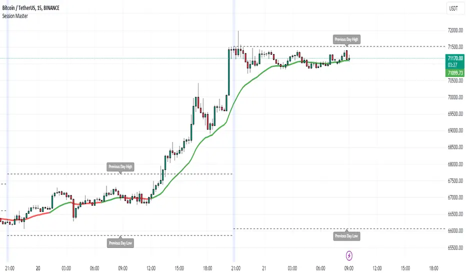
Session MasterSession Master Indicator
Overview
The "Session Master" indicator is a unique tool designed to enhance trading decisions by providing visual cues and relevant information during the critical last 15 minutes of a trading session. It also integrates advanced trend analysis using the Average Directional Index (ADX) and Directional Movement Index (DI) to offer insights into market trends and potential entry/exit points.
Originality and Functionality
This script combines session timing, visual alerts, and trend analysis in a cohesive manner to give traders a comprehensive view of market behavior as the trading day concludes. Here’s a breakdown of its key features:
Last 15 Minutes Highlight : The script identifies the last 15 minutes of the trading session and highlights this period with a semi-transparent blue background, helping traders focus on end-of-day price movements.
Previous Session High and Low : The script dynamically plots the high and low of the previous trading session. These levels are crucial for identifying support and resistance and are highlighted with dashed lines and labeled for easy identification during the last 15 minutes of the current session.
Directional Movement and Trend Analysis : Using a combination of ADX and DI, the script calculates and plots trend strength and direction. A 21-period Exponential Moving Average (EMA) is plotted with color coding (green for bullish and red for bearish) based on the DI difference, offering clear visual cues about the market trend.
Technical Explanation
Last 15 Minutes Highlight:
The script checks the current time and compares it to the session’s last 15 minutes.
If within this period, the background color is changed to a semi-transparent blue to alert the trader.
Previous Session High and Low:
The script retrieves the high and low of the previous daily session.
During the last 15 minutes of the session, these levels are plotted as dashed lines and labeled appropriately.
ADX and DI Calculation:
The script calculates the True Range, Directional Movement (both positive and negative), and smoothes these values over a specified length (28 periods by default).
It then computes the Directional Indicators (DI+ and DI-) and the ADX to gauge trend strength.
The 21-period EMA is plotted with dynamic color changes based on the DI difference to indicate trend direction.
How to Use
Highlight Key Moments: Use the blue background highlight to concentrate on market movements in the critical last 15 minutes of the trading session.
Identify Key Levels: Pay attention to the plotted high and low of the previous session as they often act as significant support and resistance levels.
Assess Trend Strength: Use the ADX and DI values to understand the strength and direction of the market trend, aiding in making informed trading decisions.
EMA for Entry/Exit: Use the color-coded 21-period EMA for potential entry and exit signals based on the trend direction indicated by the DI.
Conclusion
The "Session Master" indicator is a powerful tool designed to help traders make informed decisions during the crucial end-of-session period. By combining session timing, previous session levels, and advanced trend analysis, it provides a comprehensive overview that is both informative and actionable. This script is particularly useful for intraday traders looking to optimize their strategies around session close times.
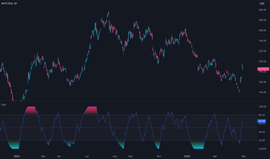
Slow Volume Strength Index (SVSI)The Slow Volume Strength Index (SVSI), introduced by Vitali Apirine in Stocks & Commodities (Volume 33, Chapter 6, Page 28-31), is a momentum oscillator inspired by the Relative Strength Index (RSI). It gauges buying and selling pressure by analyzing the disparity between average volume on up days and down days, relative to the underlying price trend. Positive volume signifies closes above the exponential moving average (EMA), while negative volume indicates closes below. Flat closes register zero volume. The SVSI then applies a smoothing technique to this data and transforms it into an oscillator with values ranging from 0 to 100.
Traders can leverage the SVSI in several ways:
1. Overbought/Oversold Levels: Standard thresholds of 80 and 20 define overbought and oversold zones, respectively.
2. Centerline Crossovers and Divergences: Signals can be generated by the indicator line crossing a midline or by divergences from price movements.
3. Confirmation for Slow RSI: The SVSI can be used to confirm signals generated by the Slow Relative Strength Index (SRSI), another oscillator developed by Apirine.
🔹 Algorithm
In the original article, the SVSI is calculated using the following formula:
SVSI = 100 - (100 / (1 + SVS))
where:
SVS = Average Positive Volume / Average Negative Volume
* Volume is considered positive when the closing price is higher than the six-day EMA.
* Volume is considered negative when the closing price is lower than the six-day EMA.
* Negative volume values are expressed as absolute values (positive).
* If the closing price equals the six-day EMA, volume is considered zero (no change).
* When calculating the average volume, the indicator utilizes Wilder's smoothing technique, as described in his book "New Concepts In Technical Trading Systems."
Note that this indicator, the formula has been simplified to be
SVSI = 100 * Average Positive Volume / (Average Positive Volume + Average Negative Volume)
This formula achieves the same result as the original article's proposal, but in a more concise way and without the need for special handling of division by zero
🔹 Parameters
The SVSI calculation offers configurable parameters that can be adjusted to suit individual trading styles and goals. While the default lookback periods are 6 for the EMA and 14 for volume smoothing, alternative values can be explored. Additionally, the standard overbought and oversold thresholds of 80 and 20 can be adapted to better align with the specific security being analyzed.
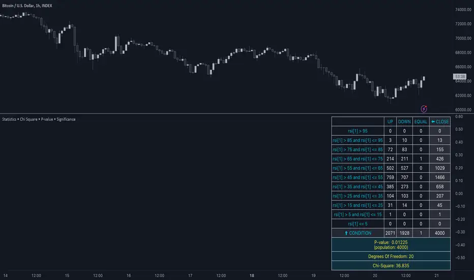
Statistics • Chi Square • P-value • SignificanceThe Statistics • Chi Square • P-value • Significance publication aims to provide a tool for combining different conditions and checking whether the outcome is significant using the Chi-Square Test and P-value.
🔶 USAGE
The basic principle is to compare two or more groups and check the results of a query test, such as asking men and women whether they want to see a romantic or non-romantic movie.
–––––––––––––––––––––––––––––––––––––––––––––
| | ROMANTIC | NON-ROMANTIC | ⬅︎ MOVIE |
–––––––––––––––––––––––––––––––––––––––––––––
| MEN | 2 | 8 | 10 |
–––––––––––––––––––––––––––––––––––––––––––––
| WOMEN | 7 | 3 | 10 |
–––––––––––––––––––––––––––––––––––––––––––––
|⬆︎ SEX | 10 | 10 | 20 |
–––––––––––––––––––––––––––––––––––––––––––––
We calculate the Chi-Square Formula, which is:
Χ² = Σ ( (Observed Value − Expected Value)² / Expected Value )
In this publication, this is:
chiSquare = 0.
for i = 0 to rows -1
for j = 0 to colums -1
observedValue = aBin.get(i).aFloat.get(j)
expectedValue = math.max(1e-12, aBin.get(i).aFloat.get(colums) * aBin.get(rows).aFloat.get(j) / sumT) //Division by 0 protection
chiSquare += math.pow(observedValue - expectedValue, 2) / expectedValue
Together with the 'Degree of Freedom', which is (rows − 1) × (columns − 1) , the P-value can be calculated.
In this case it is P-value: 0.02462
A P-value lower than 0.05 is considered to be significant. Statistically, women tend to choose a romantic movie more, while men prefer a non-romantic one.
Users have the option to choose a P-value, calculated from a standard table or through a math.ucla.edu - Javascript-based function (see references below).
Note that the population (10 men + 10 women = 20) is small, something to consider.
Either way, this principle is applied in the script, where conditions can be chosen like rsi, close, high, ...
🔹 CONDITION
Conditions are added to the left column ('CONDITION')
For example, previous rsi values (rsi ) between 0-100, divided in separate groups
🔹 CLOSE
Then, the movement of the last close is evaluated
UP when close is higher then previous close (close )
DOWN when close is lower then previous close
EQUAL when close is equal then previous close
It is also possible to use only 2 columns by adding EQUAL to UP or DOWN
UP
DOWN/EQUAL
or
UP/EQUAL
DOWN
In other words, when previous rsi value was between 80 and 90, this resulted in:
19 times a current close higher than previous close
14 times a current close lower than previous close
0 times a current close equal than previous close
However, the P-value tells us it is not statistical significant.
NOTE: Always keep in mind that past behaviour gives no certainty about future behaviour.
A vertical line is drawn at the beginning of the chosen population (max 4990)
Here, the results seem significant.
🔹 GROUPS
It is important to ensure that the groups are formed correctly. All possibilities should be present, and conditions should only be part of 1 group.
In the example above, the two top situations are acceptable; close against close can only be higher, lower or equal.
The two examples at the bottom, however, are very poorly constructed.
Several conditions can be placed in more than 1 group, and some conditions are not integrated into a group. Even if the results are significant, they are useless because of the group formation.
A population count is added as an aid to spot errors in group formation.
In this example, there is a discrepancy between the population and total count due to the absence of a condition.
The results when rsi was between 5-25 are not included, resulting in unreliable results.
🔹 PRACTICAL EXAMPLES
In this example, we have specific groups where the condition only applies to that group.
For example, the condition rsi > 55 and rsi <= 65 isn't true in another group.
Also, every possible rsi value (0 - 100) is present in 1 of the groups.
rsi > 15 and rsi <= 25 28 times UP, 19 times DOWN and 2 times EQUAL. P-value: 0.01171
When looking in detail and examining the area 15-25 RSI, we see this:
The population is now not representative (only checking for RSI between 15-25; all other RSI values are not included), so we can ignore the P-value in this case. It is merely to check in detail. In this case, the RSI values 23 and 24 seem promising.
NOTE: We should check what the close price did without any condition.
If, for example, the close price had risen 100 times out of 100, this would make things very relative.
In this case (at least two conditions need to be present), we set 1 condition at 'always true' and another at 'always false' so we'll get only the close values without any condition:
Changing the population or the conditions will change the P-value.
In the following example, the outcome is evaluated when:
close value from 1 bar back is higher than the close value from 2 bars back
close value from 1 bar back is lower/equal than the close value from 2 bars back
Or:
close value from 1 bar back is higher than the close value from 2 bars back
close value from 1 bar back is equal than the close value from 2 bars back
close value from 1 bar back is lower than the close value from 2 bars back
In both examples, all possibilities of close against close are included in the calculations. close can only by higher, equal or lower than close
Both examples have the results without a condition included (5 = 5 and 5 < 5) so one can compare the direction of current close.
🔶 NOTES
• Always keep in mind that:
Past behaviour gives no certainty about future behaviour.
Everything depends on time, cycles, events, fundamentals, technicals, ...
• This test only works for categorical data (data in categories), such as Gender {Men, Women} or color {Red, Yellow, Green, Blue} etc., but not numerical data such as height or weight. One might argue that such tests shouldn't use rsi, close, ... values.
• Consider what you're measuring
For example rsi of the current bar will always lead to a close higher than the previous close, since this is inherent to the rsi calculations.
• Be careful; often, there are na -values at the beginning of the series, which are not included in the calculations!
• Always keep in mind considering what the close price did without any condition
• The numbers must be large enough. Each entry must be five or more. In other words, it is vital to make the 'population' large enough.
• The code can be developed further, for example, by splitting UP, DOWN in close UP 1-2%, close UP 2-3%, close UP 3-4%, ...
• rsi can be supplemented with stochRSI, MFI, sma, ema, ...
🔶 SETTINGS
🔹 Population
• Choose the population size; in other words, how many bars you want to go back to. If fewer bars are available than set, this will be automatically adjusted.
🔹 Inputs
At least two conditions need to be chosen.
• Users can add up to 11 conditions, where each condition can contain two different conditions.
🔹 RSI
• Length
🔹 Levels
• Set the used levels as desired.
🔹 Levels
• P-value: P-value retrieved using a standard table method or a function.
• Used function, derived from Chi-Square Distribution Function; JavaScript
LogGamma(Z) =>
S = 1
+ 76.18009173 / Z
- 86.50532033 / (Z+1)
+ 24.01409822 / (Z+2)
- 1.231739516 / (Z+3)
+ 0.00120858003 / (Z+4)
- 0.00000536382 / (Z+5)
(Z-.5) * math.log(Z+4.5) - (Z+4.5) + math.log(S * 2.50662827465)
Gcf(float X, A) => // Good for X > A +1
A0=0., B0=1., A1=1., B1=X, AOLD=0., N=0
while (math.abs((A1-AOLD)/A1) > .00001)
AOLD := A1
N += 1
A0 := A1+(N-A)*A0
B0 := B1+(N-A)*B0
A1 := X*A0+N*A1
B1 := X*B0+N*B1
A0 := A0/B1
B0 := B0/B1
A1 := A1/B1
B1 := 1
Prob = math.exp(A * math.log(X) - X - LogGamma(A)) * A1
1 - Prob
Gser(X, A) => // Good for X < A +1
T9 = 1. / A
G = T9
I = 1
while (T9 > G* 0.00001)
T9 := T9 * X / (A + I)
G := G + T9
I += 1
G *= math.exp(A * math.log(X) - X - LogGamma(A))
Gammacdf(x, a) =>
GI = 0.
if (x<=0)
GI := 0
else if (x
Chisqcdf = Gammacdf(Z/2, DF/2)
Chisqcdf := math.round(Chisqcdf * 100000) / 100000
pValue = 1 - Chisqcdf
🔶 REFERENCES
mathsisfun.com, Chi-Square Test
Chi-Square Distribution Function
BAERMThe Bitcoin Auto-correlation Exchange Rate Model: A Novel Two Step Approach
THIS IS NOT FINANCIAL ADVICE. THIS ARTICLE IS FOR EDUCATIONAL AND ENTERTAINMENT PURPOSES ONLY.
If you enjoy this software and information, please consider contributing to my lightning address
Prelude
It has been previously established that the Bitcoin daily USD exchange rate series is extremely auto-correlated
In this article, we will utilise this fact to build a model for Bitcoin/USD exchange rate. But not a model for predicting the exchange rate, but rather a model to understand the fundamental reasons for the Bitcoin to have this exchange rate to begin with.
This is a model of sound money, scarcity and subjective value.
Introduction
Bitcoin, a decentralised peer to peer digital value exchange network, has experienced significant exchange rate fluctuations since its inception in 2009. In this article, we explore a two-step model that reasonably accurately captures both the fundamental drivers of Bitcoin’s value and the cyclical patterns of bull and bear markets. This model, whilst it can produce forecasts, is meant more of a way of understanding past exchange rate changes and understanding the fundamental values driving the ever increasing exchange rate. The forecasts from the model are to be considered inconclusive and speculative only.
Data preparation
To develop the BAERM, we used historical Bitcoin data from Coin Metrics, a leading provider of Bitcoin market data. The dataset includes daily USD exchange rates, block counts, and other relevant information. We pre-processed the data by performing the following steps:
Fixing date formats and setting the dataset’s time index
Generating cumulative sums for blocks and halving periods
Calculating daily rewards and total supply
Computing the log-transformed price
Step 1: Building the Base Model
To build the base model, we analysed data from the first two epochs (time periods between Bitcoin mining reward halvings) and regressed the logarithm of Bitcoin’s exchange rate on the mining reward and epoch. This base model captures the fundamental relationship between Bitcoin’s exchange rate, mining reward, and halving epoch.
where Yt represents the exchange rate at day t, Epochk is the kth epoch (for that t), and epsilont is the error term. The coefficients beta0, beta1, and beta2 are estimated using ordinary least squares regression.
Base Model Regression
We use ordinary least squares regression to estimate the coefficients for the betas in figure 2. In order to reduce the possibility of over-fitting and ensure there is sufficient out of sample for testing accuracy, the base model is only trained on the first two epochs. You will notice in the code we calculate the beta2 variable prior and call it “phaseplus”.
The code below shows the regression for the base model coefficients:
\# Run the regression
mask = df\ < 2 # we only want to use Epoch's 0 and 1 to estimate the coefficients for the base model
reg\_X = df.loc\ [mask, \ \].shift(1).iloc\
reg\_y = df.loc\ .iloc\
reg\_X = sm.add\_constant(reg\_X)
ols = sm.OLS(reg\_y, reg\_X).fit()
coefs = ols.params.values
print(coefs)
The result of this regression gives us the coefficients for the betas of the base model:
\
or in more human readable form: 0.029, 0.996869586, -0.00043. NB that for the auto-correlation/momentum beta, we did NOT round the significant figures at all. Since the momentum is so important in this model, we must use all available significant figures.
Fundamental Insights from the Base Model
Momentum effect: The term 0.997 Y suggests that the exchange rate of Bitcoin on a given day (Yi) is heavily influenced by the exchange rate on the previous day. This indicates a momentum effect, where the price of Bitcoin tends to follow its recent trend.
Momentum effect is a phenomenon observed in various financial markets, including stocks and other commodities. It implies that an asset’s price is more likely to continue moving in its current direction, either upwards or downwards, over the short term.
The momentum effect can be driven by several factors:
Behavioural biases: Investors may exhibit herding behaviour or be subject to cognitive biases such as confirmation bias, which could lead them to buy or sell assets based on recent trends, reinforcing the momentum.
Positive feedback loops: As more investors notice a trend and act on it, the trend may gain even more traction, leading to a self-reinforcing positive feedback loop. This can cause prices to continue moving in the same direction, further amplifying the momentum effect.
Technical analysis: Many traders use technical analysis to make investment decisions, which often involves studying historical exchange rate trends and chart patterns to predict future exchange rate movements. When a large number of traders follow similar strategies, their collective actions can create and reinforce exchange rate momentum.
Impact of halving events: In the Bitcoin network, new bitcoins are created as a reward to miners for validating transactions and adding new blocks to the blockchain. This reward is called the block reward, and it is halved approximately every four years, or every 210,000 blocks. This event is known as a halving.
The primary purpose of halving events is to control the supply of new bitcoins entering the market, ultimately leading to a capped supply of 21 million bitcoins. As the block reward decreases, the rate at which new bitcoins are created slows down, and this can have significant implications for the price of Bitcoin.
The term -0.0004*(50/(2^epochk) — (epochk+1)²) accounts for the impact of the halving events on the Bitcoin exchange rate. The model seems to suggest that the exchange rate of Bitcoin is influenced by a function of the number of halving events that have occurred.
Exponential decay and the decreasing impact of the halvings: The first part of this term, 50/(2^epochk), indicates that the impact of each subsequent halving event decays exponentially, implying that the influence of halving events on the Bitcoin exchange rate diminishes over time. This might be due to the decreasing marginal effect of each halving event on the overall Bitcoin supply as the block reward gets smaller and smaller.
This is antithetical to the wrong and popular stock to flow model, which suggests the opposite. Given the accuracy of the BAERM, this is yet another reason to question the S2F model, from a fundamental perspective.
The second part of the term, (epochk+1)², introduces a non-linear relationship between the halving events and the exchange rate. This non-linear aspect could reflect that the impact of halving events is not constant over time and may be influenced by various factors such as market dynamics, speculation, and changing market conditions.
The combination of these two terms is expressed by the graph of the model line (see figure 3), where it can be seen the step from each halving is decaying, and the step up from each halving event is given by a parabolic curve.
NB - The base model has been trained on the first two halving epochs and then seeded (i.e. the first lag point) with the oldest data available.
Constant term: The constant term 0.03 in the equation represents an inherent baseline level of growth in the Bitcoin exchange rate.
In any linear or linear-like model, the constant term, also known as the intercept or bias, represents the value of the dependent variable (in this case, the log-scaled Bitcoin USD exchange rate) when all the independent variables are set to zero.
The constant term indicates that even without considering the effects of the previous day’s exchange rate or halving events, there is a baseline growth in the exchange rate of Bitcoin. This baseline growth could be due to factors such as the network’s overall growth or increasing adoption, or changes in the market structure (more exchanges, changes to the regulatory environment, improved liquidity, more fiat on-ramps etc).
Base Model Regression Diagnostics
Below is a summary of the model generated by the OLS function
OLS Regression Results
\==============================================================================
Dep. Variable: logprice R-squared: 0.999
Model: OLS Adj. R-squared: 0.999
Method: Least Squares F-statistic: 2.041e+06
Date: Fri, 28 Apr 2023 Prob (F-statistic): 0.00
Time: 11:06:58 Log-Likelihood: 3001.6
No. Observations: 2182 AIC: -5997.
Df Residuals: 2179 BIC: -5980.
Df Model: 2
Covariance Type: nonrobust
\==============================================================================
coef std err t P>|t| \
\------------------------------------------------------------------------------
const 0.0292 0.009 3.081 0.002 0.011 0.048
logprice 0.9969 0.001 1012.724 0.000 0.995 0.999
phaseplus -0.0004 0.000 -2.239 0.025 -0.001 -5.3e-05
\==============================================================================
Omnibus: 674.771 Durbin-Watson: 1.901
Prob(Omnibus): 0.000 Jarque-Bera (JB): 24937.353
Skew: -0.765 Prob(JB): 0.00
Kurtosis: 19.491 Cond. No. 255.
\==============================================================================
Below we see some regression diagnostics along with the regression itself.
Diagnostics: We can see that the residuals are looking a little skewed and there is some heteroskedasticity within the residuals. The coefficient of determination, or r2 is very high, but that is to be expected given the momentum term. A better r2 is manually calculated by the sum square of the difference of the model to the untrained data. This can be achieved by the following code:
\# Calculate the out-of-sample R-squared
oos\_mask = df\ >= 2
oos\_actual = df.loc\
oos\_predicted = df.loc\
residuals\_oos = oos\_actual - oos\_predicted
SSR = np.sum(residuals\_oos \*\* 2)
SST = np.sum((oos\_actual - oos\_actual.mean()) \*\* 2)
R2\_oos = 1 - SSR/SST
print("Out-of-sample R-squared:", R2\_oos)
The result is: 0.84, which indicates a very close fit to the out of sample data for the base model, which goes some way to proving our fundamental assumption around subjective value and sound money to be accurate.
Step 2: Adding the Damping Function
Next, we incorporated a damping function to capture the cyclical nature of bull and bear markets. The optimal parameters for the damping function were determined by regressing on the residuals from the base model. The damping function enhances the model’s ability to identify and predict bull and bear cycles in the Bitcoin market. The addition of the damping function to the base model is expressed as the full model equation.
This brings me to the question — why? Why add the damping function to the base model, which is arguably already performing extremely well out of sample and providing valuable insights into the exchange rate movements of Bitcoin.
Fundamental reasoning behind the addition of a damping function:
Subjective Theory of Value: The cyclical component of the damping function, represented by the cosine function, can be thought of as capturing the periodic fluctuations in market sentiment. These fluctuations may arise from various factors, such as changes in investor risk appetite, macroeconomic conditions, or technological advancements. Mathematically, the cyclical component represents the frequency of these fluctuations, while the phase shift (α and β) allows for adjustments in the alignment of these cycles with historical data. This flexibility enables the damping function to account for the heterogeneity in market participants’ preferences and expectations, which is a key aspect of the subjective theory of value.
Time Preference and Market Cycles: The exponential decay component of the damping function, represented by the term e^(-0.0004t), can be linked to the concept of time preference and its impact on market dynamics. In financial markets, the discounting of future cash flows is a common practice, reflecting the time value of money and the inherent uncertainty of future events. The exponential decay in the damping function serves a similar purpose, diminishing the influence of past market cycles as time progresses. This decay term introduces a time-dependent weight to the cyclical component, capturing the dynamic nature of the Bitcoin market and the changing relevance of past events.
Interactions between Cyclical and Exponential Decay Components: The interplay between the cyclical and exponential decay components in the damping function captures the complex dynamics of the Bitcoin market. The damping function effectively models the attenuation of past cycles while also accounting for their periodic nature. This allows the model to adapt to changing market conditions and to provide accurate predictions even in the face of significant volatility or structural shifts.
Now we have the fundamental reasoning for the addition of the function, we can explore the actual implementation and look to other analogies for guidance —
Financial and physical analogies to the damping function:
Mathematical Aspects: The exponential decay component, e^(-0.0004t), attenuates the amplitude of the cyclical component over time. This attenuation factor is crucial in modelling the diminishing influence of past market cycles. The cyclical component, represented by the cosine function, accounts for the periodic nature of market cycles, with α determining the frequency of these cycles and β representing the phase shift. The constant term (+3) ensures that the function remains positive, which is important for practical applications, as the damping function is added to the rest of the model to obtain the final predictions.
Analogies to Existing Damping Functions: The damping function in the BAERM is similar to damped harmonic oscillators found in physics. In a damped harmonic oscillator, an object in motion experiences a restoring force proportional to its displacement from equilibrium and a damping force proportional to its velocity. The equation of motion for a damped harmonic oscillator is:
x’’(t) + 2γx’(t) + ω₀²x(t) = 0
where x(t) is the displacement, ω₀ is the natural frequency, and γ is the damping coefficient. The damping function in the BAERM shares similarities with the solution to this equation, which is typically a product of an exponential decay term and a sinusoidal term. The exponential decay term in the BAERM captures the attenuation of past market cycles, while the cosine term represents the periodic nature of these cycles.
Comparisons with Financial Models: In finance, damped oscillatory models have been applied to model interest rates, stock prices, and exchange rates. The famous Black-Scholes option pricing model, for instance, assumes that stock prices follow a geometric Brownian motion, which can exhibit oscillatory behavior under certain conditions. In fixed income markets, the Cox-Ingersoll-Ross (CIR) model for interest rates also incorporates mean reversion and stochastic volatility, leading to damped oscillatory dynamics.
By drawing on these analogies, we can better understand the technical aspects of the damping function in the BAERM and appreciate its effectiveness in modelling the complex dynamics of the Bitcoin market. The damping function captures both the periodic nature of market cycles and the attenuation of past events’ influence.
Conclusion
In this article, we explored the Bitcoin Auto-correlation Exchange Rate Model (BAERM), a novel 2-step linear regression model for understanding the Bitcoin USD exchange rate. We discussed the model’s components, their interpretations, and the fundamental insights they provide about Bitcoin exchange rate dynamics.
The BAERM’s ability to capture the fundamental properties of Bitcoin is particularly interesting. The framework underlying the model emphasises the importance of individuals’ subjective valuations and preferences in determining prices. The momentum term, which accounts for auto-correlation, is a testament to this idea, as it shows that historical price trends influence market participants’ expectations and valuations. This observation is consistent with the notion that the price of Bitcoin is determined by individuals’ preferences based on past information.
Furthermore, the BAERM incorporates the impact of Bitcoin’s supply dynamics on its price through the halving epoch terms. By acknowledging the significance of supply-side factors, the model reflects the principles of sound money. A limited supply of money, such as that of Bitcoin, maintains its value and purchasing power over time. The halving events, which reduce the block reward, play a crucial role in making Bitcoin increasingly scarce, thus reinforcing its attractiveness as a store of value and a medium of exchange.
The constant term in the model serves as the baseline for the model’s predictions and can be interpreted as an inherent value attributed to Bitcoin. This value emphasizes the significance of the underlying technology, network effects, and Bitcoin’s role as a medium of exchange, store of value, and unit of account. These aspects are all essential for a sound form of money, and the model’s ability to account for them further showcases its strength in capturing the fundamental properties of Bitcoin.
The BAERM offers a potential robust and well-founded methodology for understanding the Bitcoin USD exchange rate, taking into account the key factors that drive it from both supply and demand perspectives.
In conclusion, the Bitcoin Auto-correlation Exchange Rate Model provides a comprehensive fundamentally grounded and hopefully useful framework for understanding the Bitcoin USD exchange rate.

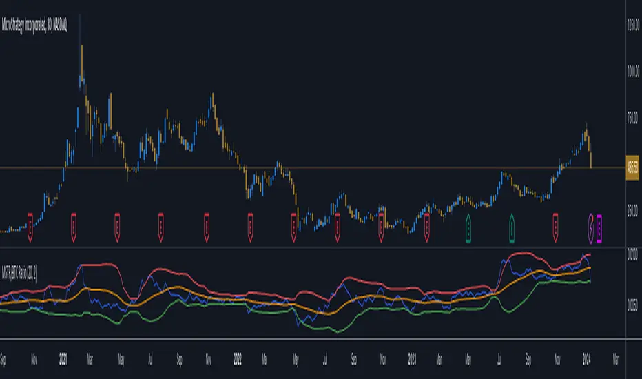
MicroStrategy / Bitcoin Market Cap RatioThis indicator offers a unique analytical perspective by comparing the market capitalization of MicroStrategy (MSTR) with that of Bitcoin (BTC) . Designed for investors and analysts interested in the correlation between MicroStrategy's financial performance and the Bitcoin market, the script calculates and visualizes the ratio of MSTR's market capitalization to Bitcoin's market capitalization.
Key Features:
Start Date: The script considers data starting from July 28, 2020, aligning with MicroStrategy's initial announcement to invest in Bitcoin.
Data Sources: It retrieves real-time data for MSTR's total shares outstanding, MSTR's stock price, and BTC's market capitalization.
Market Cap Calculations: The script calculates MicroStrategy's market cap by multiplying its stock price with the total shares outstanding. It then forms a ratio of MSTR's market cap to BTC's market cap.
Bollinger Bands: To add a layer of analysis, the script includes Bollinger Bands around the ratio, with customizable parameters for length and multiplier. These bands can help identify overbought or oversold conditions in the relationship between MSTR's and BTC's market values.
The indicator plots the MSTR/BTC market cap ratio and the Bollinger Bands, providing a clear visual representation of the relationship between these two market values over time.
This indicator is ideal for users who are tracking the impact of Bitcoin's market movements on MicroStrategy's valuation or vice versa. It provides a novel way to visualize and analyze the interconnectedness of a leading cryptocurrency asset and a major corporate investor in the space.
Elliott's Quadratic Momentum - Strategy [presentTrading]█ Introduction and How It Is Different
The "Elliott's Quadratic Momentum - Strategy" is a unique and innovative approach in the realm of technical trading. This strategy is a fusion of multiple SuperTrend indicators combined with an Elliott Wave-like pattern analysis, offering a comprehensive and dynamic trading tool. It stands apart from conventional strategies by incorporating multiple layers of trend analysis, thereby providing a more robust and nuanced view of market movements.
*Although the script doesn't explicitly analyze Elliott Wave patterns, it employs a wave-like approach by considering multiple SuperTrend indicators. Elliott Wave theory is based on the premise that markets move in predictable wave patterns. While this script doesn't identify specific Elliott Wave structures like impulsive and corrective waves, the sequential checking of trend conditions across multiple SuperTrend indicators mimics a wave-like progression.
BTC 8hr Long/Short Performance
Local Detail
█ Strategy, How It Works: Detailed Explanation
The core of this strategy lies in its multi-tiered approach:
1. Multiple SuperTrend Indicators:
The strategy employs four different SuperTrend indicators, each with unique ATR lengths and multipliers. These indicators offer various perspectives on market trends, ranging from short to long-term views.
By analyzing the convergence of these indicators, the strategy can pinpoint robust entry signals for both long and short positions.
2. Elliott Wave-like Pattern Recognition:
While not directly applying Elliott Wave theory, the strategy takes inspiration from its pattern recognition approach. It looks for alignments in market movements that resemble the characteristic waves of Elliott's theory.
This pattern recognition aids in confirming the signals provided by the SuperTrend indicators, adding an extra layer of validation to the trading signals.
3. Comprehensive Market Analysis:
By combining multiple indicators and pattern analysis, the strategy offers a holistic view of the market. This allows for capturing potential trend reversals and significant market moves early.
█ Trade Direction
The strategy is designed with flexibility in mind, allowing traders to select their preferred trading direction – Long, Short, or Both. This adaptability is key for traders looking to tailor their approach to different market conditions or personal trading styles. The strategy automatically adjusts its logic based on the chosen direction, ensuring that traders are always aligned with their strategic objectives.
█ Usage
To utilize the "Elliott's Quadratic Momentum - Strategy" effectively:
Traders should first determine their trading direction and adjust the SuperTrend settings according to their market analysis and risk appetite.
The strategy is versatile and can be applied across various time frames and asset classes, making it suitable for a wide range of trading scenarios.
It's particularly effective in trending markets, where the alignment of multiple SuperTrend indicators can provide strong trade signals.
█ Default Settings
Trading Direction: Configurable (Long, Short, Both)
SuperTrend Settings:
SuperTrend 1: ATR Length 7, Multiplier 4.0
SuperTrend 2: ATR Length 14, Multiplier 3.618
SuperTrend 3: ATR Length 21, Multiplier 3.5
SuperTrend 4: ATR Length 28, Multiplier 3.382
Additional Settings: Gradient effect for trend visualization, customizable color schemes for upward and downward trends.
7 consecutive closes above/below the 5-periodThis script looks for 7 consecutive closes above/below the 5-period SMA. The indicator is inspired by legendary trader Linda Raschke's work.
First are the two models for which the indicator was created, both inspired by Raschke:
1) Persistency of trend / Extended run setup.
Around 10-12 times per year we get a persistency of trend in instruments in general.
After 7 consecutive closes above/below the 5-period as price pulls back we can look to enter in the direction of the main trend as it moves up/down above/below 5 ma again. You should use price action trading to pinpoint the entries. Now try to hold this as long as possible. Way longer than you can percieve or think is possible. Up to 24-28 periods is what we are looking for in these cases.
2) Normal usage.
When the trend is not persistent, it is possible to use this as an oscillating signal, for a shorter term trade, where we can look for a short or long term reversal setup in price action.
3) I also use it at as a learning to see the swing trades clearer. You can also use it as a visual aid for developing new variances of the classic swing trading setup.
Read and listen to Linda Raschkes work to learn more.

7 Closes above/below 5 SMAThis script looks for 7 consecutive closes above/below the 5-period SMA. The indicator is inspired by legendary trader Linda Raschke's work.
Usage
The script can can be used in three main ways. I think you will find more uses.
First are the two models for which the indicator was created, both inspired by Raschke:
1) Persistency of trend / Extended run setup.
Around 10-12 times per year we get a persistency of trend in instruments in general.
After 7 consecutive closes above/below the 5-period as price pulls back we can look to enter in the direction of the main trend as it moves up/down above/below 5 ma again. You should use price action trading to pinpoint the entries. Now try to hold this as long as possible. Way longer than you can percieve or think is possible. Up to 24-28 periods is what we are looking for in these cases.
2) Normal usage.
When the trend is not persistent, it is possible to use this as an oscillating signal, for a shorter term trade, where we can look for a short or long term reversal setup in price action.
3) I also use it at as a learning to see the swing trades clearer. You can also use it as a visual aid for developing new variances of the classic swing trading setup.
Read and listen to Linda Raschkes work to learn more.
TIme frames
The principles works in all time frames but may change depending on calendar differences. We will see more instances/year in shorter time frames.
Why closes above the 5 SMA
As you may or may not know the 5 SMA is a very important indicator. You can think of it like this, If price is above 5, it is innocent until proven guilty but if price is below 5 we use the french law system which means it is guilty until proven innocent. 7 closes above 5 is a very good predictor of possible short term direction changes.
Use together with:
I prefer to use this indicator together with either regular SMA:s, one short and one macro term. For example 10 ma and 100 ma.
Or you can use it with a a Hull 21-period MA together with a 240-period WMA.
Settings:
I added settings so you can change preferences for changing shape, where to display the shape and in what color
Visual aid
I wanted to keep one dot for each consecutive day, this way we will get a grouping of days and dots. The amount in this group can be of use in itself to inform you of the strength of trend. This can inform you if this oscillation predicts a short term eversal or a continuation. You need skills in reading price action to use this to your advantage.

Pure Morning 2.0 - Candlestick Pattern Doji StrategyThe new "Pure Morning 2.0 - Candlestick Pattern Doji Strategy" is a trend-following, intraday cryptocurrency trading system authored by devil_machine.
The system identifies Doji and Morning Doji Star candlestick formations above the EMA60 as entry points for long trades.
For best results we recommend to use on 15-minute, 30-minute, or 1-hour timeframes, and are ideal for high-volatility markets.
The strategy also utilizes a profit target or trailing stop for exits, with stop loss set at the lowest low of the last 100 candles. The strategy's configuration details, such as Doji tolerance, and exit configurations are adjustable.
In this new version 2.0, we've incorporated a new selectable filter. Since the stop loss is set at the lowest low, this filter ensures that this value isn't too far from the entry price, thereby optimizing the Risk-Reward ratio.
In the specific case of ALPINE, a 9% Take-Profit and and Stop-Loss at Lowest Low of the last 100 candles were set, with an activated trailing-stop percentage, Max Loss Filter is not active.
Name : Pure Morning 2.0 - Candlestick Pattern Doji Strategy
Author : @devil_machine
Category : Trend Follower based on candlestick patterns.
Operating mode : Spot or Futures (only long).
Trades duration : Intraday
Timeframe : 15m, 30m, 1H
Market : Crypto
Suggested usage : Short-term trading, when the market is in trend and it is showing high volatility .
Entry : When a Doji or Morning Doji Star formation occurs above the EMA60.
Exit : Profit target or Trailing stop, Stop loss on the lowest low of the last 100 candles.
Configuration :
- Doji Settings (tolerances) for Entry Condition
- Max Loss Filter (Lowest Low filter)
- Exit Long configuration
- Trailing stop
Backtesting :
⁃ Exchange: BINANCE
⁃ Pair: ALPINEUSDT
⁃ Timeframe: 30m
⁃ Fee: 0.075%
⁃ Slippage: 1
- Initial Capital: 10000 USDT
- Position sizing: 10% of Equity
- Start: 2022-02-28 (Out Of Sample from 2022-12-23)
- Bar magnifier: on
Disclaimer : Risk Management is crucial, so adjust stop loss to your comfort level. A tight stop loss can help minimise potential losses. Use at your own risk.
How you or we can improve? Source code is open so share your ideas!
Leave a comment and smash the boost button!
Thanks for your attention, happy to support the TradingView community.

RSI, SRSI, MACD and DMI cross - Open source codeHello,
I'm a passionate trader who has spent years studying technical analysis and exploring different trading strategies. Through my research, I've come to realize that certain indicators are essential tools for conducting accurate market analysis and identifying profitable trading opportunities. In particular, I've found that the RSI, SRSI, MACD cross, and Di cross indicators are crucial for my trading success.
Detailed explanation:
The RSI is a momentum indicator that measures the strength of price movements. It is calculated by comparing the average of gains and losses over a certain period of time. In this indicator, the RSI is calculated based on the close price with a length of 14 periods.
The Stochastic RSI is a combination of the Stochastic Oscillator and the RSI. It is used to identify overbought and oversold conditions of the market. In this indicator, the Stochastic RSI is calculated based on the RSI with a length of 14 periods.
The MACD is a trend-following momentum indicator that shows the relationship between two moving averages of prices. It consists of two lines, the MACD line and the signal line, which are used to generate buy and sell signals. In this indicator, the MACD is calculated based on the close price with fast and slow lengths of 12 and 26 periods, respectively, and a signal length of 9 periods.
The DMI is a trend-following indicator that measures the strength of directional movement in the market. It consists of three lines, the Positive Directional Indicator (+DI), the Negative Directional Indicator (-DI), and the Average Directional Index (ADX), which are used to generate buy and sell signals. In this indicator, the DMI is calculated with a length of 14 periods and an ADX smoothing of 14 periods.
The indicator generates buy signals when certain conditions are met for each of these indicators.
1) For the RSI, a buy signal is generated when the RSI is below or equal to 35 and the Stochastic RSI %K is below or equal to 15, or when the RSI is below or equal to 28 the Stochastic RSI %K is below or equal to 15 or when the RSI is below or equal to 25 and the Stochastic RSI %K is below or equal to 10 or when the RSI is below or equal to 28.
2) For the MACD, a buy signal is generated when the MACD line is below 0, there is a change in the histogram from negative to positive, the MACD line and histogram are negative in the previous period, and the current histogram value is greater than 0.
3) For the DMI, a buy signal is generated when the Positive Directional Indicator (+DI) crosses above the Negative Directional Indicator (-DI), and the -DI is less than the +DI.
The indicator generates sell signals when certain conditions are met for each of these indicators:
1) For the RSI, a sell signal is generated when the RSI is above or equal to 75 and the Stochastic RSI %K is above or equal to 85, or when the RSI is above or equal to 80 and the Stochastic RSI %K is above or equal to 85, or when the RSI is above or equal to 85 and the Stochastic RSI %K is above or equal to 90 or when the RSI is above or equal to 82.
2)For the MACD, a sell signal is generated when the MACD line is above 0, there is a change in the histogram from positive to negative, the MACD line and histogram are positive in the previous period, and the current histogram value is less than the previous histogram value. On the other hand, a buy signal is generated when the MACD line is below 0, there is a change in the histogram from negative to positive, the MACD line and histogram are negative in the previous period, and the current histogram value is greater than the previous histogram value.
3)For the DMI a bearish signal is generated when plusDI crosses above minusDI, indicating that bulls are losing strength and bears are taking control.
The indicator uses a combination of these four indicators to generate potential buy and sell signals. The buy signals are generated when RSI and SRSI values are in oversold conditions, while sell signals are generated when RSI and SRSI values are in overbought conditions. The indicator also uses MACD crossovers and DMI crossovers to generate additional buy and sell signals.
When a signal is strong?
The use of multiple signals within a specific timeframe can increase the accuracy and reliability of the signals generated by this indicator. It is recommended to look for at least two signals within a range of 5-8 candles in order to increase the probability of a successful trade.
Why it's original?
1) There is no indicator in the library that combine all of these indicators and give you a 360 view
2)The combination of the RSI, Stochastic RSI, MACD, and DMI indicators in a single script it's unique and not available in the libray.
3)The specific parameters and conditions used to calculate the signals may be unique and not found in other scripts or libraries.
4)The use of plotshape() to plot the signals as shapes on the chart may be unique compared to other scripts that simply plot lines or bars to indicate signals.
5)The use of alertcondition() to trigger alerts based on the signals may be unique compared to other scripts that do not have custom alert functionality.
Keep attention!
It is important to note that no trading indicator or strategy is foolproof, and there is always a risk of losses in trading. While this indicator may provide useful information for making conclusions, it should not be used as the sole basis for making trading decisions. Traders should always use proper risk management techniques and consider multiple factors when making trading decisions.
Support me:)
If you find this new indicator helpful in your trading analysis, I would greatly appreciate your support! Please consider giving it a like, leaving feedback, or sharing it with your trading network. Your engagement will not only help me improve this tool but will also help other traders discover it and benefit from its features. Thank you for your support!
SPY 4 Hour Swing TraderThe purpose of this script is to spot 4 hour pivots that indicate ~30 trading day swings. As VIX starts to drop options trading will get more boring and as we get back on the bull and can benefit from swing trading strategy. Swing trading doesn't make a whole lot of sense when VIX is above 28. Seems to get best results on 4 hour chart for this one. This indicator spots a go long opportunity when the 5 ema crosses the 13 ema on the 4 hour along with the RSI > 50 and the ADX > 20 and Stoichastic values (smoothed line < 80 or line < 90) and close > last candle close and the True Range < 6. It also spots uses a couple different means to determine when to exit the trade. Sell condition is primarily when the 13 ema crosses the 5 ema and the MACD line crosses below the signal line and the smoothed Stoichastic appears oversold (greater than 60) and slop of RSI < -.2. Stop Losses and Take Profits are configurable in Inputs along with ability to include short trades plus other MACD and Stoichastic settings. If a stop loss is encountered the trade will close. Also once twice the expected move is encountered partial profits will taken and stop losses and take profits will be re-established based on most recent close. Also a VIX above 28 will trigger any open positions to close. If trying to use this for something other than SPXL it is best to update stop losses and take profit percentages and check backtest results to ensure proper levels have been selected and the script gives satisfactory results.

Fetch Buy And Hold StrategyThis script was created as an experiment using ChatGPT. I actually woudn't recommend using the ai program to help you with your Pinescripts, as it makes a fair amount of mistakes. It was a fun experiment however.
The script is a simple buy and hold tool. Here's what it does:
- Everytime the rsi enters below the set treshold, a counter increases.
- The second increase of the counter happens when the price goes above the treshold, and then dips below the treshold again.
- The program would fire off a buy signal when the counter hits the number 3.
- After the buy. the counter will reset.
Lets take a look at the following example where the rsi treshold is 30:
- So the rsi dips below 30 and the initial counter is set from 0 to 1.
- The price rises which brings the rsi back to 40.
- Then another dip happens and the rsi is now 25, increasing the counter from 1 two.
- Rsi now dips to 23 and nothing happens.
- Rsi goes back up to 31, and dips back to 28 which puts the counter at 3. A buy singal is now fired and the counter is set to 0.
Nonfarm [TjnTjn]This indicator will draw a line on your chart to show the Nonfarm announcement date and a line showing the Nonfarm announcement time for that day.
Because normally the Nonfarm announcement date is not simply the first Friday of the month. Because there are days Nonfarm days can be 8 or 9 or 10.
By checking the entire history of nonfarm announcements, I found some more rules such as if the first Friday of the month hits a holiday, the nonfarm day will be the friday of the following week. The previous months are 28, 29, or 30 days and if the first Friday of this month is on the 3, 2 or 1, the nonfarm day will be the friday of the following week.
Since this type of indicator is not available on the Tradingview library, I have put it up for everyone's convenience to backtest the price movement on nonfarm days to better support trading or simply to avoid trading at time of announed nonfarm.

libKageMiscLibrary "libKageMisc"
Kage's Miscelaneous library
print(_value)
Print a numerical value in a label at last historical bar.
Parameters:
_value : (float) The value to be printed.
Returns: Nothing.
barsBackToDate(_year, _month, _day)
Get the number of bars we have to go back to get data from a specific date.
Parameters:
_year : (int) Year of the specific date.
_month : (int) Month of the specific date. Optional. Default = 1.
_day : (int) Day of the specific date. Optional. Default = 1.
Returns: (int) Number of bars to go back until reach the specific date.
bodySize(_index)
Calculates the size of the bar's body.
Parameters:
_index : (simple int) The historical index of the bar. Optional. Default = 0.
Returns: (float) The size of the bar's body in price units.
shadowSize(_direction)
Size of the current bar shadow. Either "top" or "bottom".
Parameters:
_direction : (string) Direction of the desired shadow.
Returns: (float) The size of the chosen bar's shadow in price units.
shadowBodyRatio(_direction)
Proportion of current bar shadow to the bar size
Parameters:
_direction : (string) Direction of the desired shadow.
Returns: (float) Ratio of the shadow size per body size.
bodyCloseRatio(_index)
Proportion of chosen bar body size to the close price
Parameters:
_index : (simple int) The historical index of the bar. Optional. Default = 0.()
Returns: (float) Ratio of the body size per close price.
lastDayOfMonth(_month)
Returns the last day of a month.
Parameters:
_month : (int) Month number.
Returns: (int) The number (28, 30 or 31) of the last day of a given month.
nameOfMonth(_month)
Return the short name of a month.
Parameters:
_month : (int) Month number.
Returns: (string) The short name ("Jan", "Feb"...) of a given month.
pl(_initialValue, _finalValue)
Calculate Profit/Loss between two values.
Parameters:
_initialValue : (float) Initial value.
_finalValue : (float) Final value = Initial value + delta.
Returns: (float) Profit/Loss as a percentual change.
gma(_Type, _Source, _Length)
Generalist Moving Average (GMA).
Parameters:
_Type : (string) Type of average to be used. Either "EMA", "HMA", "RMA", "SMA", "SWMA", "WMA" or "VWMA".
_Source : (series float) Series of values to process.
_Length : (simple int) Number of bars (length).
Returns: (float) The value of the chosen moving average.
xFormat(_percentValue, _minXFactor)
Transform a percentual value in a X Factor value.
Parameters:
_percentValue : (float) Percentual value to be transformed.
_minXFactor : (float) Minimum X Factor to that the conversion occurs. Optional. Default = 10.
Returns: (string) A formated string.
isLong()
Check if the open trade direction is long.
Returns: (bool) True if the open position is long.
isShort()
Check if the open trade direction is short.
Returns: (bool) True if the open position is short.
lastPrice()
Returns the entry price of the last openned trade.
Returns: (float) The last entry price.
barsSinceLastEntry()
Returns the number of bars since last trade was oppened.
Returns: (series int)
getBotNameFrosty()
Return the name of the FrostyBot Bot.
Returns: (string) A string containing the name.
getBotNameZig()
Return the name of the FrostyBot Bot.
Returns: (string) A string containing the name.
getTicksValue(_currencyValue)
Converts currency value to ticks
Parameters:
_currencyValue : (float) Value to be converted.
Returns: (float) Value converted to minticks.
getSymbol(_botName, _botCustomSymbol)
Formats the symbol string to be used with a bot
Parameters:
_botName : (string) Bot name constant. Either BOT_NAME_FROSTY or BOT_NAME_ZIG. Optional. Default is empty string.
_botCustomSymbol : (string) Custom string. Optional. Default is empy string.
Returns: (string) A string containing the symbol for the bot. If all arguments are empty, the current symbol is returned in Binance format.
showProfitLossBoard()
Calculates and shows a board of Profit/Loss through the years.
Returns: Nothing.
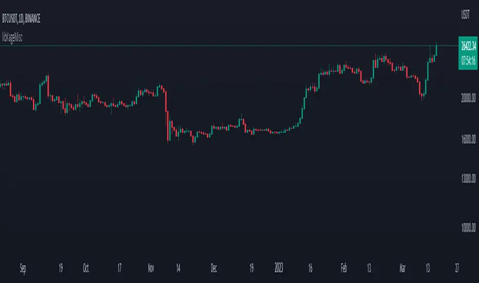
Forex Strength IndicatorThis indicator will display the strength of 8 currencies, EUR, AUD, NZD, JPY, USD, GBP, CHF, and CAD. Each line will represent each currency. Alongside that, Fibonacci levels will be plotted based on a standard deviation from linear regression, with customizable lengths.
For more steady Fibonacci levels, use higher lengths for both Standard Deviations and Linear Regression. All currency lines come from moving averages with options like EMA, SMA, WMA, RMA, HMA, SWMA, and Linear Regression.
When lines of the active pair are far from each other, it means higher divergence in those currency strengths among the other pairs. The closer the lines are, the lower the divergence.
You can use the Fibonacci levels as points for the reversal or end of the current trend. When the lines cross can be used as a parameter for a more accurate signal of the next movement.
All 28 pairs are loaded from the same time frame and will use the same moving average for all of them
Alerts from the line crossing are available.

Selected Dates Filter by @zeusbottradingWe are presenting you feature for strategies in Pine Script.
This function/pine script is about NOT opening trades on selected days. Real usage is for bank holidays or volatile days (PPI, CPI, Interest Rates etc.) in United States and United Kingdom from 2020 to 2030 (10 years of dates of bank holidays in mentioned countries above). Strategy is simple - SMA crossover of two lengts 14 and 28 with close source.
In pine script you can see we picked US and GB bank holidays. If you add this into your strategy, your bot will not open trades on those days. You must make it a rule or a condition. We use it as a rule in opening long/short trades.
You can also add some of your prefered dates, here is just example of our idea. If you want to add your preffered days you can find them on any site like forexfactory, myfxbook and so on. But don’t forget to add function “time_tradingday ! = YourChoosedDate” as it is writen lower in the pine script.
Sometimes the date is substituted for a different day, because the day of the holiday is on Saturday or Sunday.
Made with ❤️ for this community.
If you have any questions or suggestions, let us know.
The script is for informational and educational purposes only. Use of the script does not constitutes professional and/or financial advice. You alone the sole responsibility of evaluating the script output and risks associated with the use of the script. In exchange for using the script, you agree not to hold zeusbottrading TradingView user liable for any possible claim for damages arising from any decision you make based on use of the script.

TechnicalRating█ OVERVIEW
This library is a Pine Script™ programmer’s tool for incorporating TradingView's well-known technical ratings within their scripts. The ratings produced by this library are the same as those from the speedometers in the technical analysis summary and the "Rating" indicator in the Screener , which use the aggregate biases of 26 technical indicators to calculate their results.
█ CONCEPTS
Ensemble analysis
Ensemble analysis uses multiple weaker models to produce a potentially stronger one. A common form of ensemble analysis in technical analysis is the usage of aggregate indicators together in hopes of gaining further market insight and reinforcing trading decisions.
Technical ratings
Technical ratings provide a simplified way to analyze financial markets by combining signals from an ensemble of indicators into a singular value, allowing traders to assess market sentiment more quickly and conveniently than analyzing each constituent separately. By consolidating the signals from multiple indicators into a single rating, traders can more intuitively and easily interpret the "technical health" of the market.
Calculating the rating value
Using a variety of built-in TA functions and functions from our ta library, this script calculates technical ratings for moving averages, oscillators, and their overall result within the `calcRatingAll()` function.
The function uses the script's `calcRatingMA()` function to calculate the moving average technical rating from an ensemble of 15 moving averages and filters:
• Six Simple Moving Averages and six Exponential Moving Averages with periods of 10, 20, 30, 50, 100, and 200
• A Hull Moving Average with a period of 9
• A Volume-Weighted Moving Average with a period of 20
• An Ichimoku Cloud with a conversion line length of 9, base length of 26, and leading span B length of 52
The function uses the script's `calcRating()` function to calculate the oscillator technical rating from an ensemble of 11 oscillators:
• RSI with a period of 14
• Stochastic with a %K period of 14, a smoothing period of 3, and a %D period of 3
• CCI with a period of 20
• ADX with a DI length of 14 and an ADX smoothing period of 14
• Awesome Oscillator
• Momentum with a period of 10
• MACD with fast, slow, and signal periods of 12, 26, and 9
• Stochastic RSI with an RSI period of 14, a %K period of 14, a smoothing period of 3, and a %D period of 3
• Williams %R with a period of 14
• Bull Bear Power with a period of 50
• Ultimate Oscillator with fast, middle, and slow lengths of 7, 14, and 28
Each indicator is assigned a value of +1, 0, or -1, representing a bullish, neutral, or bearish rating. The moving average rating is the mean of all ratings that use the `calcRatingMA()` function, and the oscillator rating is the mean of all ratings that use the `calcRating()` function. The overall rating is the mean of the moving average and oscillator ratings, which ranges between +1 and -1. This overall rating, along with the separate MA and oscillator ratings, can be used to gain insight into the technical strength of the market. For a more detailed breakdown of the signals and conditions used to calculate the indicators' ratings, consult our Help Center explanation.
Determining rating status
The `ratingStatus()` function produces a string representing the status of a series of ratings. The `strongBound` and `weakBound` parameters, with respective default values of 0.5 and 0.1, define the bounds for "strong" and "weak" ratings.
The rating status is determined as follows:
Rating Value Rating Status
< -strongBound Strong Sell
< -weakBound Sell
-weakBound to weakBound Neutral
> weakBound Buy
> strongBound Strong Buy
By customizing the `strongBound` and `weakBound` values, traders can tailor the `ratingStatus()` function to fit their trading style or strategy, leading to a more personalized approach to evaluating ratings.
Look first. Then leap.
█ FUNCTIONS
This library contains the following functions:
calcRatingAll()
Calculates 3 ratings (ratings total, MA ratings, indicator ratings) using the aggregate biases of 26 different technical indicators.
Returns: A 3-element tuple: ( [(float) ratingTotal, (float) ratingOther, (float) ratingMA ].
countRising(plot)
Calculates the number of times the values in the given series increase in value up to a maximum count of 5.
Parameters:
plot : (series float) The series of values to check for rising values.
Returns: (int) The number of times the values in the series increased in value.
ratingStatus(ratingValue, strongBound, weakBound)
Determines the rating status of a given series based on its values and defined bounds.
Parameters:
ratingValue : (series float) The series of values to determine the rating status for.
strongBound : (series float) The upper bound for a "strong" rating.
weakBound : (series float) The upper bound for a "weak" rating.
Returns: (string) The rating status of the given series ("Strong Buy", "Buy", "Neutral", "Sell", or "Strong Sell").
Weird Renko StratThis strategy uses Renko, it generates a signal when there is a reversal in Renko. When using historical data, it provides a good entry and an okay exit. However, in a real-time environment, this strategy is subject to repaint and may produce a false signal.
As a result, the backtesting result should not be used as a metric to predict future results. It is highly recommended to forward-test the strategy before using it in real trading. I forward test it from 12/18/2022 to 12/21/2022 in paper trading, using the alert feature in Tradingview. I made 60 trades trading the BTCUSDT BINANCE 3 min with 26 as the param and under the condition that I use 20x margin, compounding my yield, and having 0 trading fee, a steady loss is generated: from $10 to $3.02.
This is quite interesting. As if I flip the signal from "Long" to "Short" and another way too, it will be a steady profit from $10 to $21.85. Hence, if I'm trying to anti-trade the real-time alert signal, the current "4 Days Result" will be good. Nevertheless, I still have to forward-test it for longer to see if it will fail eventually.
Dive into the setting of the strategy
- Margin is the leverage you use. 1 means 1x, 10 means 10x. It affects the backtest yield when you backtest
- Compound Yield button is for compound calculation, disable it to go back to normal backtesting
- Anti Strategy button is to do the opposite direction trade, when the original strat told you to "Long", you "Short" instead. Enable it to use the feature
- Param is the block size for the Renko chart
- Drawdown is just a visual tool for you in case you want to place a stop loss (represent by the semitransparent red area in the chart)
- From date Thru Date is to specify the backtest range of the strategy, This feature is turned off by default. It is controlled by the Max Backtest Timeframe which will be explain below
- Max Backtest Timeframe control the From date Thru Date function, disable it to enable the From Date Thru Date function
Param is the most important input in this strategy as it directly affects performance. It is highly recommended to backtest nearly all the possible parameters before deploying it in real trading. Some factors should be considered:
- Price of the asset (like an asset of 1 USD vs an asset of 10000 USD required different param)
- Timeframe (1-minute param is different than 1-month param)
I believe this is caused by the volatility of the selected timeframe since different timeframe has different volatility. Param should be fine-tuned before usage.
Here is the param I'm using:
BTCUSDT BINANCE 3min: 26
BTCUSDT BINANCE 5min: 28
BTCUSDT BINANCE 1day: 15
Background of the strategy:
- The strategy starts with $10 at the start of backtesting (customizable in setting)
- The trading fee is set to 0.00% which is not common for most of the popular exchanges (customizable in setting)
- The contract size is not a fixed amount, but it uses your balance to buy it at the open price. If you are using the compound mode, your balance will be your current total balance. If you are using the non-compound mode, it will just use the $10 you start with unless you change the amount you start with. If you are using a margin higher than 1, it will calculate the corresponding contract size properly based on your margin. (Only these options are allowed, you are not able to change them without changing the code)