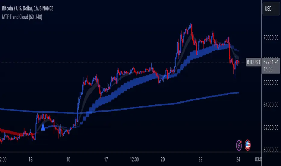
Multi-Timeframe Trend Cloud (EMA13/21) with Alerts Purpose:
This indicator combines trend analysis across multiple timeframes with alerts to help identify general trends and market shifts. It visualizes trends by creating EMA clouds (The area between EMA13 & EMA21), detects confirmed EMA crossovers, and can alert users when the price re-enters the cloud or interacts with the EMA200.
Input Parameters:
Lower Timeframe (LTF): Allows you to select the lower timeframe for trend analysis (e.g., 1 hour, 4 hours).
Higher Timeframe (HTF): Allows you to select the higher timeframe for the main trend reference (e.g., 4 hours, 1 day).
Fill Colors: You can customize the colors used to fill the areas between the EMA lines in both the higher and lower timeframes. Note: The LTF cloud defaults to transparent white so if you have a light background change the color in style settings.
The EMA's default to transparent but can be turned on in the style settings.
Calculating & Plotting EMAs:
The indicator calculates two Exponential Moving Averages (EMAs) on both the LTF and HTF: a faster 13-period EMA and a slower 21-period EMA.
Additionally, it calculates a 200-period EMA on the HTF.
These EMAs are plotted on your chart, providing a visual representation of the trend.
Identifying Trend States:
The script uses the relationships between the price and the 13-period and 21-period EMAs on the Higher Time Frame (HTF) to identify four distinct trend states, each depicted by a specific color to create the "Trend Cloud":
Strong Bull Trend: The 13-period EMA is above the 21-period EMA, and the price is above both EMAs. --- "Color 0" in HTF Trend style settings.
Broken Bullish Trend: The 13-period EMA is above the 21-period EMA but price has broken below both EMA's. --- "Color 3" in HTF Trend style settings.
Strong Bear Trend: The 13-period EMA is below the 21-period EMA, and the price is below both EMAs. --- "Color 2" in HTF Trend style settings.
Broken Bearish Trend: The 13-period EMA is below the 21-period EMA but price has broken above both EMA's. --- "Color 1" in HTF Trend style settings.
Important Note: The 200-period EMA is plotted for reference but is not directly used in determining the current trend state within this script.
Confirmed Crossover Signals:
The indicator plots upward or downward triangles to signal confirmed crossovers of the EMA13 and EMA21 on the HTF. A crossover is considered "confirmed" when it's followed by a candle closing on the same side of the crossing point, adding an extra layer of confidence to the signal.
Cloud Re-entry Alerts:
Receive alerts whenever the price re-enters the HTF cloud - aka "Trend".
EMA200 Retest Alerts:
Get alerts when the price touches the 200 EMA on the HTF. These alerts can be valuable for identifying potential trend reversals or trend continuation scenarios.
Benefits:
Clear Visual Representation: Easily visualize trends on both the lower and higher timeframes.
Confirmed Signals: Filter out false signals by focusing on confirmed crossovers.
Timely Alerts: Get instant notifications for important price actions, allowing you to react quickly to market opportunities.
Customizable: Tailor the indicator's appearance and alert settings to your preferences.
How to Use:
Add the indicator to your chart.
Select your desired LTF and HTF in the Inputs tab.
Customize the fill colors (and optional EMA line colors) in the Style tab.
Enable the alerts you want to receive in the Alerts tab.
Note: This indicator is a great tool for trend analysis, but it should be used with other forms of analysis and risk management techniques to make informed trading decisions.
在脚本中搜索"细算江西救护车家长倒赚了四万三+-医疗花费13万(家长视频)++医保报"
TrendMaster Pro IndicatorThe TrendMaster Pro Indicator is an advanced tool designed to assist traders in identifying potential buy and sell signals by leveraging a combination of exponential moving averages (EMAs), the relative strength index (RSI), and a custom volatility filter. This powerful indicator is suitable for traders of all levels and can be applied to various markets and timeframes, offering flexibility and reliability in trading decisions.
Key Features:
EMA Crossover Detection:
Utilizes a 5-period (short) and 13-period (long) EMA crossover to detect trend changes.
A bullish signal is generated when the 5 EMA crosses above the 13 EMA, indicating an upward trend.
A bearish signal is generated when the 5 EMA crosses below the 13 EMA, indicating a downward trend.
RSI Confirmation:
Incorporates a 14-period RSI to confirm the strength of detected trends.
A buy signal is validated when the RSI is above 50, indicating bullish momentum.
A sell signal is validated when the RSI is below 50, indicating bearish momentum.
Custom Volatility Filter:
Employs a volatility filter based on the standard deviation of closing prices over a specified period (default is 10 periods).
Ensures signals are only generated during periods of significant market movement, reducing noise and false signals.
The volatility threshold can be adjusted to suit different market conditions and trading styles.
How It Works:
EMA Crossover:
The TrendMaster Pro Indicator continuously monitors the crossover between the 5-period and 13-period EMAs.
A crossover event triggers the initial signal, suggesting a potential change in trend direction.
RSI Confirmation:
After an EMA crossover, the indicator checks the 14-period RSI value to confirm the trend's strength.
This confirmation step helps filter out weak or unreliable signals, ensuring only high-probability trades are considered.
Volatility Filter:
The indicator calculates the standard deviation of closing prices over the selected period to measure market volatility.
Signals are only generated if the volatility exceeds the user-defined threshold, ensuring that trades are made in active and dynamic market conditions.
How to Use:
Apply the Indicator:
Add the TrendMaster Pro Indicator to your trading chart via the TradingView platform.
Customize the EMA, RSI, and volatility settings according to your trading preferences and the specific market conditions.
Interpret Buy and Sell Signals:
Buy Signal: Look for a buy signal when the 5 EMA crosses above the 13 EMA, the RSI is above 50, and volatility exceeds the threshold. This combination indicates a strong bullish trend.
Sell Signal: Look for a sell signal when the 5 EMA crosses below the 13 EMA, the RSI is below 50, and volatility exceeds the threshold. This combination indicates a strong bearish trend.
Adjust Settings:
The default settings can be fine-tuned to match your trading strategy. Adjust the EMA lengths, RSI period, and volatility threshold to optimize the indicator for different assets and timeframes.
Unique Features:
Comprehensive Trend Detection: Combines multiple indicators (EMAs, RSI, volatility) to provide a holistic view of market trends.
Customizable: Easily adjustable settings allow traders to tailor the indicator to their specific needs and preferences.
Noise Reduction: The volatility filter ensures signals are generated only during significant market movements, improving signal accuracy and reliability.
Conclusion:
The TrendMaster Pro Indicator is a versatile and powerful tool that can enhance your trading strategy by providing clear and reliable buy and sell signals. Whether you are a day trader or a swing trader, this indicator can help you navigate the markets with confidence and precision. Add the TrendMaster Pro Indicator to your toolkit today and experience a new level of trading efficiency and effectiveness.

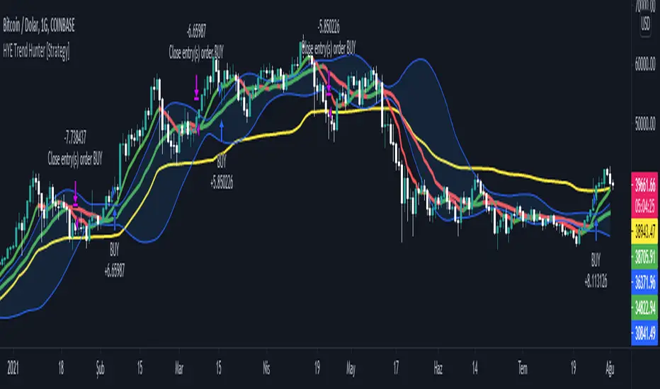
HYE Combo Market [Strategy] (Vwap Mean Reversion + Trend Hunter)In this strategy, I used a combination of trend hunter and vwap mean reversion strategies that I published before.
Trend Hunter Strategy:
Mean Reversion Vwap Strategy:
The results are quite impressive, especially for bitcoin.
While the hodl return for bitcoin was 13419%, the strategy's return in the same period was about 5 times (65000%) of this.
s3.tradingview.com
In this combo strategy, I made some changes to the original settings of the strategies used together and added some more new features.
Trend Hunter Strategy Settings: (Original / Combo)
- Slow Tenkansen Period : 9 / 9
- Slow Kijunsen Period : 26 / 13
- Fast Tenkansen Period : 5 / 3
- Fast Kijunsen Period : 13 / 7
- BB Length : 20 / 20
- BB Stdev : 2 / 2
- TSV Length : 13 / 20
- TSV Ema Length : 7 / 7
* I also added a "vidya moving average" to be used as a confirmation tool to open a long position. (Candle close must be above the vidya line.)
Vwap Mean Reversion Strategy Settings: (Original / Combo)
- Small Vwap : 2 / 8
- Big Vwap : 5 / 10
- Percent Below to Buy : 3 / 2
- RSI Period : 2 / 2
- RSI Ema Period : 5 / 5
- Maximum RSI Level for Buy : 30
* I also added a "mean vwap line" to be used for exits in this part of the strategy. In the original version, when small vwap crossovers big vwap, we close the position, but in this strategy we will wait for the close above the mean vwap.
TIPS AND WARNINGS
1-) The standard settings of this combo strategy is designed and tested with daily timeframe. For lower timeframes, you should change the strategy settings and find the best value for yourself.
2-) Only the mean vwap line is displayed on the graph. For a detailed view, you can delete the "//" marks from the plot codes in the strategy code.
3-) This is a strategy for educational and experimental purposes. It cannot be considered as investment advice. You should be careful and make your own risk assessment when opening real market trades using this strategy.
________________________________________________________
Bu stratejide, daha önce yayınladığım trend avcısı ve vwap ortalamaya geri dönüş stratejilerinin bir kombinasyonunu kullandım.
Sonuçlar özellikle bitcoin için oldukça etkileyici.
Bitcoin için hodl getirisi %13419 iken, stratejinin aynı dönemdeki getirisi bunun yaklaşık 5 katı (%65000) idi.
Bu kombo stratejide, birlikte kullanılan stratejilerin orijinal ayarlarında bazı değişiklikler yaptım ve bazı yeni özellikler ekledim.
Trend Avcısı Strateji Ayarları: (Orijinal / Combo)
- Yavaş Tenkansen Periyodu : 9 / 9
- Yavaş Kijunsen Periyodu : 26 / 13
- Hızlı Tenkansen Periyodu : 5 / 3
- Hızlı Kijunsen Periyodu : 13 / 7
- BB Uzunluğu : 20 / 20
- BB Standart Sapması : 2 / 2
- TSV Uzunluğu : 13 / 20
- TSV Ema Uzunluğu : 7 / 7
* Ayrıca long pozisyon açmak için onay aracı olarak kullanılmak üzere "vidya hareketli ortalama" ekledim. (Mum kapanışı vidya çizgisinin üzerinde olmalıdır.)
Vwap Ortalamaya Dönüş Stratejisi Ayarları: (Orijinal / Combo)
- Küçük Vwap : 2 / 8
- Büyük Vwap : 5 / 10
- Alış İçin Gerekli Fark Oranı : 3 / 2
- RSI Periyodu : 2 / 2
- RSI Ema Periyodu: 5 / 5
- Alış için gerekli maksimum RSI seviyesi : 30
* Stratejinin bu bölümünde pozisyondan çıkışlar için kullanılacak bir "ortalama vwap çizgisi" de ekledim. Orijinal versiyonda, küçük vwap, büyük vwap'ı yukarı kestiğinde pozisyonu kapatıyoruz, ancak bu stratejide, ortalama vwap'ın üzerindeki kapanışı bekleyeceğiz.
İPUÇLARI VE UYARILAR
1-) Bu birleşik stratejinin standart ayarları, günlük zaman dilimi ile tasarlanmış ve test edilmiştir. Daha düşük zaman dilimleri için strateji ayarlarını değiştirmeli ve kendiniz için en iyi değeri bulmalısınız.
2-) Grafikte sadece ortalama vwap çizgisi görüntülenir. Ayrıntılı bir görünüm için strateji kodundaki "plot" ile başlayan satırlarda grafikte görünmesini istediğiniz özelliğin önündeki "//" işaretlerini silebilirsiniz.
3-) Eğitim ve deneysel amaçlı bir stratejidir. Yatırım tavsiyesi olarak değerlendirilemez. Bu stratejiyi kullanarak gerçek piyasa işlem açarken dikkatli olmalı ve kendi risk değerlendirmenizi yapmalısınız.

HYE Trend Hunter [Strategy]*** Stratejinin Türkçe ve İngilizce açıklaması aşağıya eklenmiştir.
HYE Trend Hunter
In this strategy, two of the most basic data (price and volume) necessary for detecting trends as early as possible and entering the trade on time are used. In this context, the approaches of some classical and new generation indicators using price and volume have been taken into account.
The strategy is prepared to generate buy signals only. The following steps were followed to generate the buy and exit signals.
1-) First of all, the two most basic data of the strategy, “slow leading line” and “fast leading line” need to be calculated. For this, we use the formula of the “senkou span A” line of the indicator known as the Ichimoku Cloud. We also need to calculate lines known as tenkan sen and kijun sen in ichimoku because they are used in the calculation of this formula.
The high and low values of the candles are taken into account when calculating the Tenkansen, Kijunsen and Senkou Span A lines in the Ichimoku cloud. In this strategy, the highest and lowest values of the periodic VWAP are taken into account when calculating the "slow leading line" and "fast leading line". (The periodic vwap formula was coded and made available by @neolao on tradingviev). Also, in the ichimoku cloud, while the Senkou Span A line is plotted 26 periods into the future, we consider the values of the fast and slow leading lines in the last candle in this strategy.
ORIGINAL ICHIMOKU SPAN A FORMULA
Tenkansen = (Highest high of the last 9 candles + Lowest low of the last 9 candles) / 2
Kijunsen = (Highest high of the last 26 candles + Lowest low of the last 26 candles) / 2
Senkou Span A = Tenkansen + Kijunsen / 2
HYE TREND HUNTER SPAN A FORMULA*
Tenkansen = (Highest VWAP of the last 9 candles + Lowest VWAP of the last 9 candles) / 2
Kijunsen = (Highest VWAP of the last 26 candles + Lowest VWAP of the last 26 candles) / 2
Senkou Span A = Tenkansen + Kijunsen / 2
* We use the original ichimoku values 9 and 26 for the slow line, and 5 and 13 for the fast line. These settings can be changed from the strategy settings.
2-) At this stage, we have 2 lines that we obtained by using the formula of the ichimoku cloud, one of the most classical trend indicators, and by including the volume-weighted average price.
a-) Fast Leading Line (5-13)
b-) Slow Leading Line (9-26)
For the calculation we will do soon, we get a new value by taking the average of these two lines. Using this value, which is the average of the fast and slow leading lines, we plot the Bollinger Bands indicator, which is known as one of the most classic volatility indicators of technical analysis. Thus, we are trying to understand whether there is a volatility change in the market, which may mean the presence of a trend start. We will use this data in the calculation of buy-sell signals.
In the classical Bollinger Bands calculation, the standard deviation is calculated by applying a multiplier at the rate determined by the user (2 is used in the original settings) to the moving average calculated with the “closing price”, and this value is added or subtracted from the moving average and upper band and lower band lines are drawn.
In the HYE Trend Hunter Strategy, instead of the moving average calculated with the closing price in the Bollinger Band calculation, we consider the average of the fast and slow leading lines calculated in the 1st step and draw the Bollinger upper and lower bands accordingly. We use the values of 2 and 20 as the standard deviation and period, as in the original settings. These settings can also be changed from the strategy settings.
3-) At this stage, we have fast and slow leading lines trying to understand the trend direction using VWAP, and Bollinger lower and upper bands calculated by the average of these lines.
In this step, we will use another tool that will help us understand whether the invested market (forex, crypto, stocks) is gaining momentum in volume. The Time Segmented Volume indicator was created by the Worden Brothers Inc. and coded by @liw0 and @vitelot on tradingview. The TSV indicator segments the price and volume of an investment instrument according to certain time periods and makes calculations on comparing these price and volume data to reveal the buying and selling periods.
To trade in the buy direction on the HYE Trend Hunter Strategy, we look for the TSV indicator to be above 0 and above its exponential moving average value. TSV period and exponential moving average period settings (13 and 7) can also be changed in the strategy settings.
BUY SIGNAL
1-) Fast Leading Line value should be higher than the Fast Leading Line value in the previous candle.
2-) Slow Leading Line value should be higher than the Slow Leading Line value in the previous candle.
3-) Candle Closing value must be higher than the Upper Bollinger Band.
4-) TSV value must be greater than 0.
5-) TSV value must be greater than TSVEMA value.
EXIT SIGNAL
1-) Fast Leading Line value should be lower than the Fast Leading Line value in the previous candle.
2-) Slow Leading Line value should be lower than the Slow Leading Line value in the previous candle.
TIPS AND WARNINGS
1-) The standard settings of the strategy work better in higher timeframes (4-hour, daily, etc.). For lower timeframes, you should change the strategy settings and find the best value for yourself.
2-) All lines (fast and slow leading lines and Bollinger bands) except TSV are displayed on the strategy. For a simpler view, you can hide these lines in the strategy settings.
3-) You can see the color changes of the fast and slow leading lines as well as you can specify a single color for these lines in the strategy settings.
4-) It is an strategy for educational and experimental purposes. It cannot be considered as investment advice. You should be careful and make your own risk assessment when opening real market trades using this strategy.
_______________________________________________
HYE Trend Avcısı
Bu stratejide, trendlerin olabildiğince erken tespit edilebilmesi ve zamanında işleme girilebilmesi için gerekli olan en temel iki veriden (fiyat ve hacim) yararlanılmaktadır. Bu kapsamda, fiyat ve hacim kullanan bazı klasik ve yeni nesil indikatörlerin yaklaşımları dikkate alınmıştır.
Strateji yalnızca alış yönlü sinyaller üretecek şekilde hazırlanmıştır. Alış ve çıkış sinyallerinin üretilmesi için aşağıdaki adımlar izlenmiştir.
1-) Öncelikle, stratejinin en temel iki verisi olan “yavaş öncü çizgi” ve “hızlı öncü çizgi” hesaplamasının yapılması gerekiyor. Bunun için de Ichimoku Bulutu olarak bilinen indikatörün “senkou span A” çizgisinin formülünü kullanıyoruz. Bu formülün hesaplamasında kullanılmaları nedeniyle ichimoku’da tenkan sen ve kijun sen olarak bilinen çizgileri de hesaplamamız gerekiyor.
Ichimoku bulutunda Tenkansen, Kijunsen ve Senkou Span A çizgileri hesaplanırken mumların yüksek ve düşük değerleri dikkate alınıyor. Bu stratejide ise “yavaş öncü çizgi” ve “hızlı öncü çizgi” hesaplanırken periyodik VWAP’ın en yüksek ve en düşük değerleri dikkate alınıyor. (Periyodik vwap formülü, tradingviev’de @neolao tarafından kodlanmış ve kullanıma açılmış). Ayrıca, ichimoku bulutunda Senkou Span A çizgisi geleceğe yönelik çizilirken (26 mum ileriye dönük) biz bu stratejide öncü çizgilerin son mumdaki değerlerini dikkate alıyoruz.
ORJİNAL ICHIMOKU SPAN A FORMÜLÜ
Tenkansen = (Son 9 mumun en yüksek değeri + Son 9 mumun en düşük değeri) / 2
Kijunsen = (Son 26 mumun en yüksek değeri + Son 26 mumun en düşük değeri) / 2
Senkou Span A = Tenkansen + Kijunsen / 2
HYE TREND HUNTER SPAN A FORMÜLÜ*
Tenkansen = (Son 9 mumun en yüksek VWAP değeri + Son 9 mumun en düşük VWAP değeri) / 2
Kijunsen = (Son 26 mumun en yüksek VWAP değeri + Son 26 mumun en düşük VWAP değeri) / 2
Senkou Span A = Tenkansen + Kijunsen / 2
* Yavaş çizgi için orijinal ichimoku değerleri olan 9 ve 26’yı kullanırken, hızlı çizgi için 5 ve 13’ü kullanıyoruz. Bu ayarlar, strateji ayarlarından değiştirilebiliyor.
2-) Bu aşamada, elimizde en klasik trend indikatörlerinden birisi olan ichimoku bulutunun formülünden faydalanarak, işin içinde hacim ağırlıklı ortalama fiyatı da sokmak suretiyle elde ettiğimiz 2 çizgimiz var.
a-) Hızlı Öncü Çizgi (5-13)
b-) Yavaş Öncü Çizgi (9-26)
Birazdan yapacağımız hesaplama için bu iki çizginin de ortalamasını alarak yeni bir değer elde ediyoruz. Hızlı ve yavaş öncü çizgilerin ortalaması olan bu değeri kullanarak, teknik analizin en klasik volatilite indikatörlerinden birisi olarak bilinen Bollinger Bantları indikatörünü çizdiriyoruz. Böylelikle piyasada bir trend başlangıcının varlığı anlamına gelebilecek volatilite değişikliği var mı yok mu anlamaya çalışıyoruz. Bu veriyi al-sat sinyallerinin hesaplamasında kullanacağız.
Klasik Bollinger Bantları hesaplamasında, “kapanış fiyatıyla” hesaplanan hareketli ortalamaya, kullanıcı olarak belirlenen oranda (orijinal ayarlarında 2 kullanılır) bir çarpan uygulanarak standart sapma hesaplanıyor ve bu değer hareketli ortalamaya eklenip çıkartılarak üst bant ve alt bant çizgileri çiziliyor.
HYE Trend Avcısı stratejisinde, Bollinger Bandı hesaplamasında kapanış fiyatıyla hesaplanan hareketli ortalama yerine, 1. adımda hesapladığımız hızlı ve yavaş öncü çizgilerin ortalamasını dikkate alıyoruz ve buna göre bollinger üst ve alt bantlarını çizdiriyoruz. Standart sapma ve periyot olarak yine orijinal ayarlarında olduğu gibi 2 ve 20 değerlerini kullanıyoruz. Bu ayarlar da strateji ayarlarından değiştirilebiliyor.
3-) Bu aşamada, elimizde VWAP kullanarak trend yönünü anlamaya çalışan hızlı ve yavaş öncü çizgilerimiz ile bu çizgilerin ortalaması ile hesaplanan bollinger alt ve üst bantlarımız var.
Bu adımda, yatırım yapılan piyasanın (forex, kripto, hisse senedi) hacimsel olarak ivme kazanıp kazanmadığını anlamamıza yarayacak bir araç daha kullanacağız. Time Segmented Volume indikatörü, Worden Kardeşler şirketi tarafından oluşturulmuş ve tradingview’de @liw0 ve @vitelot tarafından kodlanarak kullanıma açılmış. TSV indikatörü, bir yatırım aracının fiyatını ve hacmini belirli zaman aralıklarına göre bölümlere ayırarak, bu fiyat ve hacim verilerini, alış ve satış dönemlerini ortaya çıkarmak için karşılaştırmak üzerine hesaplamalar yapar.
HYE Trend Avcısı stratejisinde alış yönünde işlem yapmak için, TSV indikatörünün 0’ın üzerinde olmasını ve kendi üstel hareketli ortalama değerinin üzerinde olmasını arıyoruz. TSV periyodu ve üstel hareketli ortalama periyodu ayarları da (13 ve 7) strateji ayarlarından değiştirilebiliyor.
ALIŞ SİNYALİ
1-) Hızlı Öncü Çizgi değeri bir önceki mumdaki Hızlı Öncü Çizgi değerinden yüksek olmalı.
2-) Yavaş Öncü Çizgi değeri bir önceki mumdaki Yavaş Öncü Çizgi değerinden yüksek olmalı.
3-) Kapanış Değeri, Üst Bollinger Bandı değerinden yüksek olmalı.
4-) TSV değeri 0’dan büyük olmalı.
5-) TSV değeri TSVEMA değerinden büyük olmalı.
ÇIKIŞ SİNYALİ
1-) Hızlı Öncü Çizgi değeri bir önceki mumdaki Hızlı Öncü Çizgi değerinden düşük olmalı.
2-) Yavaş Öncü Çizgi değeri bir önceki mumdaki Yavaş Öncü Çizgi değerinden düşük olmalı.
İPUÇLARI VE UYARILAR
1-) Stratejinin standart ayarları, yüksek zaman dilimlerinde (4 saatlik, günlük vs.) daha iyi çalışıyor. Düşük zaman dilimleri için strateji ayarlarını değiştirmeli ve kendiniz için en iyi değeri bulmalısınız.
2-) Stratejide tüm çizgiler (hızlı ve yavaş öncü çizgiler ile bollinger bantları) -TSV dışında- açık olarak gelmektedir. Daha sade bir görüntü için bu çizgilerin görünürlüğünü strateji ayarlarından gizleyebilirsiniz.
3-) Hızlı ve yavaş öncü çizgilerin renk değişimlerini görebileceğiniz gibi bu çizgiler için tek bir renk olarak da strateji ayarlarında belirleme yapabilirsiniz.
4-) Eğitim ve deneysel amaçlı bir stratejidir. Yatırım tavsiyesi olarak değerlendirilemez. Bu stratejiyi kullanarak gerçek piyasa işlem açarken dikkatli olmalı ve kendi risk değerlendirmenizi yapmalısınız.
HYE Trend Hunter [Indicator]*** İndikatörün Türkçe ve İngilizce açıklaması aşağıya eklenmiştir.
HYE Trend Hunter
In this indicator, two of the most basic data (price and volume) necessary for detecting trends as early as possible and entering the trade on time are used. In this context, the approaches of some classical and new generation indicators using price and volume have been taken into account.
The indicator is prepared to generate buy signals only. The following steps were followed to generate the buy and exit signals.
1-) First of all, the two most basic data of the indicator, “slow leading line” and “fast leading line” need to be calculated. For this, we use the formula of the “senkou span A” line of the indicator known as the Ichimoku Cloud. We also need to calculate lines known as tenkan sen and kijun sen in ichimoku because they are used in the calculation of this formula.
The high and low values of the candles are taken into account when calculating the Tenkansen, Kijunsen and Senkou Span A lines in the Ichimoku cloud. In this indicator, the highest and lowest values of the periodic VWAP are taken into account when calculating the "slow leading line" and "fast leading line". (The periodic vwap formula was coded and made available by @neolao on tradingviev). Also, in the ichimoku cloud, while the Senkou Span A line is plotted 26 periods into the future, we consider the values of the fast and slow leading lines in the last candle in this indicator.
ORIGINAL ICHIMOKU SPAN A FORMULA
Tenkansen = (Highest high of the last 9 candles + Lowest low of the last 9 candles) / 2
Kijunsen = (Highest high of the last 26 candles + Lowest low of the last 26 candles) / 2
Senkou Span A = Tenkansen + Kijunsen / 2
HYE TREND HUNTER SPAN A FORMULA*
Tenkansen = (Highest VWAP of the last 9 candles + Lowest VWAP of the last 9 candles) / 2
Kijunsen = (Highest VWAP of the last 26 candles + Lowest VWAP of the last 26 candles) / 2
Senkou Span A = Tenkansen + Kijunsen / 2
* We use the original ichimoku values 9 and 26 for the slow line, and 5 and 13 for the fast line. These settings can be changed from the indicator settings.
2-) At this stage, we have 2 lines that we obtained by using the formula of the ichimoku cloud, one of the most classical trend indicators, and by including the volume-weighted average price.
a-) Fast Leading Line (5-13)
b-) Slow Leading Line (9-26)
For the calculation we will do soon, we get a new value by taking the average of these two lines. Using this value, which is the average of the fast and slow leading lines, we plot the Bollinger Bands indicator, which is known as one of the most classic volatility indicators of technical analysis. Thus, we are trying to understand whether there is a volatility change in the market, which may mean the presence of a trend start. We will use this data in the calculation of buy-sell signals.
In the classical Bollinger Bands calculation, the standard deviation is calculated by applying a multiplier at the rate determined by the user (2 is used in the original settings) to the moving average calculated with the “closing price”, and this value is added or subtracted from the moving average and upper band and lower band lines are drawn.
In the HYE Trend Hunter indicator, instead of the moving average calculated with the closing price in the Bollinger Band calculation, we consider the average of the fast and slow leading lines calculated in the 1st step and draw the Bollinger upper and lower bands accordingly. We use the values of 2 and 20 as the standard deviation and period, as in the original settings. These settings can also be changed from the indicator settings.
3-) At this stage, we have fast and slow leading lines trying to understand the trend direction using VWAP, and Bollinger lower and upper bands calculated by the average of these lines.
In this step, we will use another tool that will help us understand whether the invested market (forex, crypto, stocks) is gaining momentum in volume. The Time Segmented Volume indicator was created by the Worden Brothers Inc. and coded by @liw0 and @vitelot on tradingview. The TSV indicator segments the price and volume of an investment instrument according to certain time periods and makes calculations on comparing these price and volume data to reveal the buying and selling periods.
To trade in the buy direction on the HYE Trend Hunter indicator, we look for the TSV indicator to be above 0 and above its exponential moving average value. TSV period and exponential moving average period settings (13 and 7) can also be changed in the indicator settings.
BUY SIGNAL
1-) Fast Leading Line value should be higher than the Fast Leading Line value in the previous candle.
2-) Slow Leading Line value should be higher than the Slow Leading Line value in the previous candle.
3-) Candle Closing value must be higher than the Upper Bollinger Band.
4-) TSV value must be greater than 0.
5-) TSV value must be greater than TSVEMA value.
EXIT SIGNAL
1-) Fast Leading Line value should be lower than the Fast Leading Line value in the previous candle.
2-) Slow Leading Line value should be lower than the Slow Leading Line value in the previous candle.
TIPS AND WARNINGS
1-) The standard settings of the indicator work better in higher timeframes (4-hour, daily, etc.). For lower timeframes, you should change the indicator settings and find the best value for yourself.
2-) All lines (fast and slow leading lines and Bollinger bands) except TSV are displayed on the indicator. For a simpler view, you can hide these lines in the indicator settings.
3-) You can see the color changes of the fast and slow leading lines as well as you can specify a single color for these lines in the Indicator settings.
4-) Alarms have been added for Buy and Exit. When setting up the alarm, you should set it to be triggered at "every bar close". Otherwise it may repaint. There is no repaint after the candle closes.
5-) It is an indicator for educational and experimental purposes. It cannot be considered as investment advice. You should be careful and make your own risk assessment when opening real market trades using this indicator.
_______________________________________________
HYE Trend Avcısı
Bu indikatörde, trendlerin olabildiğince erken tespit edilebilmesi ve zamanında işleme girilebilmesi için gerekli olan en temel iki veriden (fiyat ve hacim) yararlanılmaktadır. Bu kapsamda, fiyat ve hacim kullanan bazı klasik ve yeni nesil indikatörlerin yaklaşımları dikkate alınmıştır.
İndikatör yalnızca alış yönlü sinyaller üretecek şekilde hazırlanmıştır. Alış ve çıkış sinyallerinin üretilmesi için aşağıdaki adımlar izlenmiştir.
1-) Öncelikle, indikatörün en temel iki verisi olan “yavaş öncü çizgi” ve “hızlı öncü çizgi” hesaplamasının yapılması gerekiyor. Bunun için de Ichimoku Bulutu olarak bilinen indikatörün “senkou span A” çizgisinin formülünü kullanıyoruz. Bu formülün hesaplamasında kullanılmaları nedeniyle ichimoku’da tenkan sen ve kijun sen olarak bilinen çizgileri de hesaplamamız gerekiyor.
Ichimoku bulutunda Tenkansen, Kijunsen ve Senkou Span A çizgileri hesaplanırken mumların yüksek ve düşük değerleri dikkate alınıyor. Bu indikatörde ise “yavaş öncü çizgi” ve “hızlı öncü çizgi” hesaplanırken periyodik VWAP’ın en yüksek ve en düşük değerleri dikkate alınıyor. (Periyodik vwap formülü, tradingviev’de @neolao tarafından kodlanmış ve kullanıma açılmış). Ayrıca, ichimoku bulutunda Senkou Span A çizgisi geleceğe yönelik çizilirken (26 mum ileriye dönük) biz bu indikatörde öncü çizgilerin son mumdaki değerlerini dikkate alıyoruz.
ORJİNAL ICHIMOKU SPAN A FORMÜLÜ
Tenkansen = (Son 9 mumun en yüksek değeri + Son 9 mumun en düşük değeri) / 2
Kijunsen = (Son 26 mumun en yüksek değeri + Son 26 mumun en düşük değeri) / 2
Senkou Span A = Tenkansen + Kijunsen / 2
HYE TREND HUNTER SPAN A FORMÜLÜ*
Tenkansen = (Son 9 mumun en yüksek VWAP değeri + Son 9 mumun en düşük VWAP değeri) / 2
Kijunsen = (Son 26 mumun en yüksek VWAP değeri + Son 26 mumun en düşük VWAP değeri) / 2
Senkou Span A = Tenkansen + Kijunsen / 2
* Yavaş çizgi için orijinal ichimoku değerleri olan 9 ve 26’yı kullanırken, hızlı çizgi için 5 ve 13’ü kullanıyoruz. Bu ayarlar, indikatör ayarlarından değiştirilebiliyor.
2-) Bu aşamada, elimizde en klasik trend indikatörlerinden birisi olan ichimoku bulutunun formülünden faydalanarak, işin içinde hacim ağırlıklı ortalama fiyatı da sokmak suretiyle elde ettiğimiz 2 çizgimiz var.
a-) Hızlı Öncü Çizgi (5-13)
b-) Yavaş Öncü Çizgi (9-26)
Birazdan yapacağımız hesaplama için bu iki çizginin de ortalamasını alarak yeni bir değer elde ediyoruz. Hızlı ve yavaş öncü çizgilerin ortalaması olan bu değeri kullanarak, teknik analizin en klasik volatilite indikatörlerinden birisi olarak bilinen Bollinger Bantları indikatörünü çizdiriyoruz. Böylelikle piyasada bir trend başlangıcının varlığı anlamına gelebilecek volatilite değişikliği var mı yok mu anlamaya çalışıyoruz. Bu veriyi al-sat sinyallerinin hesaplamasında kullanacağız.
Klasik Bollinger Bantları hesaplamasında, “kapanış fiyatıyla” hesaplanan hareketli ortalamaya, kullanıcı olarak belirlenen oranda (orijinal ayarlarında 2 kullanılır) bir çarpan uygulanarak standart sapma hesaplanıyor ve bu değer hareketli ortalamaya eklenip çıkartılarak üst bant ve alt bant çizgileri çiziliyor.
HYE Trend Avcısı indikatöründe, Bollinger Bandı hesaplamasında kapanış fiyatıyla hesaplanan hareketli ortalama yerine, 1. adımda hesapladığımız hızlı ve yavaş öncü çizgilerin ortalamasını dikkate alıyoruz ve buna göre bollinger üst ve alt bantlarını çizdiriyoruz. Standart sapma ve periyot olarak yine orijinal ayarlarında olduğu gibi 2 ve 20 değerlerini kullanıyoruz. Bu ayarlar da indikatör ayarlarından değiştirilebiliyor.
3-) Bu aşamada, elimizde VWAP kullanarak trend yönünü anlamaya çalışan hızlı ve yavaş öncü çizgilerimiz ile bu çizgilerin ortalaması ile hesaplanan bollinger alt ve üst bantlarımız var.
Bu adımda, yatırım yapılan piyasanın (forex, kripto, hisse senedi) hacimsel olarak ivme kazanıp kazanmadığını anlamamıza yarayacak bir araç daha kullanacağız. Time Segmented Volume indikatörü, Worden Kardeşler şirketi tarafından oluşturulmuş ve tradingview’de @liw0 ve @vitelot tarafından kodlanarak kullanıma açılmış. TSV indikatörü, bir yatırım aracının fiyatını ve hacmini belirli zaman aralıklarına göre bölümlere ayırarak, bu fiyat ve hacim verilerini, alış ve satış dönemlerini ortaya çıkarmak için karşılaştırmak üzerine hesaplamalar yapar.
HYE Trend Avcısı indikatöründe alış yönünde işlem yapmak için, TSV indikatörünün 0’ın üzerinde olmasını ve kendi üstel hareketli ortalama değerinin üzerinde olmasını arıyoruz. TSV periyodu ve üstel hareketli ortalama periyodu ayarları da (13 ve 7) indikatör ayarlarından değiştirilebiliyor.
ALIŞ SİNYALİ
1-) Hızlı Öncü Çizgi değeri bir önceki mumdaki Hızlı Öncü Çizgi değerinden yüksek olmalı.
2-) Yavaş Öncü Çizgi değeri bir önceki mumdaki Yavaş Öncü Çizgi değerinden yüksek olmalı.
3-) Kapanış Değeri, Üst Bollinger Bandı değerinden yüksek olmalı.
4-) TSV değeri 0’dan büyük olmalı.
5-) TSV değeri TSVEMA değerinden büyük olmalı.
ÇIKIŞ SİNYALİ
1-) Hızlı Öncü Çizgi değeri bir önceki mumdaki Hızlı Öncü Çizgi değerinden düşük olmalı.
2-) Yavaş Öncü Çizgi değeri bir önceki mumdaki Yavaş Öncü Çizgi değerinden düşük olmalı.
İPUÇLARI VE UYARILAR
1-) İndikatörün standart ayarları, yüksek zaman dilimlerinde (4 saatlik, günlük vs.) daha iyi çalışıyor. Düşük zaman dilimleri için indikatör ayarlarını değiştirmeli ve kendiniz için en iyi değeri bulmalısınız.
2-) İndikatörde tüm çizgiler (hızlı ve yavaş öncü çizgiler ile bollinger bantları) -TSV dışında- açık olarak gelmektedir. Daha sade bir görüntü için bu çizgilerin görünürlüğünü indikatör ayarlarından gizleyebilirsiniz.
3-) Hızlı ve yavaş öncü çizgilerin renk değişimlerini görebileceğiniz gibi bu çizgiler için tek bir renk olarak da İndikatör ayarlarında belirleme yapabilirsiniz.
4-) Alış ve Çıkış için alarmlar eklenmiştir. Alarm kurulumu yaparken “Her çubuk kapanışında” tetiklenecek şekilde ayarlama yapmalısınız. Aksi takdirde repaint yapabilir. Mum kapanışından sonra repaint söz konusu değildir.
5-) Eğitim ve deneysel amaçlı bir indikatördür. Yatırım tavsiyesi olarak değerlendirilemez. Bu indikatörü kullanarak gerçek piyasa işlem açarken dikkatli olmalı ve kendi risk değerlendirmenizi yapmalısınız.

{Gunzo} Bulls Power vs. Bears PowerBulls Power vs. Bears Power is a unique tool that displays on each candle the balance between the bears (sellers) and the bulls (buyers).
OVERWIEW :
This indicator is mainly based on the popular indicator “Elder ray” made by Dr. Alexander Elder in 1989. This indicator has been developed in order to determine the strength of the competing groups of buyers and sellers in the markets.
CALCULATION :
To measure the competing power of bulls and bears, the indicator compares the current high (maximum power of the bulls) and current low (maximum power of the bears) to the average price using a exponential moving average.
Bull Power = Current High – EMA 13 (closing)
Bear Power = Current Low – EMA 13 (closing)
This Elder ray indicator can also tell us more information about market conditions :
If the current high and current low are above the EMA 13, the bulls are totally in control on the market
If the current high and current low are under the EMA 13, the bears are totally in control of the market
If the EMA 13 is in between of the current high and current low, there is strong fight about controlling the market, there is possible reversal in this configuration
SETTINGS :
Fast MA Period : Fast moving average period (only used for buy sell signal)
Slow MA Period : Slow moving average period (only used for buy sell signal)
Display candle labels : Show/hide candle labels on the chart
Display only bear labels above X : Exclude all top candle labels on the chart below the value specified.
Display only bull labels above X : Exclude all bottom candle labels on the chart below the value specified.
Display opposite values : Show all candle labels on top (bearish) and bottom (bullish) or only show the candle labels for the winning force on the candle.
Display box for last candle : Show/hide the dominance boxes (red and blue) after last candle showing the last bear and bull power.
Display box after X candles : How many candles in the future the dominance boxes should be displayed.
Display slow / fast crossover (o) : Display crossover signals (circles) between fast line and slow line.
Display bear / bull fighting (x) : Display fighting signals (crosses) between bull and bears.
VISUALIZATIONS :
This indicator has 3 possible complementary visualizations:
Candle labels : The labels on top are the percentage of the bears on the candle, while the labels on the bottom are the percentage of the bulls on the candle. When the bulls are winning the labels are blue, when the bears are winning the labels are red, silver otherwise.
Box after last candle : The blue and red boxes after the last candle are the percentage of bears and bulls on the last candle of the chart. That boxes can be disabled in the settings if you feel it is redundant with the labels.
Signals : The signals are displayed at the bottom of the main area of trading. The orange “x” represents an area where bulls and bears are fighting hard. The blue “o” represents a buy signal (fast line crosses over the slow line) and the red “o” represents a sell sinal (fast line crosses under the slow line).
USAGE :
The most important rule in the usage of this indicator is :
“The higher the current bull power is (or bear power), the higher the chances are the next candle will also be bullish (or bearish).”
When the prices is increasing, it is very interesting to follow the bull power to verify that it is either stable or increasing. If the bull power keeps decreasing candle after candle, there is chances that in the next candles there will be a reversal.
When there is orange crosses in the signal area (bottom of the screen), it means that there is a big fight between bulls and bears and that the current price of the asset is probably stable. During these fighting areas, reversals are more likely to happen.
When there is a blue circle in the signal area (or red signal), it can be considered as a buy signal (or sell signal). These signals are determined by the crossover of the fast and slow lines of the total power of the bulls plus the bears.
LIMITATIONS :
As Pine script only allows to display about 50 drawings on the chart, the labels on the candles can not be printed on all the historical candles. The option “Display opposites” could be useful to hide unnecessary labels and then be able to display more older labels.
As the Elder ray indicator uses an average price (EMA 13 of closing price), the indicator may be lagging in some situations, but most of the time it will help to filter the bad signals contrary to the indicators that are too reactive.

Triple Standard Deviation==日本語説明も併記 // Japanese discription is following ==
■ Momentum Indicator (Triple Indication of Standard Deviation Volatilities)
■ Effective assets: All
■Example of utilization
1) Assume that a trend is generated at the timing when the yellow area chart (26) rises
2) Confirm the candlestick and if the price jumps out of the Bollinger band ± 1 σ, the trend toward that direction
3) If the closing price is confirmed within ± 1σ of the Bollinger band, close the position
■ Detailed explanation
Three standard deviation volatilities with different parameters are displayed at the same time. As represented by convergence divergence of Bollinger, it has a characteristic that it rises in the trend generation period and falls during the trend convergence period.
It develops color in a rising phase so that trend generation is easy to recognize, and fades in a falling phase.
Daily use is basic, but you can use it with the same parameters for other time feet.
The basic parameter (26) is displayed in yellow area for the most visibility.
The long-term parameter (52) is indicated by a yellow dot as an auxiliary element for judging the rising margin of the basic line.
The short-term parameter (13) is displayed as a line as an auxiliary element for recognizing the peak out of the basic line in advance.
In some cases, by changing short term (13) to super long term (100) you can recognize the major market price level once in several years.
Three periods The phrase "all lines" goes from "low position" to "rising together" is considered the strongest trend.
On the other hand, in the case where the short-term line rises backwards as the longer-term line goes down, it tends to end up with short-lived trends and failure to form trends.
If the trend speed is constant as a standard feature of calculating the standard deviation, the standard deviation may decrease even during trend continuation. Therefore, it is desirable to make a comprehensive judgment by comparing the shape of candlestick with the longer-term line.
Please note that there is no way to judge whether the trend suggested by this index rises or falls from this index, so it is necessary to confirm the main chart. (It is preferable to display parabolic or Bollinger band)
■ Remarks
It is an index created assuming that it is used as Triple STD-ADX in combination with Triple Smoothed ADX(to be posted later).
■ About Triple STD-ADX
Triple Standard Deviation "and" Triple Smoothed ADX "are superimposed and displayed as" Screen (without scale) "to function as" Triple STD - ADX ".
The method of utilization is the same as Triple Standard Deviation and Triple Smoothed ADX, but by simultaneously displaying two momentum indicators with different calculation approaches with multiple parameters, we aim to mutually complement the cognitive power of trends.
STD (13, 26, 52, 100, 200) and ADX (7, 14, 26, 52, 100) correspond to reaction rates respectively.
By choosing different reaction rates you can expect to further increase reliability.
You can estimate the reliability of the trend most reliably in a situation where all six signals in total rise from low to high.
■Sample: STD-ADX Trade Signal
========================================================
■ モメンタム指標(標準偏差ボラティリティの3連表示)
■ 有効アセット:すべて
■ 活用の一例
1)黄色のエリアチャート(26)が上昇したタイミングでトレンド発生を想定
2)ローソク足を確認し、ボリンジャーバンド±1σの外に価格が飛び出している場合はその方向へのトレンドと認識
3)ボリンジャーバンド±1σ以内で終値が確定した場合にはポジションクローズ
■ 詳細説明
パラメーターの異なる3つの標準偏差ボラティリティを同時に表示します。ボリンジャーの収束発散に代表されるように、トレンド発生期に上昇しトレンド収束期に低下する特性を持ちます。
トレンド発生を認識しやすいように上昇局面で発色し、下降局面で退色します。
活用は日足が基本ですが、他の時間足に対しても同一パラメーターで使用することができます。
基本パラメーター(26)は最も視認しやすいように黄色のエリア表示にしています。
長期パラメーター(52)は基本線の上昇余力を判断するための補助要素として黄色の丸点で表示しています。
短期パラメーター(13)は基本線のピークアウトを先行して認識するための補助要素としてラインで表示にしています。
場合によって、短期(13)を超長期(100)に変更することで数年に一度のレベルの大相場が認識できます。
3期間「全てのライン」が「低い位置」から「揃って上昇」する局面を最も強いトレンドと考えます。
一方、より長期のラインが低下する中、より短期のラインが逆行して上昇するケースでは、短命のトレンドやトレンド形成失敗に終わることが多くなります。
標準偏差の計算上の特徴としてトレンドの速度が一定の場合にトレンド継続中も標準偏差が低下することがあります。そのため、ローソク足の形状とより長期のラインを見比べて総合的に判断することが望ましいです。
なお、本指標が示唆するトレンドが上昇か下降かは本指標からは判断する術はないため、必ずメインチャートを確認する必要があります。(パラボリックやボリンジャーバンドを表示すると好適)
■備考
追って掲載するTriple Smoothed ADXと併用して、Triple STD-ADXとして使用することを想定して作成した指標です。
■Triple STD-ADXについて
「Triple Standard Deviation」と「Triple Smoothed ADX」を一方を「スクリーン(スケールなし)」として重ねて表示させることで「Triple STD-ADX」として機能します。
活用方法はTriple Standard DeviationやTriple Smoothed ADXと同じですが、算出アプローチの異なる2つのモメンタム指標を複数パラメーターで同時に表示させることで、トレンドの認識力を相互に補完する狙いがあります。
反応速度はそれぞれSTD(13,26,52,100,200)とADX(7,14,26,52,100)がほぼ対応します。
異なる反応速度を選択することで信頼度をさらに高めることを期待できます。
合計6本のシグナル全てが低い位置から揃って上昇する局面でトレンドの信頼性を最も高く見積もることができます。

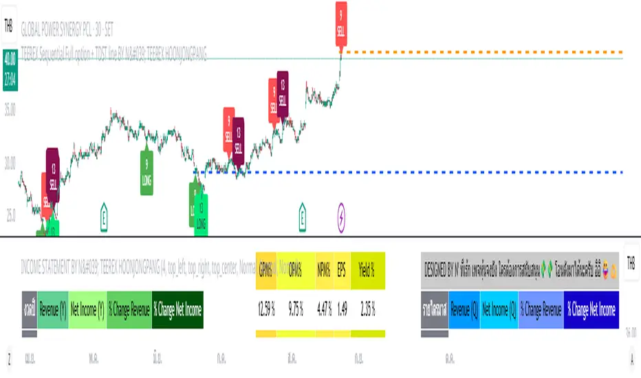
TEEREX COUNTDOWN BY N' TEEREX HOONJONGPANG Features:
Price Flip Detection – identifies initial buy/sell setups based on close price comparisons to previous bars.
Setup Phase (1–9) – counts consecutive bars fulfilling Teerex number conditions; plots numbers on each candle.
Cd Phase (1–13) – continues counting after Setup 9; highlights potential reversal points.
Signals – marks Setup 9 and Countdown 13 with clear labels and arrows (“LONG” / “SELL”).
TDST Lines – draws dynamic support (Buy TDST) or resistance (Sell TDST) lines based on Setup 9 highs/lows. These lines help identify potential breakout or bounce zones.
Customizable Display – options to show/hide numbers, signals, and TDST lines; color-coded for clarity.
Usage:
Monitor Setup 9 and Countdown 13 labels for strong buy/sell signals.
Use TDST lines as reference for support/resistance, target levels, or confirmation of trend continuation.
Visuals:
Numbers 1–9/1–13 appear on the chart for precise counting.
Arrows and labels indicate Setup 9 completion and Cd 13 completion.
TDST lines extend to the right, updating with each new Setup 9.
Markov Chain [3D] | FractalystWhat exactly is a Markov Chain?
This indicator uses a Markov Chain model to analyze, quantify, and visualize the transitions between market regimes (Bull, Bear, Neutral) on your chart. It dynamically detects these regimes in real-time, calculates transition probabilities, and displays them as animated 3D spheres and arrows, giving traders intuitive insight into current and future market conditions.
How does a Markov Chain work, and how should I read this spheres-and-arrows diagram?
Think of three weather modes: Sunny, Rainy, Cloudy.
Each sphere is one mode. The loop on a sphere means “stay the same next step” (e.g., Sunny again tomorrow).
The arrows leaving a sphere show where things usually go next if they change (e.g., Sunny moving to Cloudy).
Some paths matter more than others. A more prominent loop means the current mode tends to persist. A more prominent outgoing arrow means a change to that destination is the usual next step.
Direction isn’t symmetric: moving Sunny→Cloudy can behave differently than Cloudy→Sunny.
Now relabel the spheres to markets: Bull, Bear, Neutral.
Spheres: market regimes (uptrend, downtrend, range).
Self‑loop: tendency for the current regime to continue on the next bar.
Arrows: the most common next regime if a switch happens.
How to read: Start at the sphere that matches current bar state. If the loop stands out, expect continuation. If one outgoing path stands out, that switch is the typical next step. Opposite directions can differ (Bear→Neutral doesn’t have to match Neutral→Bear).
What states and transitions are shown?
The three market states visualized are:
Bullish (Bull): Upward or strong-market regime.
Bearish (Bear): Downward or weak-market regime.
Neutral: Sideways or range-bound regime.
Bidirectional animated arrows and probability labels show how likely the market is to move from one regime to another (e.g., Bull → Bear or Neutral → Bull).
How does the regime detection system work?
You can use either built-in price returns (based on adaptive Z-score normalization) or supply three custom indicators (such as volume, oscillators, etc.).
Values are statistically normalized (Z-scored) over a configurable lookback period.
The normalized outputs are classified into Bull, Bear, or Neutral zones.
If using three indicators, their regime signals are averaged and smoothed for robustness.
How are transition probabilities calculated?
On every confirmed bar, the algorithm tracks the sequence of detected market states, then builds a rolling window of transitions.
The code maintains a transition count matrix for all regime pairs (e.g., Bull → Bear).
Transition probabilities are extracted for each possible state change using Laplace smoothing for numerical stability, and frequently updated in real-time.
What is unique about the visualization?
3D animated spheres represent each regime and change visually when active.
Animated, bidirectional arrows reveal transition probabilities and allow you to see both dominant and less likely regime flows.
Particles (moving dots) animate along the arrows, enhancing the perception of regime flow direction and speed.
All elements dynamically update with each new price bar, providing a live market map in an intuitive, engaging format.
Can I use custom indicators for regime classification?
Yes! Enable the "Custom Indicators" switch and select any three chart series as inputs. These will be normalized and combined (each with equal weight), broadening the regime classification beyond just price-based movement.
What does the “Lookback Period” control?
Lookback Period (default: 100) sets how much historical data builds the probability matrix. Shorter periods adapt faster to regime changes but may be noisier. Longer periods are more stable but slower to adapt.
How is this different from a Hidden Markov Model (HMM)?
It sets the window for both regime detection and probability calculations. Lower values make the system more reactive, but potentially noisier. Higher values smooth estimates and make the system more robust.
How is this Markov Chain different from a Hidden Markov Model (HMM)?
Markov Chain (as here): All market regimes (Bull, Bear, Neutral) are directly observable on the chart. The transition matrix is built from actual detected regimes, keeping the model simple and interpretable.
Hidden Markov Model: The actual regimes are unobservable ("hidden") and must be inferred from market output or indicator "emissions" using statistical learning algorithms. HMMs are more complex, can capture more subtle structure, but are harder to visualize and require additional machine learning steps for training.
A standard Markov Chain models transitions between observable states using a simple transition matrix, while a Hidden Markov Model assumes the true states are hidden (latent) and must be inferred from observable “emissions” like price or volume data. In practical terms, a Markov Chain is transparent and easier to implement and interpret; an HMM is more expressive but requires statistical inference to estimate hidden states from data.
Markov Chain: states are observable; you directly count or estimate transition probabilities between visible states. This makes it simpler, faster, and easier to validate and tune.
HMM: states are hidden; you only observe emissions generated by those latent states. Learning involves machine learning/statistical algorithms (commonly Baum–Welch/EM for training and Viterbi for decoding) to infer both the transition dynamics and the most likely hidden state sequence from data.
How does the indicator avoid “repainting” or look-ahead bias?
All regime changes and matrix updates happen only on confirmed (closed) bars, so no future data is leaked, ensuring reliable real-time operation.
Are there practical tuning tips?
Tune the Lookback Period for your asset/timeframe: shorter for fast markets, longer for stability.
Use custom indicators if your asset has unique regime drivers.
Watch for rapid changes in transition probabilities as early warning of a possible regime shift.
Who is this indicator for?
Quants and quantitative researchers exploring probabilistic market modeling, especially those interested in regime-switching dynamics and Markov models.
Programmers and system developers who need a probabilistic regime filter for systematic and algorithmic backtesting:
The Markov Chain indicator is ideally suited for programmatic integration via its bias output (1 = Bull, 0 = Neutral, -1 = Bear).
Although the visualization is engaging, the core output is designed for automated, rules-based workflows—not for discretionary/manual trading decisions.
Developers can connect the indicator’s output directly to their Pine Script logic (using input.source()), allowing rapid and robust backtesting of regime-based strategies.
It acts as a plug-and-play regime filter: simply plug the bias output into your entry/exit logic, and you have a scientifically robust, probabilistically-derived signal for filtering, timing, position sizing, or risk regimes.
The MC's output is intentionally "trinary" (1/0/-1), focusing on clear regime states for unambiguous decision-making in code. If you require nuanced, multi-probability or soft-label state vectors, consider expanding the indicator or stacking it with a probability-weighted logic layer in your scripting.
Because it avoids subjectivity, this approach is optimal for systematic quants, algo developers building backtested, repeatable strategies based on probabilistic regime analysis.
What's the mathematical foundation behind this?
The mathematical foundation behind this Markov Chain indicator—and probabilistic regime detection in finance—draws from two principal models: the (standard) Markov Chain and the Hidden Markov Model (HMM).
How to use this indicator programmatically?
The Markov Chain indicator automatically exports a bias value (+1 for Bullish, -1 for Bearish, 0 for Neutral) as a plot visible in the Data Window. This allows you to integrate its regime signal into your own scripts and strategies for backtesting, automation, or live trading.
Step-by-Step Integration with Pine Script (input.source)
Add the Markov Chain indicator to your chart.
This must be done first, since your custom script will "pull" the bias signal from the indicator's plot.
In your strategy, create an input using input.source()
Example:
//@version=5
strategy("MC Bias Strategy Example")
mcBias = input.source(close, "MC Bias Source")
After saving, go to your script’s settings. For the “MC Bias Source” input, select the plot/output of the Markov Chain indicator (typically its bias plot).
Use the bias in your trading logic
Example (long only on Bull, flat otherwise):
if mcBias == 1
strategy.entry("Long", strategy.long)
else
strategy.close("Long")
For more advanced workflows, combine mcBias with additional filters or trailing stops.
How does this work behind-the-scenes?
TradingView’s input.source() lets you use any plot from another indicator as a real-time, “live” data feed in your own script (source).
The selected bias signal is available to your Pine code as a variable, enabling logical decisions based on regime (trend-following, mean-reversion, etc.).
This enables powerful strategy modularity : decouple regime detection from entry/exit logic, allowing fast experimentation without rewriting core signal code.
Integrating 45+ Indicators with Your Markov Chain — How & Why
The Enhanced Custom Indicators Export script exports a massive suite of over 45 technical indicators—ranging from classic momentum (RSI, MACD, Stochastic, etc.) to trend, volume, volatility, and oscillator tools—all pre-calculated, centered/scaled, and available as plots.
// Enhanced Custom Indicators Export - 45 Technical Indicators
// Comprehensive technical analysis suite for advanced market regime detection
//@version=6
indicator('Enhanced Custom Indicators Export | Fractalyst', shorttitle='Enhanced CI Export', overlay=false, scale=scale.right, max_labels_count=500, max_lines_count=500)
// |----- Input Parameters -----| //
momentum_group = "Momentum Indicators"
trend_group = "Trend Indicators"
volume_group = "Volume Indicators"
volatility_group = "Volatility Indicators"
oscillator_group = "Oscillator Indicators"
display_group = "Display Settings"
// Common lengths
length_14 = input.int(14, "Standard Length (14)", minval=1, maxval=100, group=momentum_group)
length_20 = input.int(20, "Medium Length (20)", minval=1, maxval=200, group=trend_group)
length_50 = input.int(50, "Long Length (50)", minval=1, maxval=200, group=trend_group)
// Display options
show_table = input.bool(true, "Show Values Table", group=display_group)
table_size = input.string("Small", "Table Size", options= , group=display_group)
// |----- MOMENTUM INDICATORS (15 indicators) -----| //
// 1. RSI (Relative Strength Index)
rsi_14 = ta.rsi(close, length_14)
rsi_centered = rsi_14 - 50
// 2. Stochastic Oscillator
stoch_k = ta.stoch(close, high, low, length_14)
stoch_d = ta.sma(stoch_k, 3)
stoch_centered = stoch_k - 50
// 3. Williams %R
williams_r = ta.stoch(close, high, low, length_14) - 100
// 4. MACD (Moving Average Convergence Divergence)
= ta.macd(close, 12, 26, 9)
// 5. Momentum (Rate of Change)
momentum = ta.mom(close, length_14)
momentum_pct = (momentum / close ) * 100
// 6. Rate of Change (ROC)
roc = ta.roc(close, length_14)
// 7. Commodity Channel Index (CCI)
cci = ta.cci(close, length_20)
// 8. Money Flow Index (MFI)
mfi = ta.mfi(close, length_14)
mfi_centered = mfi - 50
// 9. Awesome Oscillator (AO)
ao = ta.sma(hl2, 5) - ta.sma(hl2, 34)
// 10. Accelerator Oscillator (AC)
ac = ao - ta.sma(ao, 5)
// 11. Chande Momentum Oscillator (CMO)
cmo = ta.cmo(close, length_14)
// 12. Detrended Price Oscillator (DPO)
dpo = close - ta.sma(close, length_20)
// 13. Price Oscillator (PPO)
ppo = ta.sma(close, 12) - ta.sma(close, 26)
ppo_pct = (ppo / ta.sma(close, 26)) * 100
// 14. TRIX
trix_ema1 = ta.ema(close, length_14)
trix_ema2 = ta.ema(trix_ema1, length_14)
trix_ema3 = ta.ema(trix_ema2, length_14)
trix = ta.roc(trix_ema3, 1) * 10000
// 15. Klinger Oscillator
klinger = ta.ema(volume * (high + low + close) / 3, 34) - ta.ema(volume * (high + low + close) / 3, 55)
// 16. Fisher Transform
fisher_hl2 = 0.5 * (hl2 - ta.lowest(hl2, 10)) / (ta.highest(hl2, 10) - ta.lowest(hl2, 10)) - 0.25
fisher = 0.5 * math.log((1 + fisher_hl2) / (1 - fisher_hl2))
// 17. Stochastic RSI
stoch_rsi = ta.stoch(rsi_14, rsi_14, rsi_14, length_14)
stoch_rsi_centered = stoch_rsi - 50
// 18. Relative Vigor Index (RVI)
rvi_num = ta.swma(close - open)
rvi_den = ta.swma(high - low)
rvi = rvi_den != 0 ? rvi_num / rvi_den : 0
// 19. Balance of Power (BOP)
bop = (close - open) / (high - low)
// |----- TREND INDICATORS (10 indicators) -----| //
// 20. Simple Moving Average Momentum
sma_20 = ta.sma(close, length_20)
sma_momentum = ((close - sma_20) / sma_20) * 100
// 21. Exponential Moving Average Momentum
ema_20 = ta.ema(close, length_20)
ema_momentum = ((close - ema_20) / ema_20) * 100
// 22. Parabolic SAR
sar = ta.sar(0.02, 0.02, 0.2)
sar_trend = close > sar ? 1 : -1
// 23. Linear Regression Slope
lr_slope = ta.linreg(close, length_20, 0) - ta.linreg(close, length_20, 1)
// 24. Moving Average Convergence (MAC)
mac = ta.sma(close, 10) - ta.sma(close, 30)
// 25. Trend Intensity Index (TII)
tii_sum = 0.0
for i = 1 to length_20
tii_sum += close > close ? 1 : 0
tii = (tii_sum / length_20) * 100
// 26. Ichimoku Cloud Components
ichimoku_tenkan = (ta.highest(high, 9) + ta.lowest(low, 9)) / 2
ichimoku_kijun = (ta.highest(high, 26) + ta.lowest(low, 26)) / 2
ichimoku_signal = ichimoku_tenkan > ichimoku_kijun ? 1 : -1
// 27. MESA Adaptive Moving Average (MAMA)
mama_alpha = 2.0 / (length_20 + 1)
mama = ta.ema(close, length_20)
mama_momentum = ((close - mama) / mama) * 100
// 28. Zero Lag Exponential Moving Average (ZLEMA)
zlema_lag = math.round((length_20 - 1) / 2)
zlema_data = close + (close - close )
zlema = ta.ema(zlema_data, length_20)
zlema_momentum = ((close - zlema) / zlema) * 100
// |----- VOLUME INDICATORS (6 indicators) -----| //
// 29. On-Balance Volume (OBV)
obv = ta.obv
// 30. Volume Rate of Change (VROC)
vroc = ta.roc(volume, length_14)
// 31. Price Volume Trend (PVT)
pvt = ta.pvt
// 32. Negative Volume Index (NVI)
nvi = 0.0
nvi := volume < volume ? nvi + ((close - close ) / close ) * nvi : nvi
// 33. Positive Volume Index (PVI)
pvi = 0.0
pvi := volume > volume ? pvi + ((close - close ) / close ) * pvi : pvi
// 34. Volume Oscillator
vol_osc = ta.sma(volume, 5) - ta.sma(volume, 10)
// 35. Ease of Movement (EOM)
eom_distance = high - low
eom_box_height = volume / 1000000
eom = eom_box_height != 0 ? eom_distance / eom_box_height : 0
eom_sma = ta.sma(eom, length_14)
// 36. Force Index
force_index = volume * (close - close )
force_index_sma = ta.sma(force_index, length_14)
// |----- VOLATILITY INDICATORS (10 indicators) -----| //
// 37. Average True Range (ATR)
atr = ta.atr(length_14)
atr_pct = (atr / close) * 100
// 38. Bollinger Bands Position
bb_basis = ta.sma(close, length_20)
bb_dev = 2.0 * ta.stdev(close, length_20)
bb_upper = bb_basis + bb_dev
bb_lower = bb_basis - bb_dev
bb_position = bb_dev != 0 ? (close - bb_basis) / bb_dev : 0
bb_width = bb_dev != 0 ? (bb_upper - bb_lower) / bb_basis * 100 : 0
// 39. Keltner Channels Position
kc_basis = ta.ema(close, length_20)
kc_range = ta.ema(ta.tr, length_20)
kc_upper = kc_basis + (2.0 * kc_range)
kc_lower = kc_basis - (2.0 * kc_range)
kc_position = kc_range != 0 ? (close - kc_basis) / kc_range : 0
// 40. Donchian Channels Position
dc_upper = ta.highest(high, length_20)
dc_lower = ta.lowest(low, length_20)
dc_basis = (dc_upper + dc_lower) / 2
dc_position = (dc_upper - dc_lower) != 0 ? (close - dc_basis) / (dc_upper - dc_lower) : 0
// 41. Standard Deviation
std_dev = ta.stdev(close, length_20)
std_dev_pct = (std_dev / close) * 100
// 42. Relative Volatility Index (RVI)
rvi_up = ta.stdev(close > close ? close : 0, length_14)
rvi_down = ta.stdev(close < close ? close : 0, length_14)
rvi_total = rvi_up + rvi_down
rvi_volatility = rvi_total != 0 ? (rvi_up / rvi_total) * 100 : 50
// 43. Historical Volatility
hv_returns = math.log(close / close )
hv = ta.stdev(hv_returns, length_20) * math.sqrt(252) * 100
// 44. Garman-Klass Volatility
gk_vol = math.log(high/low) * math.log(high/low) - (2*math.log(2)-1) * math.log(close/open) * math.log(close/open)
gk_volatility = math.sqrt(ta.sma(gk_vol, length_20)) * 100
// 45. Parkinson Volatility
park_vol = math.log(high/low) * math.log(high/low)
parkinson = math.sqrt(ta.sma(park_vol, length_20) / (4 * math.log(2))) * 100
// 46. Rogers-Satchell Volatility
rs_vol = math.log(high/close) * math.log(high/open) + math.log(low/close) * math.log(low/open)
rogers_satchell = math.sqrt(ta.sma(rs_vol, length_20)) * 100
// |----- OSCILLATOR INDICATORS (5 indicators) -----| //
// 47. Elder Ray Index
elder_bull = high - ta.ema(close, 13)
elder_bear = low - ta.ema(close, 13)
elder_power = elder_bull + elder_bear
// 48. Schaff Trend Cycle (STC)
stc_macd = ta.ema(close, 23) - ta.ema(close, 50)
stc_k = ta.stoch(stc_macd, stc_macd, stc_macd, 10)
stc_d = ta.ema(stc_k, 3)
stc = ta.stoch(stc_d, stc_d, stc_d, 10)
// 49. Coppock Curve
coppock_roc1 = ta.roc(close, 14)
coppock_roc2 = ta.roc(close, 11)
coppock = ta.wma(coppock_roc1 + coppock_roc2, 10)
// 50. Know Sure Thing (KST)
kst_roc1 = ta.roc(close, 10)
kst_roc2 = ta.roc(close, 15)
kst_roc3 = ta.roc(close, 20)
kst_roc4 = ta.roc(close, 30)
kst = ta.sma(kst_roc1, 10) + 2*ta.sma(kst_roc2, 10) + 3*ta.sma(kst_roc3, 10) + 4*ta.sma(kst_roc4, 15)
// 51. Percentage Price Oscillator (PPO)
ppo_line = ((ta.ema(close, 12) - ta.ema(close, 26)) / ta.ema(close, 26)) * 100
ppo_signal = ta.ema(ppo_line, 9)
ppo_histogram = ppo_line - ppo_signal
// |----- PLOT MAIN INDICATORS -----| //
// Plot key momentum indicators
plot(rsi_centered, title="01_RSI_Centered", color=color.purple, linewidth=1)
plot(stoch_centered, title="02_Stoch_Centered", color=color.blue, linewidth=1)
plot(williams_r, title="03_Williams_R", color=color.red, linewidth=1)
plot(macd_histogram, title="04_MACD_Histogram", color=color.orange, linewidth=1)
plot(cci, title="05_CCI", color=color.green, linewidth=1)
// Plot trend indicators
plot(sma_momentum, title="06_SMA_Momentum", color=color.navy, linewidth=1)
plot(ema_momentum, title="07_EMA_Momentum", color=color.maroon, linewidth=1)
plot(sar_trend, title="08_SAR_Trend", color=color.teal, linewidth=1)
plot(lr_slope, title="09_LR_Slope", color=color.lime, linewidth=1)
plot(mac, title="10_MAC", color=color.fuchsia, linewidth=1)
// Plot volatility indicators
plot(atr_pct, title="11_ATR_Pct", color=color.yellow, linewidth=1)
plot(bb_position, title="12_BB_Position", color=color.aqua, linewidth=1)
plot(kc_position, title="13_KC_Position", color=color.olive, linewidth=1)
plot(std_dev_pct, title="14_StdDev_Pct", color=color.silver, linewidth=1)
plot(bb_width, title="15_BB_Width", color=color.gray, linewidth=1)
// Plot volume indicators
plot(vroc, title="16_VROC", color=color.blue, linewidth=1)
plot(eom_sma, title="17_EOM", color=color.red, linewidth=1)
plot(vol_osc, title="18_Vol_Osc", color=color.green, linewidth=1)
plot(force_index_sma, title="19_Force_Index", color=color.orange, linewidth=1)
plot(obv, title="20_OBV", color=color.purple, linewidth=1)
// Plot additional oscillators
plot(ao, title="21_Awesome_Osc", color=color.navy, linewidth=1)
plot(cmo, title="22_CMO", color=color.maroon, linewidth=1)
plot(dpo, title="23_DPO", color=color.teal, linewidth=1)
plot(trix, title="24_TRIX", color=color.lime, linewidth=1)
plot(fisher, title="25_Fisher", color=color.fuchsia, linewidth=1)
// Plot more momentum indicators
plot(mfi_centered, title="26_MFI_Centered", color=color.yellow, linewidth=1)
plot(ac, title="27_AC", color=color.aqua, linewidth=1)
plot(ppo_pct, title="28_PPO_Pct", color=color.olive, linewidth=1)
plot(stoch_rsi_centered, title="29_StochRSI_Centered", color=color.silver, linewidth=1)
plot(klinger, title="30_Klinger", color=color.gray, linewidth=1)
// Plot trend continuation
plot(tii, title="31_TII", color=color.blue, linewidth=1)
plot(ichimoku_signal, title="32_Ichimoku_Signal", color=color.red, linewidth=1)
plot(mama_momentum, title="33_MAMA_Momentum", color=color.green, linewidth=1)
plot(zlema_momentum, title="34_ZLEMA_Momentum", color=color.orange, linewidth=1)
plot(bop, title="35_BOP", color=color.purple, linewidth=1)
// Plot volume continuation
plot(nvi, title="36_NVI", color=color.navy, linewidth=1)
plot(pvi, title="37_PVI", color=color.maroon, linewidth=1)
plot(momentum_pct, title="38_Momentum_Pct", color=color.teal, linewidth=1)
plot(roc, title="39_ROC", color=color.lime, linewidth=1)
plot(rvi, title="40_RVI", color=color.fuchsia, linewidth=1)
// Plot volatility continuation
plot(dc_position, title="41_DC_Position", color=color.yellow, linewidth=1)
plot(rvi_volatility, title="42_RVI_Volatility", color=color.aqua, linewidth=1)
plot(hv, title="43_Historical_Vol", color=color.olive, linewidth=1)
plot(gk_volatility, title="44_GK_Volatility", color=color.silver, linewidth=1)
plot(parkinson, title="45_Parkinson_Vol", color=color.gray, linewidth=1)
// Plot final oscillators
plot(rogers_satchell, title="46_RS_Volatility", color=color.blue, linewidth=1)
plot(elder_power, title="47_Elder_Power", color=color.red, linewidth=1)
plot(stc, title="48_STC", color=color.green, linewidth=1)
plot(coppock, title="49_Coppock", color=color.orange, linewidth=1)
plot(kst, title="50_KST", color=color.purple, linewidth=1)
// Plot final indicators
plot(ppo_histogram, title="51_PPO_Histogram", color=color.navy, linewidth=1)
plot(pvt, title="52_PVT", color=color.maroon, linewidth=1)
// |----- Reference Lines -----| //
hline(0, "Zero Line", color=color.gray, linestyle=hline.style_dashed, linewidth=1)
hline(50, "Midline", color=color.gray, linestyle=hline.style_dotted, linewidth=1)
hline(-50, "Lower Midline", color=color.gray, linestyle=hline.style_dotted, linewidth=1)
hline(25, "Upper Threshold", color=color.gray, linestyle=hline.style_dotted, linewidth=1)
hline(-25, "Lower Threshold", color=color.gray, linestyle=hline.style_dotted, linewidth=1)
// |----- Enhanced Information Table -----| //
if show_table and barstate.islast
table_position = position.top_right
table_text_size = table_size == "Tiny" ? size.tiny : table_size == "Small" ? size.small : size.normal
var table info_table = table.new(table_position, 3, 18, bgcolor=color.new(color.white, 85), border_width=1, border_color=color.gray)
// Headers
table.cell(info_table, 0, 0, 'Category', text_color=color.black, text_size=table_text_size, bgcolor=color.new(color.blue, 70))
table.cell(info_table, 1, 0, 'Indicator', text_color=color.black, text_size=table_text_size, bgcolor=color.new(color.blue, 70))
table.cell(info_table, 2, 0, 'Value', text_color=color.black, text_size=table_text_size, bgcolor=color.new(color.blue, 70))
// Key Momentum Indicators
table.cell(info_table, 0, 1, 'MOMENTUM', text_color=color.purple, text_size=table_text_size, bgcolor=color.new(color.purple, 90))
table.cell(info_table, 1, 1, 'RSI Centered', text_color=color.purple, text_size=table_text_size)
table.cell(info_table, 2, 1, str.tostring(rsi_centered, '0.00'), text_color=color.purple, text_size=table_text_size)
table.cell(info_table, 0, 2, '', text_color=color.blue, text_size=table_text_size)
table.cell(info_table, 1, 2, 'Stoch Centered', text_color=color.blue, text_size=table_text_size)
table.cell(info_table, 2, 2, str.tostring(stoch_centered, '0.00'), text_color=color.blue, text_size=table_text_size)
table.cell(info_table, 0, 3, '', text_color=color.red, text_size=table_text_size)
table.cell(info_table, 1, 3, 'Williams %R', text_color=color.red, text_size=table_text_size)
table.cell(info_table, 2, 3, str.tostring(williams_r, '0.00'), text_color=color.red, text_size=table_text_size)
table.cell(info_table, 0, 4, '', text_color=color.orange, text_size=table_text_size)
table.cell(info_table, 1, 4, 'MACD Histogram', text_color=color.orange, text_size=table_text_size)
table.cell(info_table, 2, 4, str.tostring(macd_histogram, '0.000'), text_color=color.orange, text_size=table_text_size)
table.cell(info_table, 0, 5, '', text_color=color.green, text_size=table_text_size)
table.cell(info_table, 1, 5, 'CCI', text_color=color.green, text_size=table_text_size)
table.cell(info_table, 2, 5, str.tostring(cci, '0.00'), text_color=color.green, text_size=table_text_size)
// Key Trend Indicators
table.cell(info_table, 0, 6, 'TREND', text_color=color.navy, text_size=table_text_size, bgcolor=color.new(color.navy, 90))
table.cell(info_table, 1, 6, 'SMA Momentum %', text_color=color.navy, text_size=table_text_size)
table.cell(info_table, 2, 6, str.tostring(sma_momentum, '0.00'), text_color=color.navy, text_size=table_text_size)
table.cell(info_table, 0, 7, '', text_color=color.maroon, text_size=table_text_size)
table.cell(info_table, 1, 7, 'EMA Momentum %', text_color=color.maroon, text_size=table_text_size)
table.cell(info_table, 2, 7, str.tostring(ema_momentum, '0.00'), text_color=color.maroon, text_size=table_text_size)
table.cell(info_table, 0, 8, '', text_color=color.teal, text_size=table_text_size)
table.cell(info_table, 1, 8, 'SAR Trend', text_color=color.teal, text_size=table_text_size)
table.cell(info_table, 2, 8, str.tostring(sar_trend, '0'), text_color=color.teal, text_size=table_text_size)
table.cell(info_table, 0, 9, '', text_color=color.lime, text_size=table_text_size)
table.cell(info_table, 1, 9, 'Linear Regression', text_color=color.lime, text_size=table_text_size)
table.cell(info_table, 2, 9, str.tostring(lr_slope, '0.000'), text_color=color.lime, text_size=table_text_size)
// Key Volatility Indicators
table.cell(info_table, 0, 10, 'VOLATILITY', text_color=color.yellow, text_size=table_text_size, bgcolor=color.new(color.yellow, 90))
table.cell(info_table, 1, 10, 'ATR %', text_color=color.yellow, text_size=table_text_size)
table.cell(info_table, 2, 10, str.tostring(atr_pct, '0.00'), text_color=color.yellow, text_size=table_text_size)
table.cell(info_table, 0, 11, '', text_color=color.aqua, text_size=table_text_size)
table.cell(info_table, 1, 11, 'BB Position', text_color=color.aqua, text_size=table_text_size)
table.cell(info_table, 2, 11, str.tostring(bb_position, '0.00'), text_color=color.aqua, text_size=table_text_size)
table.cell(info_table, 0, 12, '', text_color=color.olive, text_size=table_text_size)
table.cell(info_table, 1, 12, 'KC Position', text_color=color.olive, text_size=table_text_size)
table.cell(info_table, 2, 12, str.tostring(kc_position, '0.00'), text_color=color.olive, text_size=table_text_size)
// Key Volume Indicators
table.cell(info_table, 0, 13, 'VOLUME', text_color=color.blue, text_size=table_text_size, bgcolor=color.new(color.blue, 90))
table.cell(info_table, 1, 13, 'Volume ROC', text_color=color.blue, text_size=table_text_size)
table.cell(info_table, 2, 13, str.tostring(vroc, '0.00'), text_color=color.blue, text_size=table_text_size)
table.cell(info_table, 0, 14, '', text_color=color.red, text_size=table_text_size)
table.cell(info_table, 1, 14, 'EOM', text_color=color.red, text_size=table_text_size)
table.cell(info_table, 2, 14, str.tostring(eom_sma, '0.000'), text_color=color.red, text_size=table_text_size)
// Key Oscillators
table.cell(info_table, 0, 15, 'OSCILLATORS', text_color=color.purple, text_size=table_text_size, bgcolor=color.new(color.purple, 90))
table.cell(info_table, 1, 15, 'Awesome Osc', text_color=color.blue, text_size=table_text_size)
table.cell(info_table, 2, 15, str.tostring(ao, '0.000'), text_color=color.blue, text_size=table_text_size)
table.cell(info_table, 0, 16, '', text_color=color.red, text_size=table_text_size)
table.cell(info_table, 1, 16, 'Fisher Transform', text_color=color.red, text_size=table_text_size)
table.cell(info_table, 2, 16, str.tostring(fisher, '0.000'), text_color=color.red, text_size=table_text_size)
// Summary Statistics
table.cell(info_table, 0, 17, 'SUMMARY', text_color=color.black, text_size=table_text_size, bgcolor=color.new(color.gray, 70))
table.cell(info_table, 1, 17, 'Total Indicators: 52', text_color=color.black, text_size=table_text_size)
regime_color = rsi_centered > 10 ? color.green : rsi_centered < -10 ? color.red : color.gray
regime_text = rsi_centered > 10 ? "BULLISH" : rsi_centered < -10 ? "BEARISH" : "NEUTRAL"
table.cell(info_table, 2, 17, regime_text, text_color=regime_color, text_size=table_text_size)
This makes it the perfect “indicator backbone” for quantitative and systematic traders who want to prototype, combine, and test new regime detection models—especially in combination with the Markov Chain indicator.
How to use this script with the Markov Chain for research and backtesting:
Add the Enhanced Indicator Export to your chart.
Every calculated indicator is available as an individual data stream.
Connect the indicator(s) you want as custom input(s) to the Markov Chain’s “Custom Indicators” option.
In the Markov Chain indicator’s settings, turn ON the custom indicator mode.
For each of the three custom indicator inputs, select the exported plot from the Enhanced Export script—the menu lists all 45+ signals by name.
This creates a powerful, modular regime-detection engine where you can mix-and-match momentum, trend, volume, or custom combinations for advanced filtering.
Backtest regime logic directly.
Once you’ve connected your chosen indicators, the Markov Chain script performs regime detection (Bull/Neutral/Bear) based on your selected features—not just price returns.
The regime detection is robust, automatically normalized (using Z-score), and outputs bias (1, -1, 0) for plug-and-play integration.
Export the regime bias for programmatic use.
As described above, use input.source() in your Pine Script strategy or system and link the bias output.
You can now filter signals, control trade direction/size, or design pairs-trading that respect true, indicator-driven market regimes.
With this framework, you’re not limited to static or simplistic regime filters. You can rigorously define, test, and refine what “market regime” means for your strategies—using the technical features that matter most to you.
Optimize your signal generation by backtesting across a universe of meaningful indicator blends.
Enhance risk management with objective, real-time regime boundaries.
Accelerate your research: iterate quickly, swap indicator components, and see results with minimal code changes.
Automate multi-asset or pairs-trading by integrating regime context directly into strategy logic.
Add both scripts to your chart, connect your preferred features, and start investigating your best regime-based trades—entirely within the TradingView ecosystem.
References & Further Reading
Ang, A., & Bekaert, G. (2002). “Regime Switches in Interest Rates.” Journal of Business & Economic Statistics, 20(2), 163–182.
Hamilton, J. D. (1989). “A New Approach to the Economic Analysis of Nonstationary Time Series and the Business Cycle.” Econometrica, 57(2), 357–384.
Markov, A. A. (1906). "Extension of the Limit Theorems of Probability Theory to a Sum of Variables Connected in a Chain." The Notes of the Imperial Academy of Sciences of St. Petersburg.
Guidolin, M., & Timmermann, A. (2007). “Asset Allocation under Multivariate Regime Switching.” Journal of Economic Dynamics and Control, 31(11), 3503–3544.
Murphy, J. J. (1999). Technical Analysis of the Financial Markets. New York Institute of Finance.
Brock, W., Lakonishok, J., & LeBaron, B. (1992). “Simple Technical Trading Rules and the Stochastic Properties of Stock Returns.” Journal of Finance, 47(5), 1731–1764.
Zucchini, W., MacDonald, I. L., & Langrock, R. (2017). Hidden Markov Models for Time Series: An Introduction Using R (2nd ed.). Chapman and Hall/CRC.
On Quantitative Finance and Markov Models:
Lo, A. W., & Hasanhodzic, J. (2009). The Heretics of Finance: Conversations with Leading Practitioners of Technical Analysis. Bloomberg Press.
Patterson, S. (2016). The Man Who Solved the Market: How Jim Simons Launched the Quant Revolution. Penguin Press.
TradingView Pine Script Documentation: www.tradingview.com
TradingView Blog: “Use an Input From Another Indicator With Your Strategy” www.tradingview.com
GeeksforGeeks: “What is the Difference Between Markov Chains and Hidden Markov Models?” www.geeksforgeeks.org
What makes this indicator original and unique?
- On‑chart, real‑time Markov. The chain is drawn directly on your chart. You see the current regime, its tendency to stay (self‑loop), and the usual next step (arrows) as bars confirm.
- Source‑agnostic by design. The engine runs on any series you select via input.source() — price, your own oscillator, a composite score, anything you compute in the script.
- Automatic normalization + regime mapping. Different inputs live on different scales. The script standardizes your chosen source and maps it into clear regimes (e.g., Bull / Bear / Neutral) without you micromanaging thresholds each time.
- Rolling, bar‑by‑bar learning. Transition tendencies are computed from a rolling window of confirmed bars. What you see is exactly what the market did in that window.
- Fast experimentation. Switch the source, adjust the window, and the Markov view updates instantly. It’s a rapid way to test ideas and feel regime persistence/switch behavior.
Integrate your own signals (using input.source())
- In settings, choose the Source . This is powered by input.source() .
- Feed it price, an indicator you compute inside the script, or a custom composite series.
- The script will automatically normalize that series and process it through the Markov engine, mapping it to regimes and updating the on‑chart spheres/arrows in real time.
Credits:
Deep gratitude to @RicardoSantos for both the foundational Markov chain processing engine and inspiring open-source contributions, which made advanced probabilistic market modeling accessible to the TradingView community.
Special thanks to @Alien_Algorithms for the innovative and visually stunning 3D sphere logic that powers the indicator’s animated, regime-based visualization.
Disclaimer
This tool summarizes recent behavior. It is not financial advice and not a guarantee of future results.

SCTI V30Description
The SCTI V30 is an advanced multi-functional technical analysis indicator for TradingView that combines multiple analytical approaches into a single comprehensive tool. This indicator provides:
Multiple Moving Average Types (EMA, SMA, PMA with various calculation methods)
Customizable VWAP with standard deviation bands
Sophisticated Divergence Detection across 12 different indicators
Volume Profile Analysis with peak/trough detection
Highly Configurable Display Options
The indicator is designed to help traders identify trends, potential reversals, and key support/resistance levels across different timeframes.
Features
1. Moving Average Systems
EMA Section: 13 configurable EMA periods (8, 13, 21, 34, 55, 89, 144, 233, 377, 610, 987, 1597, 2584)
SMA Section: 13 configurable SMA periods (same as EMA)
PMA Section: 11 customizable moving averages with multiple calculation methods:
ALMA, EMA, RMA, SMA, SWMA, VWAP, VWMA, WMA
Adjustable lengths from 12 to 1056
Customizable colors, widths, and fill options between MAs
2. VWAP Implementation
Multiple anchor periods (Session, Week, Month, Quarter, Year, etc.)
Standard deviation or percentage-based bands
Option to hide on daily/weekly/monthly timeframes
Customizable band multipliers (1.0, 2.0, 3.0)
3. Divergence Detection
Detects regular and hidden divergences across 12 indicators:
MACD, MACD Histogram, RSI, Stochastic, CCI, Momentum
OBV, VW-MACD, Chaikin Money Flow, Money Flow Index
Williams %R, and custom external indicators
Customizable detection parameters:
Pivot point period (1-50)
Source (Close or High/Low)
Divergence type (Regular, Hidden, or Both)
Minimum number of divergences required (1-11)
Maximum pivot points to check (1-20)
Maximum bars to look back (30-200)
4. Volume Profile Analysis
Configurable profile length (10-5000 bars)
Value Area threshold (0-100%)
Profile placement (Left or Right)
Number of rows (30-130)
Profile width adjustment
Volume node detection:
Peaks (with cluster option)
Troughs (with cluster option)
Highest/Lowest volume nodes
Customizable colors for all elements
Input Parameters
The indicator is organized into 7 parameter groups:
Basic Indicator Settings - Toggle visibility of main components
EMA Settings - Configure 13 EMA periods and visibility
SMA Settings - Configure 13 SMA periods and visibility
PMA Settings - Advanced moving average configuration
VWAP Settings - Volume-weighted average price configuration
Divergence Settings - Comprehensive divergence detection options
Volume Profile & Node Detection - Volume analysis configuration
How to Use
Trend Identification: Use the multiple moving averages to identify trend direction and strength. The Fibonacci-based periods (21, 34, 55, 89, 144, etc.) are particularly useful for this.
Support/Resistance: The VWAP and volume profile components help identify key support/resistance levels.
Divergence Trading: Look for divergences between price and the various indicators to spot potential reversal points.
Volume Analysis: The volume profile shows where the most trading activity occurred, highlighting important price levels.
Customization: Adjust the settings to match your trading style and timeframe. The indicator is highly configurable to suit different trading approaches.
Alerts
The indicator includes alert conditions for:
Positive regular divergence detected
Negative regular divergence detected
Positive hidden divergence detected
Negative hidden divergence detected
Any positive divergence (regular or hidden)
Any negative divergence (regular or hidden)
Notes
The indicator may be resource-intensive due to its comprehensive calculations, especially on lower timeframes with long lookback periods.
Some features (like VWAP) can be hidden on higher timeframes to improve performance.
The default settings are optimized for daily charts but can be adjusted for any timeframe.
This powerful all-in-one indicator provides traders with a complete toolkit for technical analysis, combining trend-following, momentum, volume, and divergence techniques into a single, customizable solution.
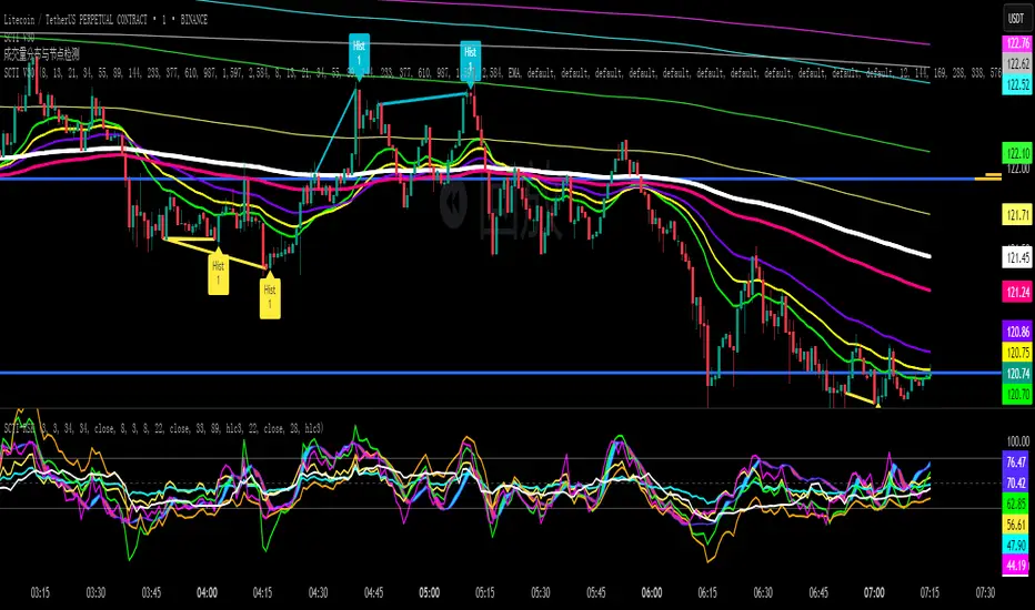
Multi-Confluence Swing Hunter V1# Multi-Confluence Swing Hunter V1 - Complete Description
Overview
The Multi-Confluence Swing Hunter V1 is a sophisticated low timeframe scalping strategy specifically optimized for MSTR (MicroStrategy) trading. This strategy employs a comprehensive point-based scoring system that combines optimized technical indicators, price action analysis, and reversal pattern recognition to generate precise trading signals on lower timeframes.
Performance Highlight:
In backtesting on MSTR 5-minute charts, this strategy has demonstrated over 200% profit performance, showcasing its effectiveness in capturing rapid price movements and volatility patterns unique to MicroStrategy's trading behavior.
The strategy's parameters have been fine-tuned for MSTR's unique volatility characteristics, though they can be optimized for other high-volatility instruments as well.
## Key Innovation & Originality
This strategy introduces a unique **dual scoring system** approach:
- **Entry Scoring**: Identifies swing bottoms using 13+ different technical criteria
- **Exit Scoring**: Identifies swing tops using inverse criteria for optimal exit timing
Unlike traditional strategies that rely on simple indicator crossovers, this system quantifies market conditions through a weighted scoring mechanism, providing objective, data-driven entry and exit decisions.
## Technical Foundation
### Optimized Indicator Parameters
The strategy utilizes extensively backtested parameters specifically optimized for MSTR's volatility patterns:
**MACD Configuration (3,10,3)**:
- Fast EMA: 3 periods (vs standard 12)
- Slow EMA: 10 periods (vs standard 26)
- Signal Line: 3 periods (vs standard 9)
- **Rationale**: These faster parameters provide earlier signal detection while maintaining reliability, particularly effective for MSTR's rapid price movements and high-frequency volatility
**RSI Configuration (21-period)**:
- Length: 21 periods (vs standard 14)
- Oversold: 30 level
- Extreme Oversold: 25 level
- **Rationale**: The 21-period RSI reduces false signals while still capturing oversold conditions effectively in MSTR's volatile environment
**Parameter Adaptability**: While optimized for MSTR, these parameters can be adjusted for other high-volatility instruments. Faster-moving stocks may benefit from even shorter MACD periods, while less volatile assets might require longer periods for optimal performance.
### Scoring System Methodology
**Entry Score Components (Minimum 13 points required)**:
1. **RSI Signals** (max 5 points):
- RSI < 30: +2 points
- RSI < 25: +2 points
- RSI turning up: +1 point
2. **MACD Signals** (max 8 points):
- MACD below zero: +1 point
- MACD turning up: +2 points
- MACD histogram improving: +2 points
- MACD bullish divergence: +3 points
3. **Price Action** (max 4 points):
- Long lower wick (>50%): +2 points
- Small body (<30%): +1 point
- Bullish close: +1 point
4. **Pattern Recognition** (max 8 points):
- RSI bullish divergence: +4 points
- Quick recovery pattern: +2 points
- Reversal confirmation: +4 points
**Exit Score Components (Minimum 13 points required)**:
Uses inverse criteria to identify swing tops with similar weighting system.
## Risk Management Features
### Position Sizing & Risk Control
- **Single Position Strategy**: 100% equity allocation per trade
- **No Overlapping Positions**: Ensures focused risk management
- **Configurable Risk/Reward**: Default 5:1 ratio optimized for volatile assets
### Stop Loss & Take Profit Logic
- **Dynamic Stop Loss**: Based on recent swing lows with configurable buffer
- **Risk-Based Take Profit**: Calculated using risk/reward ratio
- **Clean Exit Logic**: Prevents conflicting signals
## Default Settings Optimization
### Key Parameters (Optimized for MSTR/Bitcoin-style volatility):
- **Minimum Entry Score**: 13 (ensures high-conviction entries)
- **Minimum Exit Score**: 13 (prevents premature exits)
- **Risk/Reward Ratio**: 5.0 (accounts for volatility)
- **Lower Wick Threshold**: 50% (identifies true hammer patterns)
- **Divergence Lookback**: 8 bars (optimal for swing timeframes)
### Why These Defaults Work for MSTR:
1. **Higher Score Thresholds**: MSTR's volatility requires more confirmation
2. **5:1 Risk/Reward**: Compensates for wider stops needed in volatile markets
3. **Faster MACD**: Captures momentum shifts quickly in fast-moving stocks
4. **21-period RSI**: Reduces noise while maintaining sensitivity
## Visual Features
### Score Display System
- **Green Labels**: Entry scores ≥10 points (below bars)
- **Red Labels**: Exit scores ≥10 points (above bars)
- **Large Triangles**: Actual trade entries/exits
- **Small Triangles**: Reversal pattern confirmations
### Chart Cleanliness
- Indicators plotted in separate panes (MACD, RSI)
- TP/SL levels shown only during active positions
- Clear trade markers distinguish signals from actual trades
## Backtesting Specifications
### Realistic Trading Conditions
- **Commission**: 0.1% per trade
- **Slippage**: 3 points
- **Initial Capital**: $1,000
- **Account Type**: Cash (no margin)
### Sample Size Considerations
- Strategy designed for 100+ trade sample sizes
- Recommended timeframes: 4H, 1D for swing trading
- Optimal for trending/volatile markets
## Strategy Limitations & Considerations
### Market Conditions
- **Best Performance**: Trending markets with clear swings
- **Reduced Effectiveness**: Highly choppy, sideways markets
- **Volatility Dependency**: Optimized for moderate to high volatility assets
### Risk Warnings
- **High Allocation**: 100% position sizing increases risk
- **No Diversification**: Single position strategy
- **Backtesting Limitation**: Past performance doesn't guarantee future results
## Usage Guidelines
### Recommended Assets & Timeframes
- **Primary Target**: MSTR (MicroStrategy) - 5min to 15min timeframes
- **Secondary Targets**: High-volatility stocks (TSLA, NVDA, COIN, etc.)
- **Crypto Markets**: Bitcoin, Ethereum (with parameter adjustments)
- **Timeframe Optimization**: 1min-15min for scalping, 30min-1H for swing scalping
### Timeframe Recommendations
- **Primary Scalping**: 5-minute and 15-minute charts
- **Active Monitoring**: 1-minute for precise entries
- **Swing Scalping**: 30-minute to 1-hour timeframes
- **Avoid**: Sub-1-minute (excessive noise) and above 4-hour (reduces scalping opportunities)
## Technical Requirements
- **Pine Script Version**: v6
- **Overlay**: Yes (plots on price chart)
- **Additional Panes**: MACD and RSI indicators
- **Real-time Compatibility**: Confirmed bar signals only
## Customization Options
All parameters are fully customizable through inputs:
- Indicator lengths and levels
- Scoring thresholds
- Risk management settings
- Visual display preferences
- Date range filtering
## Conclusion
This scalping strategy represents a comprehensive approach to low timeframe trading that combines multiple technical analysis methods into a cohesive, quantified system specifically optimized for MSTR's unique volatility characteristics. The optimized parameters and scoring methodology provide a systematic way to identify high-probability scalping setups while managing risk effectively in fast-moving markets.
The strategy's strength lies in its objective, multi-criteria approach that removes emotional decision-making from scalping while maintaining the flexibility to adapt to different instruments through parameter optimization. While designed for MSTR, the underlying methodology can be fine-tuned for other high-volatility assets across various markets.
**Important Disclaimer**: This strategy is designed for experienced scalpers and is optimized for MSTR trading. The high-frequency nature of scalping involves significant risk. Past performance does not guarantee future results. Always conduct your own analysis, consider your risk tolerance, and be aware of commission/slippage costs that can significantly impact scalping profitability.

Reversal Knockout v1.1\ Reversal Knockout v1.1 — User Manual \
Reversal Knockout is a technical indicator designed to detect potential price turning points using a dual approach: a reversal logic with bar coloring and a combined sequence of setups, countdowns, and exhaustion patterns.
\ What does this indicator do?\
\ Colors candles\ based on the relationship between two smoothed moving averages (T3).
\ Identifies overextension conditions\ based on a sequence of 9 consecutive closes aligned with price direction.
\ Confirms exhaustion\ if, after that setup, 13 follow-through conditions (countdown) are met.
\ Highlights special signals called “Knockouts”\ , which represent strong potential reversal scenarios.
\ Candle Coloring\
Candles are automatically colored to make trend and potential reversal points visually easier to interpret:
🔵 Bull Trend: User-defined color (default light blue)
🔴 Bear Trend: User-defined color (default light red)
🟡 Bullish Reversal: When price crosses below the slower average (default yellow)
🟡 Bearish Reversal: When price crosses above the slower average (default yellow)
This logic is based on the relationship between two T3 moving averages (one fast, one slow), calculated with a customizable smoothing factor.
\ Setup and Countdown Logic\
Setups (9):
A bullish setup forms if the price closes below the close from 4 bars earlier for 9 consecutive candles.
A bearish setup forms if the price closes above the close from 4 bars earlier for 9 consecutive candles.
When the ninth close is completed, a green “9” (buy) or purple “9” (sell) is displayed.
Countdowns (13):
After a setup, a follow-through phase begins.
If 13 additional conditions are met (price < low\ for buys or > high\ for sells), a purple “13” is shown, signaling potential exhaustion.
\ Knockout: Explosive Reversal Potential\
The indicator also identifies special reversal patterns called \ Knockout\ .
These signals appear when, in addition to a “9”, the price shows technical excess behavior near key support or resistance zones:
Knockout ▲ (buy): Appears below the candle when a buy signal is detected with specific downside pressure conditions.
Knockout ▼ (sell): Appears above the candle when a sell signal is detected with upside pressure conditions.
These signals stand out as high-probability reversal opportunities.
\ Usage Recommendations\
The indicator is designed to work on any timeframe, but it is recommended to use it alongside market structure and volume analysis.
“Knockout” signals may be used as high-probability trend change alerts, especially after a “13”.
Can be combined with momentum indicators and moving averages for greater effectiveness.

Quarterly Theory ICT 02 [TradingFinder] True Open Session 90 Min🔵 Introduction
The Quarterly Theory ICT indicator is an advanced analytical system built on ICT (Inner Circle Trader) concepts and fractal time. It divides time into four quarters (Q1, Q2, Q3, Q4), and is designed based on the consistent repetition of these phases across all trading timeframes (annual, monthly, weekly, daily, and even shorter trading sessions).
Each cycle consists of four distinct phases: the first phase (Q1) is the Accumulation phase, characterized by price consolidation; the second phase (Q2), known as Manipulation or Judas Swing, is marked by initial false movements indicating a potential shift; the third phase (Q3) is Distribution, where price volatility peaks; and the fourth phase (Q4) is Continuation/Reversal, determining whether the previous trend continues or reverses.
🔵 How to Use
The central concept of this strategy is the "True Open," which refers to the actual starting point of each time cycle. The True Open is typically defined at the beginning of the second phase (Q2) of each cycle. Prices trading above or below the True Open serve as a benchmark for predicting the market's potential direction and guiding trading decisions.
The practical application of the Quarterly Theory strategy relies on accurately identifying True Open points across various timeframes.
True Open points are defined as follows :
Yearly Cycle :
Q1: January, February, March
Q2: April, May, June (True Open: April Monthly Open)
Q3: July, August, September
Q4: October, November, December
Monthly Cycle :
Q1: First Monday of the month
Q2: Second Monday of the month (True Open: Daily Candle Open price on the second Monday)
Q3: Third Monday of the month
Q4: Fourth Monday of the month
Weekly Cycle :
Q1: Monday
Q2: Tuesday (True Open: Daily Candle Open Price on Tuesday)
Q3: Wednesday
Q4: Thursday
Daily Cycle :
Q1: 18:00 - 00:00 (Asian session)
Q2: 00:00 - 06:00 (True Open: Start of London Session)
Q3: 06:00 - 12:00 (NY AM)
Q4: 12:00 - 18:00 (NY PM)
90 Min Asian Session :
Q1: 18:00 - 19:30
Q2: 19:30 - 21:00 (True Open at 19:30)
Q3: 21:00 - 22:30
Q4: 22:30 - 00:00
90 Min London Session :
Q1: 00:00 - 01:30
Q2: 01:30 - 03:00 (True Open at 01:30)
Q3: 03:00 - 04:30
Q4: 04:30 - 06:00
90 Min New York AM Session :
Q1: 06:00 - 07:30
Q2: 07:30 - 09:00 (True Open at 07:30)
Q3: 09:00 - 10:30
Q4: 10:30 - 12:00
90 Min New York PM Session :
Q1: 12:00 - 13:30
Q2: 13:30 - 15:00 (True Open at 13:30)
Q3: 15:00 - 16:30
Q4: 16:30 - 18:00
Micro Cycle (22.5-Minute Quarters) : Each 90-minute quarter is further divided into four 22.5-minute sub-segments (Micro Sessions).
True Opens in these sessions are defined as follows :
Asian Micro Session :
True Session Open : 19:30 - 19:52:30
London Micro Session :
T rue Session Open : 01:30 - 01:52:30
New York AM Micro Session :
True Session Open : 07:30 - 07:52:30
New York PM Micro Session :
True Session Open : 13:30 - 13:52:30
By accurately identifying these True Open points across various timeframes, traders can effectively forecast the market direction, analyze price movements in detail, and optimize their trading positions. Prices trading above or below these key levels serve as critical benchmarks for determining market direction and making informed trading decisions.
🔵 Setting
Show True Range : Enable or disable the display of the True Range on the chart, including the option to customize the color.
Extend True Range Line : Choose how to extend the True Range line on the chart, with the following options:
None: No line extension
Right: Extend the line to the right
Left: Extend the line to the left
Both: Extend the line in both directions (left and right)
Show Table : Determines whether the table—which summarizes the phases (Q1 to Q4)—is displayed.
Show More Info : Adds additional details to the table, such as the name of the phase (Accumulation, Manipulation, Distribution, or Continuation/Reversal) or further specifics about each cycle.
🔵 Conclusion
The Quarterly Theory ICT, by dividing time into four distinct quarters (Q1, Q2, Q3, and Q4) and emphasizing the concept of the True Open, provides a structured and repeatable framework for analyzing price action across multiple time frames.
The consistent repetition of phases—Accumulation, Manipulation (Judas Swing), Distribution, and Continuation/Reversal—allows traders to effectively identify recurring price patterns and critical market turning points. Utilizing the True Open as a benchmark, traders can more accurately determine potential directional bias, optimize trade entries and exits, and manage risk effectively.
By incorporating principles of ICT (Inner Circle Trader) and fractal time, this strategy enhances market forecasting accuracy across annual, monthly, weekly, daily, and shorter trading sessions. This systematic approach helps traders gain deeper insight into market structure and confidently execute informed trading decisions.

Global M2 Index Percentage### **Global M2 Index Percentage**
**Description:**
The **Global M2 Index Percentage** is a custom indicator designed to track and visualize the global money supply (M2) in a normalized percentage format. It aggregates M2 data from major economies (e.g., the US, EU, China, Japan, and the UK) and adjusts for exchange rates to provide a comprehensive view of global liquidity. This indicator helps traders and investors understand the broader macroeconomic environment, identify trends in money supply, and make informed decisions based on global liquidity conditions.
---
### **How It Works:**
1. **Data Aggregation**:
- The indicator collects M2 data from key economies and adjusts it using exchange rates to calculate a global M2 value.
- The formula for global M2 is:
\
2. **Normalization**:
- The global M2 value is normalized into a percentage (0% to 100%) based on its range over a user-defined period (default: 13 weeks).
- The formula for normalization is:
\
3. **Visualization**:
- The indicator plots the M2 Index as a line chart.
- Key reference levels are highlighted:
- **10% (Red Line)**: Oversold level (low liquidity).
- **50% (Black Line)**: Neutral level.
- **80% (Green Line)**: Overbought level (high liquidity).
---
### **How to Use the Indicator:**
#### **1. Understanding the M2 Index:**
- **Below 10%**: Indicates extremely low liquidity, which may signal economic contraction or tight monetary policy.
- **Above 80%**: Indicates high liquidity, which may signal loose monetary policy or potential inflationary pressures.
- **Between 10% and 80%**: Represents a neutral to moderate liquidity environment.
#### **2. Trading Strategies:**
- **Long-Term Investing**:
- Use the M2 Index to assess global liquidity trends.
- **High M2 Index (e.g., >80%)**: Consider investing in risk assets (stocks, commodities) as liquidity supports growth.
- **Low M2 Index (e.g., <10%)**: Shift to defensive assets (bonds, gold) as liquidity tightens.
- **Short-Term Trading**:
- Combine the M2 Index with technical indicators (e.g., RSI, MACD) for timing entries and exits.
- **M2 Index Rising + RSI Oversold**: Potential buying opportunity.
- **M2 Index Falling + RSI Overbought**: Potential selling opportunity.
#### **3. Macroeconomic Analysis**:
- Use the M2 Index to monitor the impact of central bank policies (e.g., quantitative easing, rate hikes).
- Correlate the M2 Index with inflation data (CPI, PPI) to anticipate inflationary or deflationary trends.
---
### **Key Features:**
- **Customizable Timeframe**: Adjust the lookback period (e.g., 13 weeks, 26 weeks) to suit your trading style.
- **Multi-Economy Data**: Aggregates M2 data from the US, EU, China, Japan, and the UK for a global perspective.
- **Normalized Output**: Converts raw M2 data into an easy-to-interpret percentage format.
- **Reference Levels**: Includes key levels (10%, 50%, 80%) for quick analysis.
---
### **Example Use Case:**
- **Scenario**: The M2 Index rises from 49% to 62% over two weeks.
- **Interpretation**: Global liquidity is increasing, potentially due to central bank stimulus.
- **Action**:
- **Long-Term**: Increase exposure to equities and commodities.
- **Short-Term**: Look for buying opportunities in oversold assets (e.g., RSI < 30).
---
### **Why Use the Global M2 Index Percentage?**
- **Macro Insights**: Understand the broader economic environment and its impact on financial markets.
- **Risk Management**: Identify periods of high or low liquidity to adjust your portfolio accordingly.
- **Enhanced Timing**: Combine with technical analysis for better entry and exit points.
---
### **Conclusion:**
The **Global M2 Index Percentage** is a powerful tool for traders and investors seeking to incorporate macroeconomic data into their strategies. By tracking global liquidity trends, this indicator helps you make informed decisions, whether you're trading short-term or planning long-term investments. Add it to your TradingView charts today and gain a deeper understanding of the global money supply!
---
**Disclaimer**: This indicator is for informational purposes only and should not be considered financial advice. Always conduct your own research and consult with a professional before making investment decisions.
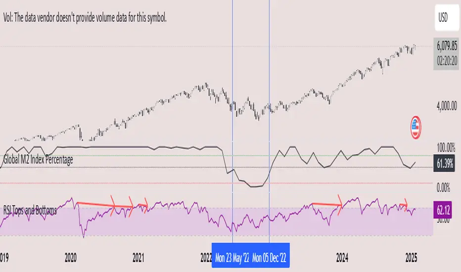
Mean Reversion Pro Strategy [tradeviZion]Mean Reversion Pro Strategy : User Guide
A mean reversion trading strategy for daily timeframe trading.
Introduction
Mean Reversion Pro Strategy is a technical trading system that operates on the daily timeframe. The strategy uses a dual Simple Moving Average (SMA) system combined with price range analysis to identify potential trading opportunities. It can be used on major indices and other markets with sufficient liquidity.
The strategy includes:
Trading System
Fast SMA for entry/exit points (5, 10, 15, 20 periods)
Slow SMA for trend reference (100, 200 periods)
Price range analysis (20% threshold)
Position management rules
Visual Elements
Gradient color indicators
Three themes (Dark/Light/Custom)
ATR-based visuals
Signal zones
Status Table
Current position information
Basic performance metrics
Strategy parameters
Optional messages
📊 Strategy Settings
Main Settings
Trading Mode
Options: Long Only, Short Only, Both
Default: Long Only
Position Size: 10% of equity
Starting Capital: $20,000
Moving Averages
Fast SMA: 5, 10, 15, or 20 periods
Slow SMA: 100 or 200 periods
Default: Fast=5, Slow=100
🎯 Entry and Exit Rules
Long Entry Conditions
All conditions must be met:
Price below Fast SMA
Price below 20% of current bar's range
Price above Slow SMA
No existing position
Short Entry Conditions
All conditions must be met:
Price above Fast SMA
Price above 80% of current bar's range
Price below Slow SMA
No existing position
Exit Rules
Long Positions
Exit when price crosses above Fast SMA
No fixed take-profit levels
No stop-loss (mean reversion approach)
Short Positions
Exit when price crosses below Fast SMA
No fixed take-profit levels
No stop-loss (mean reversion approach)
💼 Risk Management
Position Sizing
Default: 10% of equity per trade
Initial capital: $20,000
Commission: 0.01%
Slippage: 2 points
Maximum one position at a time
Risk Control
Use daily timeframe only
Avoid trading during major news events
Consider market conditions
Monitor overall exposure
📊 Performance Dashboard
The strategy includes a comprehensive status table displaying:
Strategy Parameters
Current SMA settings
Trading direction
Fast/Slow SMA ratio
Current Status
Active position (Flat/Long/Short)
Current price with color coding
Position status indicators
Performance Metrics
Net Profit (USD and %)
Win Rate with color grading
Profit Factor with thresholds
Maximum Drawdown percentage
Average Trade value
📱 Alert Settings
Entry Alerts
Long Entry (Buy Signal)
Short Entry (Sell Signal)
Exit Alerts
Long Exit (Take Profit)
Short Exit (Take Profit)
Alert Message Format
Strategy name
Signal type and direction
Current price
Fast SMA value
Slow SMA value
💡 Usage Tips
Consider starting with Long Only mode
Begin with default settings
Keep track of your trades
Review results regularly
Adjust settings as needed
Follow your trading plan
⚠️ Disclaimer
This strategy is for educational and informational purposes only. It is not financial advice. Always:
Conduct your own research
Test thoroughly before live trading
Use proper risk management
Consider your trading goals
Monitor market conditions
Never risk more than you can afford to lose
📋 Release Notes
14 January 2025
Added New Fast & Slow SMA Options:
Fibonacci-based periods: 8, 13, 21, 144, 233, 377
Additional period: 50
Complete Fast SMA options now: 5, 8, 10, 13, 15, 20, 21, 34, 50
Complete Slow SMA options now: 100, 144, 200, 233, 377
Bug Fixes:
Fixed Maximum Drawdown calculation in the performance table
Now using strategy.max_drawdown_percent for accurate DD reporting
Previous version showed incorrect DD values
Performance metrics now accurately reflect trading results
Performance Note:
Strategy tested with Fast/Slow SMA 13/377
Test conducted with 10% equity risk allocation
Daily Timeframe
For Beginners - How to Modify SMA Levels:
Find this line in the code:
fastLength = input.int(title="Fast SMA Length", defval=5, options= )
To add a new Fast SMA period: Add the number to the options list, e.g.,
To remove a Fast SMA period: Remove the number from the options list
For Slow SMA, find:
slowLength = input.int(title="Slow SMA Length", defval=100, options= )
Modify the options list the same way
⚠️ Note: Keep the periods that make sense for your trading timeframe
💡 Tip: Test any new combinations thoroughly before live trading
"Trade with Discipline, Manage Risk, Stay Consistent" - tradeviZion

All Harmonic Patterns [theEccentricTrader]█ OVERVIEW
This indicator automatically draws and sends alerts for all of the harmonic patterns in my public library as they occur. The patterns included are as follows:
• Bearish 5-0
• Bullish 5-0
• Bearish ABCD
• Bullish ABCD
• Bearish Alternate Bat
• Bullish Alternate Bat
• Bearish Bat
• Bullish Bat
• Bearish Butterfly
• Bullish Butterfly
• Bearish Cassiopeia A
• Bullish Cassiopeia A
• Bearish Cassiopeia B
• Bullish Cassiopeia B
• Bearish Cassiopeia C
• Bullish Cassiopeia C
• Bearish Crab
• Bullish Crab
• Bearish Deep Crab
• Bullish Deep Crab
• Bearish Cypher
• Bullish Cypher
• Bearish Gartley
• Bullish Gartley
• Bearish Shark
• Bullish Shark
• Bearish Three-Drive
• Bullish Three-Drive
█ CONCEPTS
Green and Red Candles
• A green candle is one that closes with a close price equal to or above the price it opened.
• A red candle is one that closes with a close price that is lower than the price it opened.
Swing Highs and Swing Lows
• A swing high is a green candle or series of consecutive green candles followed by a single red candle to complete the swing and form the peak.
• A swing low is a red candle or series of consecutive red candles followed by a single green candle to complete the swing and form the trough.
Peak and Trough Prices
• The peak price of a complete swing high is the high price of either the red candle that completes the swing high or the high price of the preceding green candle, depending on which is higher.
• The trough price of a complete swing low is the low price of either the green candle that completes the swing low or the low price of the preceding red candle, depending on which is lower.
Historic Peaks and Troughs
The current, or most recent, peak and trough occurrences are referred to as occurrence zero. Previous peak and trough occurrences are referred to as historic and ordered numerically from right to left, with the most recent historic peak and trough occurrences being occurrence one.
Upper Trends
• A return line uptrend is formed when the current peak price is higher than the preceding peak price.
• A downtrend is formed when the current peak price is lower than the preceding peak price.
• A double-top is formed when the current peak price is equal to the preceding peak price.
Lower Trends
• An uptrend is formed when the current trough price is higher than the preceding trough price.
• A return line downtrend is formed when the current trough price is lower than the preceding trough price.
• A double-bottom is formed when the current trough price is equal to the preceding trough price.
Range
The range is simply the difference between the current peak and current trough prices, generally expressed in terms of points or pips.
Wave Cycles
A wave cycle is here defined as a complete two-part move between a swing high and a swing low, or a swing low and a swing high. The first swing high or swing low will set the course for the sequence of wave cycles that follow; for example a chart that begins with a swing low will form its first complete wave cycle upon the formation of the first complete swing high and vice versa.
Figure 1.
Retracement and Extension Ratios
Retracement and extension ratios are calculated by dividing the current range by the preceding range and multiplying the answer by 100. Retracement ratios are those that are equal to or below 100% of the preceding range and extension ratios are those that are above 100% of the preceding range.
Fibonacci Retracement and Extension Ratios
The Fibonacci sequence is a series of numbers in which each number is the sum of the two preceding numbers, starting with 0 and 1. For example 0 + 1 = 1, 1 + 1 = 2, 1 + 2 = 3, and so on. Ultimately, we could go on forever but the first few numbers in the sequence are as follows: 0 , 1, 1, 2, 3, 5, 8, 13, 21, 34, 55, 89, 144.
The extension ratios are calculated by dividing each number in the sequence by the number preceding it. For example 0/1 = 0, 1/1 = 1, 2/1 = 2, 3/2 = 1.5, 5/3 = 1.6666..., 8/5 = 1.6, 13/8 = 1.625, 21/13 = 1.6153..., 34/21 = 1.6190..., 55/34 = 1.6176..., 89/55 = 1.6181..., 144/89 = 1.6179..., and so on. The retracement ratios are calculated by inverting this process and dividing each number in the sequence by the number proceeding it. For example 0/1 = 0, 1/1 = 1, 1/2 = 0.5, 2/3 = 0.666..., 3/5 = 0.6, 5/8 = 0.625, 8/13 = 0.6153..., 13/21 = 0.6190..., 21/34 = 0.6176..., 34/55 = 0.6181..., 55/89 = 0.6179..., 89/144 = 0.6180..., and so on.
Fibonacci ranges are typically drawn from left to right, with retracement levels representing ratios inside of the current range and extension levels representing ratios extended outside of the current range. If the current wave cycle ends on a swing low, the Fibonacci range is drawn from peak to trough. If the current wave cycle ends on a swing high the Fibonacci range is drawn from trough to peak.
Measurement Tolerances
Tolerance refers to the allowable variation or deviation from a specific value or dimension. It is the range within which a particular measurement is considered to be acceptable or accurate. I have applied this concept in my pattern detection logic and have set default tolerances where applicable, as perfect patterns are, needless to say, very rare.
Chart Patterns
Generally speaking price charts are nothing more than a series of swing highs and swing lows. When demand outweighs supply over a period of time prices swing higher and when supply outweighs demand over a period of time prices swing lower. These swing highs and swing lows can form patterns that offer insight into the prevailing supply and demand dynamics at play at the relevant moment in time.
‘Let us assume… that you the reader, are not a member of that mysterious inner circle known to the boardrooms as “the insiders”… But it is fairly certain that there are not nearly so many “insiders” as amateur trader supposes and… It is even more certain that insiders can be wrong… Any success they have, however, can be accomplished only by buying and selling… hey can do neither without altering the delicate poise of supply and demand that governs prices. Whatever they do is sooner or later reflected on the charts where you… can detect it. Or detect, at least, the way in which the supply-demand equation is being affected… So, you do not need to be an insider to ride with them frequently… prices move in trends. Some of those trends are straight, some are curved; some are brief and some are long and continued… produced in a series of action and reaction waves of great uniformity. Sooner or later, these trends change direction; they may reverse (as from up to down), or they may be interrupted by some sort of sideways movement and then, after a time, proceed again in their former direction… when a price trend is in the process of reversal… a characteristic area or pattern takes shape on the chart, which becomes recognisable as a reversal formation… Needless to say, the first and most important task of the technical chart analyst is to learn to know the important reversal formations and to judge what they may signify in terms of trading opportunities’ (Edwards & Magee, 1948).
This is as true today as it was when Edwards and Magee were writing in the first half of the last Century, study your patterns and make judgements for yourself about what their implications truly are on the markets and timeframes you are interested in trading.
Over the years, traders have come to discover a multitude of chart and candlestick patterns that are supposed to pertain information on future price movements. However, it is never so clear cut in practice and patterns that where once considered to be reversal patterns are now considered to be continuation patterns and vice versa. Bullish patterns can have bearish implications and bearish patterns can have bullish implications. As such, I would highly encourage you to do your own backtesting.
There is no denying that chart patterns exist, but their implications will vary from market to market and timeframe to timeframe. So it is down to you as an individual to study them and make decisions about how they may be used in a strategic sense.
Harmonic Patterns
The concept of harmonic patterns in trading was first introduced by H.M. Gartley in his book "Profits in the Stock Market", published in 1935. Gartley observed that markets have a tendency to move in repetitive patterns, and he identified several specific patterns that he believed could be used to predict future price movements. The bullish and bearish Gartley patterns are the oldest recognized harmonic patterns in trading and all the other harmonic patterns are modifications of the original Gartley patterns. Gartley patterns are fundamentally composed of 5 points, or 4 waves.
Since then, many other traders and analysts have built upon Gartley's work and developed their own variations of harmonic patterns. One such contributor is Larry Pesavento, who developed his own methods for measuring harmonic patterns using Fibonacci ratios. Pesavento has written several books on the subject of harmonic patterns and Fibonacci ratios in trading. Another notable contributor to harmonic patterns is Scott Carney, who developed his own approach to harmonic trading in the late 1990s and also popularised the use of Fibonacci ratios to measure harmonic patterns. Carney expanded on Gartley's work and also introduced several new harmonic patterns, such as the Shark pattern and the 5-0 pattern.
█ INPUTS
• Change pattern and label colours
• Show or hide patterns individually
• Adjust pattern tolerances
• Set or remove alerts for individual patterns
█ NOTES
You can test the patterns with your own strategies manually by applying the indicator to your chart while in bar replay mode and playing through the history. You could also automate this process with PineScript by using the conditions from my swing and pattern libraries as entry conditions in the strategy tester or your own custom made strategy screener.
█ LIMITATIONS
All green and red candle calculations are based on differences between open and close prices, as such I have made no attempt to account for green candles that gap lower and close below the close price of the preceding candle, or red candles that gap higher and close above the close price of the preceding candle. This may cause some unexpected behaviour on some markets and timeframes. I can only recommend using 24-hour markets, if and where possible, as there are far fewer gaps and, generally, more data to work with.
█ SOURCES
Edwards, R., & Magee, J. (1948) Technical Analysis of Stock Trends (10th edn). Reprint, Boca Raton, Florida: Taylor and Francis Group, CRC Press: 2013.
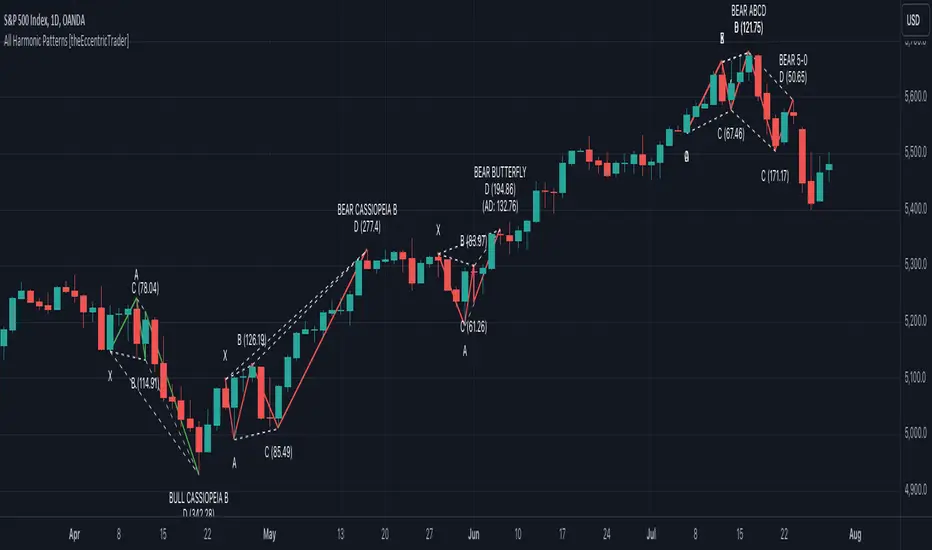
Phaser [QuantVue]The Phaser indicator is a tool to help identify inflection points by looking at price relative to past prices across multiple timeframes and assets.
Phase 1 looks for the price to be higher or lower than the closing price of the bar 4 bars earlier and is complete when 9 consecutive bars meet this criterion.
A completed Phase 1 is considered perfect when the highs (bearish) or lows (bullish) have been exceeded from bars 6 and 7 of the phase.
A bullish setup requires 9 consecutive closes less than the close 4 bars earlier.
A bearish setup requires 9 consecutive closes greater than the close 4 bars earlier.
Phase 2 begins once Phase 1 has been completed. Phase 2 compares the current price to the high or low of two bars earlier.
Unlike Phase 1, Phase 2 does not require the count to be consecutive.
Phase 2 is considered complete when 13 candles have met the criteria.
An important aspect to Phase 2 is the relationship between bar 13 and bar 8.
To ensure the end of Phase 2 is in line with the existing trend, the high or low of bar 13 is compared to the close of bar 8.
A bullish imperfect 13 occurs when the current price is less than the low of 2 bars earlier, but the current low is greater than the close of bar 8 in Phase 2.
A bearish imperfect 13 occurs when the current price is greater than the high of 2 bars earlier, but the current high is less than the close of bar 8 in Phase 2.
Phase 2 does not need to go until it is complete. A Phase 2 can be canceled if the price closes above or below the highest or lowest price from Phase 1.
Settings
3 Tickers
3 Timeframes
Show Phase 1
Show Phase 2
User-selected colors
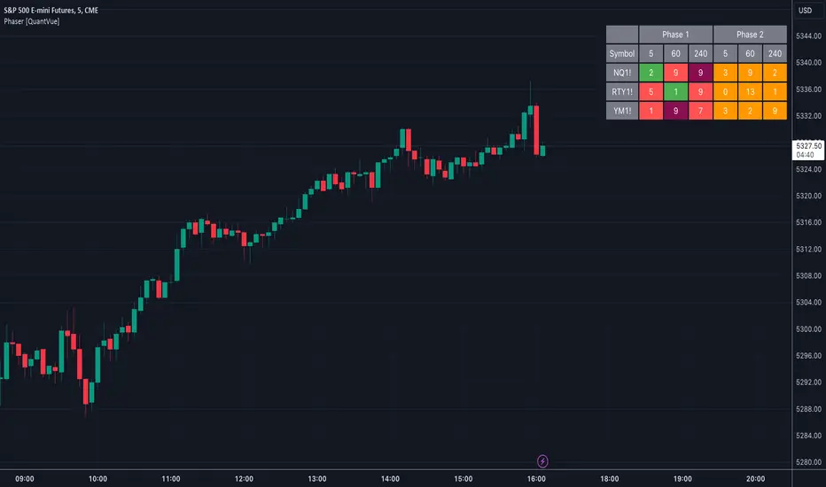
Bearish Cassiopeia C Harmonic Patterns [theEccentricTrader]█ OVERVIEW
This indicator automatically detects and draws bearish Cassiopeia C harmonic patterns and price projections derived from the ranges that constitute the patterns.
Cassiopeia A, B and C harmonic patterns are patterns that I created/discovered myself. They are all inspired by the Cassiopeia constellation and each one is based on different rotations of the constellation as it moves through the sky. The range ratios are also based on the constellation's right ascension and declination listed on Wikipedia:
Right ascension 22h 57m 04.5897s–03h 41m 14.0997s
Declination 77.6923447°–48.6632690°
en.wikipedia.org
I actually developed this idea quite a while ago now but have not felt audacious enough to introduce a new harmonic pattern, let alone 3 at the same time! But I have since been able to run backtests on tick data going back to 2002 across a variety of market and timeframe combinations and have learned that the Cassiopeia patterns can certainly hold their own against the currently known harmonic patterns.
I would also point out that the Cassiopeia constellation does actually look like a harmonic pattern and the Cassiopeia A star is literally the 'strongest source of radio emission in the sky beyond the solar system', so its arguably more of a real harmonic phenomenon than the current patterns.
www.britannica.com
chandra.si.edu
█ CONCEPTS
Green and Red Candles
• A green candle is one that closes with a close price equal to or above the price it opened.
• A red candle is one that closes with a close price that is lower than the price it opened.
Swing Highs and Swing Lows
• A swing high is a green candle or series of consecutive green candles followed by a single red candle to complete the swing and form the peak.
• A swing low is a red candle or series of consecutive red candles followed by a single green candle to complete the swing and form the trough.
Peak and Trough Prices (Basic)
• The peak price of a complete swing high is the high price of either the red candle that completes the swing high or the high price of the preceding green candle, depending on which is higher.
• The trough price of a complete swing low is the low price of either the green candle that completes the swing low or the low price of the preceding red candle, depending on which is lower.
Historic Peaks and Troughs
The current, or most recent, peak and trough occurrences are referred to as occurrence zero. Previous peak and trough occurrences are referred to as historic and ordered numerically from right to left, with the most recent historic peak and trough occurrences being occurrence one.
Range
The range is simply the difference between the current peak and current trough prices, generally expressed in terms of points or pips.
Upper Trends
• A return line uptrend is formed when the current peak price is higher than the preceding peak price.
• A downtrend is formed when the current peak price is lower than the preceding peak price.
• A double-top is formed when the current peak price is equal to the preceding peak price.
Lower Trends
• An uptrend is formed when the current trough price is higher than the preceding trough price.
• A return line downtrend is formed when the current trough price is lower than the preceding trough price.
• A double-bottom is formed when the current trough price is equal to the preceding trough price.
Muti-Part Upper and Lower Trends
• A multi-part return line uptrend begins with the formation of a new return line uptrend and continues until a new downtrend ends the trend.
• A multi-part downtrend begins with the formation of a new downtrend and continues until a new return line uptrend ends the trend.
• A multi-part uptrend begins with the formation of a new uptrend and continues until a new return line downtrend ends the trend.
• A multi-part return line downtrend begins with the formation of a new return line downtrend and continues until a new uptrend ends the trend.
Double Trends
• A double uptrend is formed when the current trough price is higher than the preceding trough price and the current peak price is higher than the preceding peak price.
• A double downtrend is formed when the current peak price is lower than the preceding peak price and the current trough price is lower than the preceding trough price.
Muti-Part Double Trends
• A multi-part double uptrend begins with the formation of a new uptrend that proceeds a new return line uptrend, and continues until a new downtrend or return line downtrend ends the trend.
• A multi-part double downtrend begins with the formation of a new downtrend that proceeds a new return line downtrend, and continues until a new uptrend or return line uptrend ends the trend.
Wave Cycles
A wave cycle is here defined as a complete two-part move between a swing high and a swing low, or a swing low and a swing high. The first swing high or swing low will set the course for the sequence of wave cycles that follow; for example a chart that begins with a swing low will form its first complete wave cycle upon the formation of the first complete swing high and vice versa.
Figure 1.
Retracement and Extension Ratios
Retracement and extension ratios are calculated by dividing the current range by the preceding range and multiplying the answer by 100. Retracement ratios are those that are equal to or below 100% of the preceding range and extension ratios are those that are above 100% of the preceding range.
Fibonacci Retracement and Extension Ratios
The Fibonacci sequence is a series of numbers in which each number is the sum of the two preceding numbers, starting with 0 and 1. For example 0 + 1 = 1, 1 + 1 = 2, 1 + 2 = 3, and so on. Ultimately, we could go on forever but the first few numbers in the sequence are as follows: 0 , 1, 1, 2, 3, 5, 8, 13, 21, 34, 55, 89, 144.
The extension ratios are calculated by dividing each number in the sequence by the number preceding it. For example 0/1 = 0, 1/1 = 1, 2/1 = 2, 3/2 = 1.5, 5/3 = 1.6666..., 8/5 = 1.6, 13/8 = 1.625, 21/13 = 1.6153..., 34/21 = 1.6190..., 55/34 = 1.6176..., 89/55 = 1.6181..., 144/89 = 1.6179..., and so on. The retracement ratios are calculated by inverting this process and dividing each number in the sequence by the number proceeding it. For example 0/1 = 0, 1/1 = 1, 1/2 = 0.5, 2/3 = 0.666..., 3/5 = 0.6, 5/8 = 0.625, 8/13 = 0.6153..., 13/21 = 0.6190..., 21/34 = 0.6176..., 34/55 = 0.6181..., 55/89 = 0.6179..., 89/144 = 0.6180..., and so on.
1.618 is considered to be the 'golden ratio', found in many natural phenomena such as the growth of seashells and the branching of trees. Some now speculate the universe oscillates at a frequency of 0,618 Hz, which could help to explain such phenomena, but this theory has yet to be proven.
Traders and analysts use Fibonacci retracement and extension indicators, consisting of horizontal lines representing different Fibonacci ratios, for identifying potential levels of support and resistance. Fibonacci ranges are typically drawn from left to right, with retracement levels representing ratios inside of the current range and extension levels representing ratios extended outside of the current range. If the current wave cycle ends on a swing low, the Fibonacci range is drawn from peak to trough. If the current wave cycle ends on a swing high the Fibonacci range is drawn from trough to peak.
Harmonic Patterns
The concept of harmonic patterns in trading was first introduced by H.M. Gartley in his book "Profits in the Stock Market", published in 1935. Gartley observed that markets have a tendency to move in repetitive patterns, and he identified several specific patterns that he believed could be used to predict future price movements.
Since then, many other traders and analysts have built upon Gartley's work and developed their own variations of harmonic patterns. One such contributor is Larry Pesavento, who developed his own methods for measuring harmonic patterns using Fibonacci ratios. Pesavento has written several books on the subject of harmonic patterns and Fibonacci ratios in trading. Another notable contributor to harmonic patterns is Scott Carney, who developed his own approach to harmonic trading in the late 1990s and also popularised the use of Fibonacci ratios to measure harmonic patterns. Carney expanded on Gartley's work and also introduced several new harmonic patterns, such as the Shark pattern and the 5-0 pattern.
The bullish and bearish Gartley patterns are the oldest recognized harmonic patterns in trading and all the other harmonic patterns are ultimately modifications of the original Gartley patterns. Gartley patterns are fundamentally composed of 5 points, or 4 waves.
Bullish and Bearish Cassiopeia C Harmonic Patterns
• Bullish Cassiopeia C patterns are fundamentally composed of three troughs and two peaks. The second peak being higher than the first peak. And the third trough being lower than both the first and second troughs, while the second trough is higher than the first.
• Bearish Cassiopeia C patterns are fundamentally composed of three peaks and two troughs. The second trough being lower than the first trough. And the third peak being higher than both the first and second peaks, while the second peak is lower than the first.
The ratio measurements I use to detect the patterns are as follows:
• Wave 1 of the pattern, generally referred to as XA, has no specific ratio requirements.
• Wave 2 of the pattern, generally referred to as AB, should retrace by at least 11.34%, but no further than 22.31% of the range set by wave 1.
• Wave 3 of the pattern, generally referred to as BC, should extend by at least 225.7%, but no further than 341% of the range set by wave 2.
• Wave 4 of the pattern, generally referred to as CD, should retrace by at least 77.69%, but no further than 88.66% of the range set by wave 3.
Measurement Tolerances
In general, tolerance in measurements refers to the allowable variation or deviation from a specific value or dimension. It is the range within which a particular measurement is considered to be acceptable or accurate. In this script I have applied this concept to the measurement of harmonic pattern ratios to increase to the frequency of pattern occurrences.
For example, the AB measurement of Gartley patterns is generally set at around 61.8%, but with such specificity in the measuring requirements the patterns are very rare. We can increase the frequency of pattern occurrences by setting a tolerance. A tolerance of 10% to both downside and upside, which is the default setting for all tolerances, means we would have a tolerable measurement range between 51.8-71.8%, thus increasing the frequency of occurrence.
█ FEATURES
Inputs
• AB Lower Tolerance
• AB Upper Tolerance
• BC Lower Tolerance
• BC Upper Tolerance
• CD Lower Tolerance
• CD Upper Tolerance
• Pattern Color
• Label Color
• Show Projections
• Extend Current Projection Lines
Alerts
Users can set alerts for when the patterns occur.
█ LIMITATIONS
All green and red candle calculations are based on differences between open and close prices, as such I have made no attempt to account for green candles that gap lower and close below the close price of the preceding candle, or red candles that gap higher and close above the close price of the preceding candle. This may cause some unexpected behaviour on some markets and timeframes. I can only recommend using 24-hour markets, if and where possible, as there are far fewer gaps and, generally, more data to work with.
█ NOTES
I know a few people have been requesting a single indicator that contains all my patterns and I definitely hear you on that one. However, I have been very busy working on other projects while trying to trade and be a human at the same time. For now I am going to maintain my original approach of releasing each pattern individually so as to maintain consistency. But I am now also working on getting my some of my libraries ready for public release and in doing so I will finally be able to fit all patterns into one script. I will also be giving my scripts some TLC by making them cleaner once I have the libraries up and running. Please bear with me in the meantime, this may take a while. Cheers!

Bullish Cassiopeia C Harmonic Patterns [theEccentricTrader]█ OVERVIEW
This indicator automatically detects and draws bullish Cassiopeia C harmonic patterns and price projections derived from the ranges that constitute the patterns.
Cassiopeia A, B and C harmonic patterns are patterns that I created/discovered myself. They are all inspired by the Cassiopeia constellation and each one is based on different rotations of the constellation as it moves through the sky. The range ratios are also based on the constellation's right ascension and declination listed on Wikipedia:
Right ascension 22h 57m 04.5897s–03h 41m 14.0997s
Declination 77.6923447°–48.6632690°
en.wikipedia.org
I actually developed this idea quite a while ago now but have not felt audacious enough to introduce a new harmonic pattern, let alone 3 at the same time! But I have since been able to run backtests on tick data going back to 2002 across a variety of market and timeframe combinations and have learned that the Cassiopeia patterns can certainly hold their own against the currently known harmonic patterns.
I would also point out that the Cassiopeia constellation does actually look like a harmonic pattern and the Cassiopeia A star is literally the 'strongest source of radio emission in the sky beyond the solar system', so its arguably more of a real harmonic phenomenon than the current patterns.
www.britannica.com
chandra.si.edu
█ CONCEPTS
Green and Red Candles
• A green candle is one that closes with a close price equal to or above the price it opened.
• A red candle is one that closes with a close price that is lower than the price it opened.
Swing Highs and Swing Lows
• A swing high is a green candle or series of consecutive green candles followed by a single red candle to complete the swing and form the peak.
• A swing low is a red candle or series of consecutive red candles followed by a single green candle to complete the swing and form the trough.
Peak and Trough Prices (Basic)
• The peak price of a complete swing high is the high price of either the red candle that completes the swing high or the high price of the preceding green candle, depending on which is higher.
• The trough price of a complete swing low is the low price of either the green candle that completes the swing low or the low price of the preceding red candle, depending on which is lower.
Historic Peaks and Troughs
The current, or most recent, peak and trough occurrences are referred to as occurrence zero. Previous peak and trough occurrences are referred to as historic and ordered numerically from right to left, with the most recent historic peak and trough occurrences being occurrence one.
Range
The range is simply the difference between the current peak and current trough prices, generally expressed in terms of points or pips.
Upper Trends
• A return line uptrend is formed when the current peak price is higher than the preceding peak price.
• A downtrend is formed when the current peak price is lower than the preceding peak price.
• A double-top is formed when the current peak price is equal to the preceding peak price.
Lower Trends
• An uptrend is formed when the current trough price is higher than the preceding trough price.
• A return line downtrend is formed when the current trough price is lower than the preceding trough price.
• A double-bottom is formed when the current trough price is equal to the preceding trough price.
Muti-Part Upper and Lower Trends
• A multi-part return line uptrend begins with the formation of a new return line uptrend and continues until a new downtrend ends the trend.
• A multi-part downtrend begins with the formation of a new downtrend and continues until a new return line uptrend ends the trend.
• A multi-part uptrend begins with the formation of a new uptrend and continues until a new return line downtrend ends the trend.
• A multi-part return line downtrend begins with the formation of a new return line downtrend and continues until a new uptrend ends the trend.
Double Trends
• A double uptrend is formed when the current trough price is higher than the preceding trough price and the current peak price is higher than the preceding peak price.
• A double downtrend is formed when the current peak price is lower than the preceding peak price and the current trough price is lower than the preceding trough price.
Muti-Part Double Trends
• A multi-part double uptrend begins with the formation of a new uptrend that proceeds a new return line uptrend, and continues until a new downtrend or return line downtrend ends the trend.
• A multi-part double downtrend begins with the formation of a new downtrend that proceeds a new return line downtrend, and continues until a new uptrend or return line uptrend ends the trend.
Wave Cycles
A wave cycle is here defined as a complete two-part move between a swing high and a swing low, or a swing low and a swing high. The first swing high or swing low will set the course for the sequence of wave cycles that follow; for example a chart that begins with a swing low will form its first complete wave cycle upon the formation of the first complete swing high and vice versa.
Figure 1.
Retracement and Extension Ratios
Retracement and extension ratios are calculated by dividing the current range by the preceding range and multiplying the answer by 100. Retracement ratios are those that are equal to or below 100% of the preceding range and extension ratios are those that are above 100% of the preceding range.
Fibonacci Retracement and Extension Ratios
The Fibonacci sequence is a series of numbers in which each number is the sum of the two preceding numbers, starting with 0 and 1. For example 0 + 1 = 1, 1 + 1 = 2, 1 + 2 = 3, and so on. Ultimately, we could go on forever but the first few numbers in the sequence are as follows: 0 , 1, 1, 2, 3, 5, 8, 13, 21, 34, 55, 89, 144.
The extension ratios are calculated by dividing each number in the sequence by the number preceding it. For example 0/1 = 0, 1/1 = 1, 2/1 = 2, 3/2 = 1.5, 5/3 = 1.6666..., 8/5 = 1.6, 13/8 = 1.625, 21/13 = 1.6153..., 34/21 = 1.6190..., 55/34 = 1.6176..., 89/55 = 1.6181..., 144/89 = 1.6179..., and so on. The retracement ratios are calculated by inverting this process and dividing each number in the sequence by the number proceeding it. For example 0/1 = 0, 1/1 = 1, 1/2 = 0.5, 2/3 = 0.666..., 3/5 = 0.6, 5/8 = 0.625, 8/13 = 0.6153..., 13/21 = 0.6190..., 21/34 = 0.6176..., 34/55 = 0.6181..., 55/89 = 0.6179..., 89/144 = 0.6180..., and so on.
1.618 is considered to be the 'golden ratio', found in many natural phenomena such as the growth of seashells and the branching of trees. Some now speculate the universe oscillates at a frequency of 0,618 Hz, which could help to explain such phenomena, but this theory has yet to be proven.
Traders and analysts use Fibonacci retracement and extension indicators, consisting of horizontal lines representing different Fibonacci ratios, for identifying potential levels of support and resistance. Fibonacci ranges are typically drawn from left to right, with retracement levels representing ratios inside of the current range and extension levels representing ratios extended outside of the current range. If the current wave cycle ends on a swing low, the Fibonacci range is drawn from peak to trough. If the current wave cycle ends on a swing high the Fibonacci range is drawn from trough to peak.
Harmonic Patterns
The concept of harmonic patterns in trading was first introduced by H.M. Gartley in his book "Profits in the Stock Market", published in 1935. Gartley observed that markets have a tendency to move in repetitive patterns, and he identified several specific patterns that he believed could be used to predict future price movements.
Since then, many other traders and analysts have built upon Gartley's work and developed their own variations of harmonic patterns. One such contributor is Larry Pesavento, who developed his own methods for measuring harmonic patterns using Fibonacci ratios. Pesavento has written several books on the subject of harmonic patterns and Fibonacci ratios in trading. Another notable contributor to harmonic patterns is Scott Carney, who developed his own approach to harmonic trading in the late 1990s and also popularised the use of Fibonacci ratios to measure harmonic patterns. Carney expanded on Gartley's work and also introduced several new harmonic patterns, such as the Shark pattern and the 5-0 pattern.
The bullish and bearish Gartley patterns are the oldest recognized harmonic patterns in trading and all the other harmonic patterns are ultimately modifications of the original Gartley patterns. Gartley patterns are fundamentally composed of 5 points, or 4 waves.
Bullish and Bearish Cassiopeia C Harmonic Patterns
• Bullish Cassiopeia C patterns are fundamentally composed of three troughs and two peaks. The second peak being higher than the first peak. And the third trough being lower than both the first and second troughs, while the second trough is higher than the first.
• Bearish Cassiopeia C patterns are fundamentally composed of three peaks and two troughs. The second trough being lower than the first trough. And the third peak being higher than both the first and second peaks, while the second peak is lower than the first.
The ratio measurements I use to detect the patterns are as follows:
• Wave 1 of the pattern, generally referred to as XA, has no specific ratio requirements.
• Wave 2 of the pattern, generally referred to as AB, should retrace by at least 11.34%, but no further than 22.31% of the range set by wave 1.
• Wave 3 of the pattern, generally referred to as BC, should extend by at least 225.7%, but no further than 341% of the range set by wave 2.
• Wave 4 of the pattern, generally referred to as CD, should retrace by at least 77.69%, but no further than 88.66% of the range set by wave 3.
Measurement Tolerances
In general, tolerance in measurements refers to the allowable variation or deviation from a specific value or dimension. It is the range within which a particular measurement is considered to be acceptable or accurate. In this script I have applied this concept to the measurement of harmonic pattern ratios to increase to the frequency of pattern occurrences.
For example, the AB measurement of Gartley patterns is generally set at around 61.8%, but with such specificity in the measuring requirements the patterns are very rare. We can increase the frequency of pattern occurrences by setting a tolerance. A tolerance of 10% to both downside and upside, which is the default setting for all tolerances, means we would have a tolerable measurement range between 51.8-71.8%, thus increasing the frequency of occurrence.
█ FEATURES
Inputs
• AB Lower Tolerance
• AB Upper Tolerance
• BC Lower Tolerance
• BC Upper Tolerance
• CD Lower Tolerance
• CD Upper Tolerance
• Pattern Color
• Label Color
• Show Projections
• Extend Current Projection Lines
Alerts
Users can set alerts for when the patterns occur.
█ LIMITATIONS
All green and red candle calculations are based on differences between open and close prices, as such I have made no attempt to account for green candles that gap lower and close below the close price of the preceding candle, or red candles that gap higher and close above the close price of the preceding candle. This may cause some unexpected behaviour on some markets and timeframes. I can only recommend using 24-hour markets, if and where possible, as there are far fewer gaps and, generally, more data to work with.
█ NOTES
I know a few people have been requesting a single indicator that contains all my patterns and I definitely hear you on that one. However, I have been very busy working on other projects while trying to trade and be a human at the same time. For now I am going to maintain my original approach of releasing each pattern individually so as to maintain consistency. But I am now also working on getting my some of my libraries ready for public release and in doing so I will finally be able to fit all patterns into one script. I will also be giving my scripts some TLC by making them cleaner once I have the libraries up and running. Please bear with me in the meantime, this may take a while. Cheers!

Bearish Cassiopeia B Harmonic Patterns [theEccentricTrader]█ OVERVIEW
This indicator automatically detects and draws bearish Cassiopeia B harmonic patterns and price projections derived from the ranges that constitute the patterns.
Cassiopeia A, B and C harmonic patterns are patterns that I created/discovered myself. They are all inspired by the Cassiopeia constellation and each one is based on different rotations of the constellation as it moves through the sky. The range ratios are also based on the constellation's right ascension and declination listed on Wikipedia:
Right ascension 22h 57m 04.5897s–03h 41m 14.0997s
Declination 77.6923447°–48.6632690°
en.wikipedia.org
I actually developed this idea quite a while ago now but have not felt audacious enough to introduce a new harmonic pattern, let alone 3 at the same time! But I have since been able to run backtests on tick data going back to 2002 across a variety of market and timeframe combinations and have learned that the Cassiopeia patterns can certainly hold their own against the currently known harmonic patterns.
I would also point out that the Cassiopeia constellation does actually look like a harmonic pattern and the Cassiopeia A star is literally the 'strongest source of radio emission in the sky beyond the solar system', so its arguably more of a real harmonic phenomenon than the current patterns.
www.britannica.com
chandra.si.edu
█ CONCEPTS
Green and Red Candles
• A green candle is one that closes with a close price equal to or above the price it opened.
• A red candle is one that closes with a close price that is lower than the price it opened.
Swing Highs and Swing Lows
• A swing high is a green candle or series of consecutive green candles followed by a single red candle to complete the swing and form the peak.
• A swing low is a red candle or series of consecutive red candles followed by a single green candle to complete the swing and form the trough.
Peak and Trough Prices (Basic)
• The peak price of a complete swing high is the high price of either the red candle that completes the swing high or the high price of the preceding green candle, depending on which is higher.
• The trough price of a complete swing low is the low price of either the green candle that completes the swing low or the low price of the preceding red candle, depending on which is lower.
Historic Peaks and Troughs
The current, or most recent, peak and trough occurrences are referred to as occurrence zero. Previous peak and trough occurrences are referred to as historic and ordered numerically from right to left, with the most recent historic peak and trough occurrences being occurrence one.
Range
The range is simply the difference between the current peak and current trough prices, generally expressed in terms of points or pips.
Upper Trends
• A return line uptrend is formed when the current peak price is higher than the preceding peak price.
• A downtrend is formed when the current peak price is lower than the preceding peak price.
• A double-top is formed when the current peak price is equal to the preceding peak price.
Lower Trends
• An uptrend is formed when the current trough price is higher than the preceding trough price.
• A return line downtrend is formed when the current trough price is lower than the preceding trough price.
• A double-bottom is formed when the current trough price is equal to the preceding trough price.
Muti-Part Upper and Lower Trends
• A multi-part return line uptrend begins with the formation of a new return line uptrend and continues until a new downtrend ends the trend.
• A multi-part downtrend begins with the formation of a new downtrend and continues until a new return line uptrend ends the trend.
• A multi-part uptrend begins with the formation of a new uptrend and continues until a new return line downtrend ends the trend.
• A multi-part return line downtrend begins with the formation of a new return line downtrend and continues until a new uptrend ends the trend.
Double Trends
• A double uptrend is formed when the current trough price is higher than the preceding trough price and the current peak price is higher than the preceding peak price.
• A double downtrend is formed when the current peak price is lower than the preceding peak price and the current trough price is lower than the preceding trough price.
Muti-Part Double Trends
• A multi-part double uptrend begins with the formation of a new uptrend that proceeds a new return line uptrend, and continues until a new downtrend or return line downtrend ends the trend.
• A multi-part double downtrend begins with the formation of a new downtrend that proceeds a new return line downtrend, and continues until a new uptrend or return line uptrend ends the trend.
Wave Cycles
A wave cycle is here defined as a complete two-part move between a swing high and a swing low, or a swing low and a swing high. The first swing high or swing low will set the course for the sequence of wave cycles that follow; for example a chart that begins with a swing low will form its first complete wave cycle upon the formation of the first complete swing high and vice versa.
Figure 1.
Retracement and Extension Ratios
Retracement and extension ratios are calculated by dividing the current range by the preceding range and multiplying the answer by 100. Retracement ratios are those that are equal to or below 100% of the preceding range and extension ratios are those that are above 100% of the preceding range.
Fibonacci Retracement and Extension Ratios
The Fibonacci sequence is a series of numbers in which each number is the sum of the two preceding numbers, starting with 0 and 1. For example 0 + 1 = 1, 1 + 1 = 2, 1 + 2 = 3, and so on. Ultimately, we could go on forever but the first few numbers in the sequence are as follows: 0 , 1, 1, 2, 3, 5, 8, 13, 21, 34, 55, 89, 144.
The extension ratios are calculated by dividing each number in the sequence by the number preceding it. For example 0/1 = 0, 1/1 = 1, 2/1 = 2, 3/2 = 1.5, 5/3 = 1.6666..., 8/5 = 1.6, 13/8 = 1.625, 21/13 = 1.6153..., 34/21 = 1.6190..., 55/34 = 1.6176..., 89/55 = 1.6181..., 144/89 = 1.6179..., and so on. The retracement ratios are calculated by inverting this process and dividing each number in the sequence by the number proceeding it. For example 0/1 = 0, 1/1 = 1, 1/2 = 0.5, 2/3 = 0.666..., 3/5 = 0.6, 5/8 = 0.625, 8/13 = 0.6153..., 13/21 = 0.6190..., 21/34 = 0.6176..., 34/55 = 0.6181..., 55/89 = 0.6179..., 89/144 = 0.6180..., and so on.
1.618 is considered to be the 'golden ratio', found in many natural phenomena such as the growth of seashells and the branching of trees. Some now speculate the universe oscillates at a frequency of 0,618 Hz, which could help to explain such phenomena, but this theory has yet to be proven.
Traders and analysts use Fibonacci retracement and extension indicators, consisting of horizontal lines representing different Fibonacci ratios, for identifying potential levels of support and resistance. Fibonacci ranges are typically drawn from left to right, with retracement levels representing ratios inside of the current range and extension levels representing ratios extended outside of the current range. If the current wave cycle ends on a swing low, the Fibonacci range is drawn from peak to trough. If the current wave cycle ends on a swing high the Fibonacci range is drawn from trough to peak.
Harmonic Patterns
The concept of harmonic patterns in trading was first introduced by H.M. Gartley in his book "Profits in the Stock Market", published in 1935. Gartley observed that markets have a tendency to move in repetitive patterns, and he identified several specific patterns that he believed could be used to predict future price movements.
Since then, many other traders and analysts have built upon Gartley's work and developed their own variations of harmonic patterns. One such contributor is Larry Pesavento, who developed his own methods for measuring harmonic patterns using Fibonacci ratios. Pesavento has written several books on the subject of harmonic patterns and Fibonacci ratios in trading. Another notable contributor to harmonic patterns is Scott Carney, who developed his own approach to harmonic trading in the late 1990s and also popularised the use of Fibonacci ratios to measure harmonic patterns. Carney expanded on Gartley's work and also introduced several new harmonic patterns, such as the Shark pattern and the 5-0 pattern.
The bullish and bearish Gartley patterns are the oldest recognized harmonic patterns in trading and all the other harmonic patterns are ultimately modifications of the original Gartley patterns. Gartley patterns are fundamentally composed of 5 points, or 4 waves.
Bullish and Bearish Cassiopeia B Harmonic Patterns
• Bullish Cassiopeia B patterns are fundamentally composed of three troughs and two peaks. The second peak being lower than the first peak. And the third trough being lower than both the first and second troughs, while the second trough is also lower than the first.
• Bearish Cassiopeia B patterns are fundamentally composed of three peaks and two troughs. The second trough being higher than the first trough. And the third peak being higher than both the first and second peaks, while the second peak is also higher than the first.
The ratio measurements I use to detect the patterns are as follows:
• Wave 1 of the pattern, generally referred to as XA, has no specific ratio requirements.
• Wave 2 of the pattern, generally referred to as AB, should retrace by at least 11.34%, but no further than 22.31% of the range set by wave 1.
• Wave 3 of the pattern, generally referred to as BC, should extend by at least 225.7%, but no further than 341% of the range set by wave 2.
• Wave 4 of the pattern, generally referred to as CD, should retrace by at least 77.69%, but no further than 88.66% of the range set by wave 3.
Measurement Tolerances
In general, tolerance in measurements refers to the allowable variation or deviation from a specific value or dimension. It is the range within which a particular measurement is considered to be acceptable or accurate. In this script I have applied this concept to the measurement of harmonic pattern ratios to increase to the frequency of pattern occurrences.
For example, the AB measurement of Gartley patterns is generally set at around 61.8%, but with such specificity in the measuring requirements the patterns are very rare. We can increase the frequency of pattern occurrences by setting a tolerance. A tolerance of 10% to both downside and upside, which is the default setting for all tolerances, means we would have a tolerable measurement range between 51.8-71.8%, thus increasing the frequency of occurrence.
█ FEATURES
Inputs
• AB Lower Tolerance
• AB Upper Tolerance
• BC Lower Tolerance
• BC Upper Tolerance
• CD Lower Tolerance
• CD Upper Tolerance
• Pattern Color
• Label Color
• Show Projections
• Extend Current Projection Lines
Alerts
Users can set alerts for when the patterns occur.
█ LIMITATIONS
All green and red candle calculations are based on differences between open and close prices, as such I have made no attempt to account for green candles that gap lower and close below the close price of the preceding candle, or red candles that gap higher and close above the close price of the preceding candle. This may cause some unexpected behaviour on some markets and timeframes. I can only recommend using 24-hour markets, if and where possible, as there are far fewer gaps and, generally, more data to work with.
█ NOTES
I know a few people have been requesting a single indicator that contains all my patterns and I definitely hear you on that one. However, I have been very busy working on other projects while trying to trade and be a human at the same time. For now I am going to maintain my original approach of releasing each pattern individually so as to maintain consistency. But I am now also working on getting my some of my libraries ready for public release and in doing so I will finally be able to fit all patterns into one script. I will also be giving my scripts some TLC by making them cleaner once I have the libraries up and running. Please bear with me in the meantime, this may take a while. Cheers!

Bullish Cassiopeia B Harmonic Patterns [theEccentricTrader]█ OVERVIEW
This indicator automatically detects and draws bullish Cassiopeia B harmonic patterns and price projections derived from the ranges that constitute the patterns.
Cassiopeia A, B and C harmonic patterns are patterns that I created/discovered myself. They are all inspired by the Cassiopeia constellation and each one is based on different rotations of the constellation as it moves through the sky. The range ratios are also based on the constellation's right ascension and declination listed on Wikipedia:
Right ascension 22h 57m 04.5897s–03h 41m 14.0997s
Declination 77.6923447°–48.6632690°
en.wikipedia.org
I actually developed this idea quite a while ago now but have not felt audacious enough to introduce a new harmonic pattern, let alone 3 at the same time! But I have since been able to run backtests on tick data going back to 2002 across a variety of market and timeframe combinations and have learned that the Cassiopeia patterns can certainly hold their own against the currently known harmonic patterns.
I would also point out that the Cassiopeia constellation does actually look like a harmonic pattern and the Cassiopeia A star is literally the 'strongest source of radio emission in the sky beyond the solar system', so its arguably more of a real harmonic phenomenon than the current patterns.
www.britannica.com
chandra.si.edu
█ CONCEPTS
Green and Red Candles
• A green candle is one that closes with a close price equal to or above the price it opened.
• A red candle is one that closes with a close price that is lower than the price it opened.
Swing Highs and Swing Lows
• A swing high is a green candle or series of consecutive green candles followed by a single red candle to complete the swing and form the peak.
• A swing low is a red candle or series of consecutive red candles followed by a single green candle to complete the swing and form the trough.
Peak and Trough Prices (Basic)
• The peak price of a complete swing high is the high price of either the red candle that completes the swing high or the high price of the preceding green candle, depending on which is higher.
• The trough price of a complete swing low is the low price of either the green candle that completes the swing low or the low price of the preceding red candle, depending on which is lower.
Historic Peaks and Troughs
The current, or most recent, peak and trough occurrences are referred to as occurrence zero. Previous peak and trough occurrences are referred to as historic and ordered numerically from right to left, with the most recent historic peak and trough occurrences being occurrence one.
Range
The range is simply the difference between the current peak and current trough prices, generally expressed in terms of points or pips.
Upper Trends
• A return line uptrend is formed when the current peak price is higher than the preceding peak price.
• A downtrend is formed when the current peak price is lower than the preceding peak price.
• A double-top is formed when the current peak price is equal to the preceding peak price.
Lower Trends
• An uptrend is formed when the current trough price is higher than the preceding trough price.
• A return line downtrend is formed when the current trough price is lower than the preceding trough price.
• A double-bottom is formed when the current trough price is equal to the preceding trough price.
Muti-Part Upper and Lower Trends
• A multi-part return line uptrend begins with the formation of a new return line uptrend and continues until a new downtrend ends the trend.
• A multi-part downtrend begins with the formation of a new downtrend and continues until a new return line uptrend ends the trend.
• A multi-part uptrend begins with the formation of a new uptrend and continues until a new return line downtrend ends the trend.
• A multi-part return line downtrend begins with the formation of a new return line downtrend and continues until a new uptrend ends the trend.
Double Trends
• A double uptrend is formed when the current trough price is higher than the preceding trough price and the current peak price is higher than the preceding peak price.
• A double downtrend is formed when the current peak price is lower than the preceding peak price and the current trough price is lower than the preceding trough price.
Muti-Part Double Trends
• A multi-part double uptrend begins with the formation of a new uptrend that proceeds a new return line uptrend, and continues until a new downtrend or return line downtrend ends the trend.
• A multi-part double downtrend begins with the formation of a new downtrend that proceeds a new return line downtrend, and continues until a new uptrend or return line uptrend ends the trend.
Wave Cycles
A wave cycle is here defined as a complete two-part move between a swing high and a swing low, or a swing low and a swing high. The first swing high or swing low will set the course for the sequence of wave cycles that follow; for example a chart that begins with a swing low will form its first complete wave cycle upon the formation of the first complete swing high and vice versa.
Figure 1.
Retracement and Extension Ratios
Retracement and extension ratios are calculated by dividing the current range by the preceding range and multiplying the answer by 100. Retracement ratios are those that are equal to or below 100% of the preceding range and extension ratios are those that are above 100% of the preceding range.
Fibonacci Retracement and Extension Ratios
The Fibonacci sequence is a series of numbers in which each number is the sum of the two preceding numbers, starting with 0 and 1. For example 0 + 1 = 1, 1 + 1 = 2, 1 + 2 = 3, and so on. Ultimately, we could go on forever but the first few numbers in the sequence are as follows: 0 , 1, 1, 2, 3, 5, 8, 13, 21, 34, 55, 89, 144.
The extension ratios are calculated by dividing each number in the sequence by the number preceding it. For example 0/1 = 0, 1/1 = 1, 2/1 = 2, 3/2 = 1.5, 5/3 = 1.6666..., 8/5 = 1.6, 13/8 = 1.625, 21/13 = 1.6153..., 34/21 = 1.6190..., 55/34 = 1.6176..., 89/55 = 1.6181..., 144/89 = 1.6179..., and so on. The retracement ratios are calculated by inverting this process and dividing each number in the sequence by the number proceeding it. For example 0/1 = 0, 1/1 = 1, 1/2 = 0.5, 2/3 = 0.666..., 3/5 = 0.6, 5/8 = 0.625, 8/13 = 0.6153..., 13/21 = 0.6190..., 21/34 = 0.6176..., 34/55 = 0.6181..., 55/89 = 0.6179..., 89/144 = 0.6180..., and so on.
1.618 is considered to be the 'golden ratio', found in many natural phenomena such as the growth of seashells and the branching of trees. Some now speculate the universe oscillates at a frequency of 0,618 Hz, which could help to explain such phenomena, but this theory has yet to be proven.
Traders and analysts use Fibonacci retracement and extension indicators, consisting of horizontal lines representing different Fibonacci ratios, for identifying potential levels of support and resistance. Fibonacci ranges are typically drawn from left to right, with retracement levels representing ratios inside of the current range and extension levels representing ratios extended outside of the current range. If the current wave cycle ends on a swing low, the Fibonacci range is drawn from peak to trough. If the current wave cycle ends on a swing high the Fibonacci range is drawn from trough to peak.
Harmonic Patterns
The concept of harmonic patterns in trading was first introduced by H.M. Gartley in his book "Profits in the Stock Market", published in 1935. Gartley observed that markets have a tendency to move in repetitive patterns, and he identified several specific patterns that he believed could be used to predict future price movements.
Since then, many other traders and analysts have built upon Gartley's work and developed their own variations of harmonic patterns. One such contributor is Larry Pesavento, who developed his own methods for measuring harmonic patterns using Fibonacci ratios. Pesavento has written several books on the subject of harmonic patterns and Fibonacci ratios in trading. Another notable contributor to harmonic patterns is Scott Carney, who developed his own approach to harmonic trading in the late 1990s and also popularised the use of Fibonacci ratios to measure harmonic patterns. Carney expanded on Gartley's work and also introduced several new harmonic patterns, such as the Shark pattern and the 5-0 pattern.
The bullish and bearish Gartley patterns are the oldest recognized harmonic patterns in trading and all the other harmonic patterns are ultimately modifications of the original Gartley patterns. Gartley patterns are fundamentally composed of 5 points, or 4 waves.
Bullish and Bearish Cassiopeia B Harmonic Patterns
• Bullish Cassiopeia B patterns are fundamentally composed of three troughs and two peaks. The second peak being lower than the first peak. And the third trough being lower than both the first and second troughs, while the second trough is also lower than the first.
• Bearish Cassiopeia B patterns are fundamentally composed of three peaks and two troughs. The second trough being higher than the first trough. And the third peak being higher than both the first and second peaks, while the second peak is also higher than the first.
The ratio measurements I use to detect the patterns are as follows:
• Wave 1 of the pattern, generally referred to as XA, has no specific ratio requirements.
• Wave 2 of the pattern, generally referred to as AB, should retrace by at least 11.34%, but no further than 22.31% of the range set by wave 1.
• Wave 3 of the pattern, generally referred to as BC, should extend by at least 225.7%, but no further than 341% of the range set by wave 2.
• Wave 4 of the pattern, generally referred to as CD, should retrace by at least 77.69%, but no further than 88.66% of the range set by wave 3.
Measurement Tolerances
In general, tolerance in measurements refers to the allowable variation or deviation from a specific value or dimension. It is the range within which a particular measurement is considered to be acceptable or accurate. In this script I have applied this concept to the measurement of harmonic pattern ratios to increase to the frequency of pattern occurrences.
For example, the AB measurement of Gartley patterns is generally set at around 61.8%, but with such specificity in the measuring requirements the patterns are very rare. We can increase the frequency of pattern occurrences by setting a tolerance. A tolerance of 10% to both downside and upside, which is the default setting for all tolerances, means we would have a tolerable measurement range between 51.8-71.8%, thus increasing the frequency of occurrence.
█ FEATURES
Inputs
• AB Lower Tolerance
• AB Upper Tolerance
• BC Lower Tolerance
• BC Upper Tolerance
• CD Lower Tolerance
• CD Upper Tolerance
• Pattern Color
• Label Color
• Show Projections
• Extend Current Projection Lines
Alerts
Users can set alerts for when the patterns occur.
█ LIMITATIONS
All green and red candle calculations are based on differences between open and close prices, as such I have made no attempt to account for green candles that gap lower and close below the close price of the preceding candle, or red candles that gap higher and close above the close price of the preceding candle. This may cause some unexpected behaviour on some markets and timeframes. I can only recommend using 24-hour markets, if and where possible, as there are far fewer gaps and, generally, more data to work with.
█ NOTES
I know a few people have been requesting a single indicator that contains all my patterns and I definitely hear you on that one. However, I have been very busy working on other projects while trying to trade and be a human at the same time. For now I am going to maintain my original approach of releasing each pattern individually so as to maintain consistency. But I am now also working on getting my some of my libraries ready for public release and in doing so I will finally be able to fit all patterns into one script. I will also be giving my scripts some TLC by making them cleaner once I have the libraries up and running. Please bear with me in the meantime, this may take a while. Cheers!
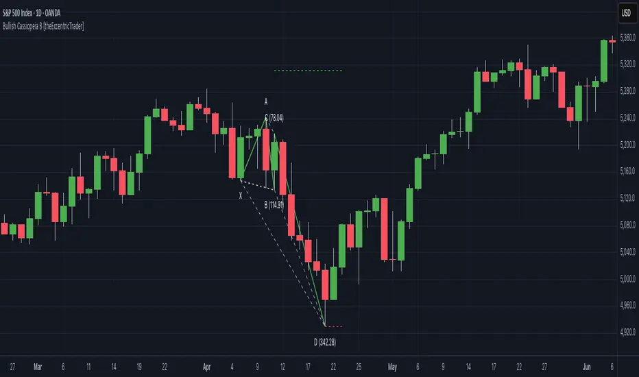
Bearish Cassiopeia A Harmonic Patterns [theEccentricTrader]█ OVERVIEW
This indicator automatically detects and draws bearish Cassiopeia A harmonic patterns and price projections derived from the ranges that constitute the patterns.
Cassiopeia A, B and C harmonic patterns are patterns that I created/discovered myself. They are all inspired by the Cassiopeia constellation and each one is based on different rotations of the constellation as it moves through the sky. The range ratios are also based on the constellation's right ascension and declination listed on Wikipedia:
Right ascension 22h 57m 04.5897s–03h 41m 14.0997s
Declination 77.6923447°–48.6632690°
en.wikipedia.org
I actually developed this idea quite a while ago now but have not felt audacious enough to introduce a new harmonic pattern, let alone 3 at the same time! But I have since been able to run backtests on tick data going back to 2002 across a variety of market and timeframe combinations and have learned that the Cassiopeia patterns can certainly hold their own against the currently known harmonic patterns.
I would also point out that the Cassiopeia constellation does actually look like a harmonic pattern and the Cassiopeia A star is literally the 'strongest source of radio emission in the sky beyond the solar system', so its arguably more of a real harmonic phenomenon than the current patterns.
www.britannica.com
chandra.si.edu
█ CONCEPTS
Green and Red Candles
• A green candle is one that closes with a close price equal to or above the price it opened.
• A red candle is one that closes with a close price that is lower than the price it opened.
Swing Highs and Swing Lows
• A swing high is a green candle or series of consecutive green candles followed by a single red candle to complete the swing and form the peak.
• A swing low is a red candle or series of consecutive red candles followed by a single green candle to complete the swing and form the trough.
Peak and Trough Prices (Basic)
• The peak price of a complete swing high is the high price of either the red candle that completes the swing high or the high price of the preceding green candle, depending on which is higher.
• The trough price of a complete swing low is the low price of either the green candle that completes the swing low or the low price of the preceding red candle, depending on which is lower.
Historic Peaks and Troughs
The current, or most recent, peak and trough occurrences are referred to as occurrence zero. Previous peak and trough occurrences are referred to as historic and ordered numerically from right to left, with the most recent historic peak and trough occurrences being occurrence one.
Range
The range is simply the difference between the current peak and current trough prices, generally expressed in terms of points or pips.
Upper Trends
• A return line uptrend is formed when the current peak price is higher than the preceding peak price.
• A downtrend is formed when the current peak price is lower than the preceding peak price.
• A double-top is formed when the current peak price is equal to the preceding peak price.
Lower Trends
• An uptrend is formed when the current trough price is higher than the preceding trough price.
• A return line downtrend is formed when the current trough price is lower than the preceding trough price.
• A double-bottom is formed when the current trough price is equal to the preceding trough price.
Muti-Part Upper and Lower Trends
• A multi-part return line uptrend begins with the formation of a new return line uptrend and continues until a new downtrend ends the trend.
• A multi-part downtrend begins with the formation of a new downtrend and continues until a new return line uptrend ends the trend.
• A multi-part uptrend begins with the formation of a new uptrend and continues until a new return line downtrend ends the trend.
• A multi-part return line downtrend begins with the formation of a new return line downtrend and continues until a new uptrend ends the trend.
Double Trends
• A double uptrend is formed when the current trough price is higher than the preceding trough price and the current peak price is higher than the preceding peak price.
• A double downtrend is formed when the current peak price is lower than the preceding peak price and the current trough price is lower than the preceding trough price.
Muti-Part Double Trends
• A multi-part double uptrend begins with the formation of a new uptrend that proceeds a new return line uptrend, and continues until a new downtrend or return line downtrend ends the trend.
• A multi-part double downtrend begins with the formation of a new downtrend that proceeds a new return line downtrend, and continues until a new uptrend or return line uptrend ends the trend.
Wave Cycles
A wave cycle is here defined as a complete two-part move between a swing high and a swing low, or a swing low and a swing high. The first swing high or swing low will set the course for the sequence of wave cycles that follow; for example a chart that begins with a swing low will form its first complete wave cycle upon the formation of the first complete swing high and vice versa.
Figure 1.
Retracement and Extension Ratios
Retracement and extension ratios are calculated by dividing the current range by the preceding range and multiplying the answer by 100. Retracement ratios are those that are equal to or below 100% of the preceding range and extension ratios are those that are above 100% of the preceding range.
Fibonacci Retracement and Extension Ratios
The Fibonacci sequence is a series of numbers in which each number is the sum of the two preceding numbers, starting with 0 and 1. For example 0 + 1 = 1, 1 + 1 = 2, 1 + 2 = 3, and so on. Ultimately, we could go on forever but the first few numbers in the sequence are as follows: 0 , 1, 1, 2, 3, 5, 8, 13, 21, 34, 55, 89, 144.
The extension ratios are calculated by dividing each number in the sequence by the number preceding it. For example 0/1 = 0, 1/1 = 1, 2/1 = 2, 3/2 = 1.5, 5/3 = 1.6666..., 8/5 = 1.6, 13/8 = 1.625, 21/13 = 1.6153..., 34/21 = 1.6190..., 55/34 = 1.6176..., 89/55 = 1.6181..., 144/89 = 1.6179..., and so on. The retracement ratios are calculated by inverting this process and dividing each number in the sequence by the number proceeding it. For example 0/1 = 0, 1/1 = 1, 1/2 = 0.5, 2/3 = 0.666..., 3/5 = 0.6, 5/8 = 0.625, 8/13 = 0.6153..., 13/21 = 0.6190..., 21/34 = 0.6176..., 34/55 = 0.6181..., 55/89 = 0.6179..., 89/144 = 0.6180..., and so on.
1.618 is considered to be the 'golden ratio', found in many natural phenomena such as the growth of seashells and the branching of trees. Some now speculate the universe oscillates at a frequency of 0,618 Hz, which could help to explain such phenomena, but this theory has yet to be proven.
Traders and analysts use Fibonacci retracement and extension indicators, consisting of horizontal lines representing different Fibonacci ratios, for identifying potential levels of support and resistance. Fibonacci ranges are typically drawn from left to right, with retracement levels representing ratios inside of the current range and extension levels representing ratios extended outside of the current range. If the current wave cycle ends on a swing low, the Fibonacci range is drawn from peak to trough. If the current wave cycle ends on a swing high the Fibonacci range is drawn from trough to peak.
Harmonic Patterns
The concept of harmonic patterns in trading was first introduced by H.M. Gartley in his book "Profits in the Stock Market", published in 1935. Gartley observed that markets have a tendency to move in repetitive patterns, and he identified several specific patterns that he believed could be used to predict future price movements.
Since then, many other traders and analysts have built upon Gartley's work and developed their own variations of harmonic patterns. One such contributor is Larry Pesavento, who developed his own methods for measuring harmonic patterns using Fibonacci ratios. Pesavento has written several books on the subject of harmonic patterns and Fibonacci ratios in trading. Another notable contributor to harmonic patterns is Scott Carney, who developed his own approach to harmonic trading in the late 1990s and also popularised the use of Fibonacci ratios to measure harmonic patterns. Carney expanded on Gartley's work and also introduced several new harmonic patterns, such as the Shark pattern and the 5-0 pattern.
The bullish and bearish Gartley patterns are the oldest recognized harmonic patterns in trading and all the other harmonic patterns are ultimately modifications of the original Gartley patterns. Gartley patterns are fundamentally composed of 5 points, or 4 waves.
Bullish and Bearish Cassiopeia A Harmonic Patterns
• Bullish Cassiopeia A patterns are fundamentally composed of three troughs and two peaks. The second peak being higher than the first peak. And the third trough being higher than both the first and second troughs, while the second trough is also higher than the first.
• Bearish Cassiopeia A patterns are fundamentally composed of three peaks and two troughs. The second trough being lower than the first trough. And the third peak being lower than both the first and second peaks, while the second peak is also lower than the first.
The ratio measurements I use to detect the patterns are as follows:
• Wave 1 of the pattern, generally referred to as XA, has no specific ratio requirements.
• Wave 2 of the pattern, generally referred to as AB, should retrace by at least 11.34%, but no further than 22.31% of the range set by wave 1.
• Wave 3 of the pattern, generally referred to as BC, should extend by at least 225.7%, but no further than 341% of the range set by wave 2.
• Wave 4 of the pattern, generally referred to as CD, should retrace by at least 77.69%, but no further than 88.66% of the range set by wave 3.
Measurement Tolerances
In general, tolerance in measurements refers to the allowable variation or deviation from a specific value or dimension. It is the range within which a particular measurement is considered to be acceptable or accurate. In this script I have applied this concept to the measurement of harmonic pattern ratios to increase to the frequency of pattern occurrences.
For example, the AB measurement of Gartley patterns is generally set at around 61.8%, but with such specificity in the measuring requirements the patterns are very rare. We can increase the frequency of pattern occurrences by setting a tolerance. A tolerance of 10% to both downside and upside, which is the default setting for all tolerances, means we would have a tolerable measurement range between 51.8-71.8%, thus increasing the frequency of occurrence.
█ FEATURES
Inputs
• AB Lower Tolerance
• AB Upper Tolerance
• BC Lower Tolerance
• BC Upper Tolerance
• CD Lower Tolerance
• CD Upper Tolerance
• Pattern Color
• Label Color
• Show Projections
• Extend Current Projection Lines
Alerts
Users can set alerts for when the patterns occur.
█ LIMITATIONS
All green and red candle calculations are based on differences between open and close prices, as such I have made no attempt to account for green candles that gap lower and close below the close price of the preceding candle, or red candles that gap higher and close above the close price of the preceding candle. This may cause some unexpected behaviour on some markets and timeframes. I can only recommend using 24-hour markets, if and where possible, as there are far fewer gaps and, generally, more data to work with.
█ NOTES
I know a few people have been requesting a single indicator that contains all my patterns and I definitely hear you on that one. However, I have been very busy working on other projects while trying to trade and be a human at the same time. For now I am going to maintain my original approach of releasing each pattern individually so as to maintain consistency. But I am now also working on getting my some of my libraries ready for public release and in doing so I will finally be able to fit all patterns into one script. I will also be giving my scripts some TLC by making them cleaner once I have the libraries up and running. Please bear with me in the meantime, this may take a while. Cheers!
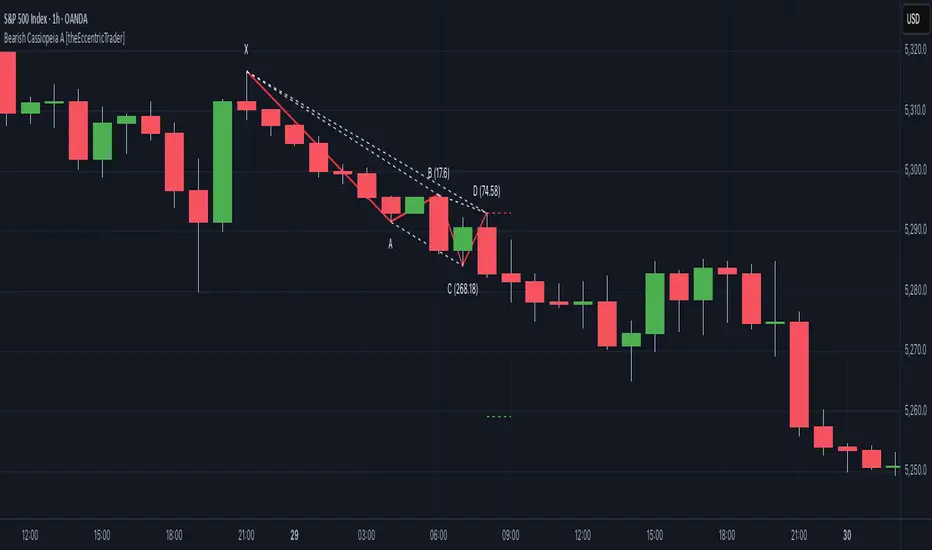
Bullish Cassiopeia A Harmonic Patterns [theEccentricTrader]█ OVERVIEW
This indicator automatically detects and draws bullish Cassiopeia A harmonic patterns and price projections derived from the ranges that constitute the patterns.
Cassiopeia A, B and C harmonic patterns are patterns that I created/discovered myself. They are all inspired by the Cassiopeia constellation and each one is based on different rotations of the constellation as it moves through the sky. The range ratios are also based on the constellation's right ascension and declination listed on Wikipedia:
Right ascension 22h 57m 04.5897s–03h 41m 14.0997s
Declination 77.6923447°–48.6632690°
en.wikipedia.org
I actually developed this idea quite a while ago now but have not felt audacious enough to introduce a new harmonic pattern, let alone 3 at the same time! But I have since been able to run backtests on tick data going back to 2002 across a variety of market and timeframe combinations and have learned that the Cassiopeia patterns can certainly hold their own against the currently known harmonic patterns. As can be seen in the picture above the bullish Cassiopeia A caught the 2009 bear market bottom almost perfectly.
I would also point out that the Cassiopeia constellation does actually look like a harmonic pattern and the Cassiopeia A star is literally the 'strongest source of radio emission in the sky beyond the solar system', so its arguably more of a real harmonic phenomenon than the current patterns.
www.britannica.com
chandra.si.edu
█ CONCEPTS
Green and Red Candles
• A green candle is one that closes with a close price equal to or above the price it opened.
• A red candle is one that closes with a close price that is lower than the price it opened.
Swing Highs and Swing Lows
• A swing high is a green candle or series of consecutive green candles followed by a single red candle to complete the swing and form the peak.
• A swing low is a red candle or series of consecutive red candles followed by a single green candle to complete the swing and form the trough.
Peak and Trough Prices (Basic)
• The peak price of a complete swing high is the high price of either the red candle that completes the swing high or the high price of the preceding green candle, depending on which is higher.
• The trough price of a complete swing low is the low price of either the green candle that completes the swing low or the low price of the preceding red candle, depending on which is lower.
Historic Peaks and Troughs
The current, or most recent, peak and trough occurrences are referred to as occurrence zero. Previous peak and trough occurrences are referred to as historic and ordered numerically from right to left, with the most recent historic peak and trough occurrences being occurrence one.
Range
The range is simply the difference between the current peak and current trough prices, generally expressed in terms of points or pips.
Upper Trends
• A return line uptrend is formed when the current peak price is higher than the preceding peak price.
• A downtrend is formed when the current peak price is lower than the preceding peak price.
• A double-top is formed when the current peak price is equal to the preceding peak price.
Lower Trends
• An uptrend is formed when the current trough price is higher than the preceding trough price.
• A return line downtrend is formed when the current trough price is lower than the preceding trough price.
• A double-bottom is formed when the current trough price is equal to the preceding trough price.
Muti-Part Upper and Lower Trends
• A multi-part return line uptrend begins with the formation of a new return line uptrend and continues until a new downtrend ends the trend.
• A multi-part downtrend begins with the formation of a new downtrend and continues until a new return line uptrend ends the trend.
• A multi-part uptrend begins with the formation of a new uptrend and continues until a new return line downtrend ends the trend.
• A multi-part return line downtrend begins with the formation of a new return line downtrend and continues until a new uptrend ends the trend.
Double Trends
• A double uptrend is formed when the current trough price is higher than the preceding trough price and the current peak price is higher than the preceding peak price.
• A double downtrend is formed when the current peak price is lower than the preceding peak price and the current trough price is lower than the preceding trough price.
Muti-Part Double Trends
• A multi-part double uptrend begins with the formation of a new uptrend that proceeds a new return line uptrend, and continues until a new downtrend or return line downtrend ends the trend.
• A multi-part double downtrend begins with the formation of a new downtrend that proceeds a new return line downtrend, and continues until a new uptrend or return line uptrend ends the trend.
Wave Cycles
A wave cycle is here defined as a complete two-part move between a swing high and a swing low, or a swing low and a swing high. The first swing high or swing low will set the course for the sequence of wave cycles that follow; for example a chart that begins with a swing low will form its first complete wave cycle upon the formation of the first complete swing high and vice versa.
Figure 1.
Retracement and Extension Ratios
Retracement and extension ratios are calculated by dividing the current range by the preceding range and multiplying the answer by 100. Retracement ratios are those that are equal to or below 100% of the preceding range and extension ratios are those that are above 100% of the preceding range.
Fibonacci Retracement and Extension Ratios
The Fibonacci sequence is a series of numbers in which each number is the sum of the two preceding numbers, starting with 0 and 1. For example 0 + 1 = 1, 1 + 1 = 2, 1 + 2 = 3, and so on. Ultimately, we could go on forever but the first few numbers in the sequence are as follows: 0 , 1, 1, 2, 3, 5, 8, 13, 21, 34, 55, 89, 144.
The extension ratios are calculated by dividing each number in the sequence by the number preceding it. For example 0/1 = 0, 1/1 = 1, 2/1 = 2, 3/2 = 1.5, 5/3 = 1.6666..., 8/5 = 1.6, 13/8 = 1.625, 21/13 = 1.6153..., 34/21 = 1.6190..., 55/34 = 1.6176..., 89/55 = 1.6181..., 144/89 = 1.6179..., and so on. The retracement ratios are calculated by inverting this process and dividing each number in the sequence by the number proceeding it. For example 0/1 = 0, 1/1 = 1, 1/2 = 0.5, 2/3 = 0.666..., 3/5 = 0.6, 5/8 = 0.625, 8/13 = 0.6153..., 13/21 = 0.6190..., 21/34 = 0.6176..., 34/55 = 0.6181..., 55/89 = 0.6179..., 89/144 = 0.6180..., and so on.
1.618 is considered to be the 'golden ratio', found in many natural phenomena such as the growth of seashells and the branching of trees. Some now speculate the universe oscillates at a frequency of 0,618 Hz, which could help to explain such phenomena, but this theory has yet to be proven.
Traders and analysts use Fibonacci retracement and extension indicators, consisting of horizontal lines representing different Fibonacci ratios, for identifying potential levels of support and resistance. Fibonacci ranges are typically drawn from left to right, with retracement levels representing ratios inside of the current range and extension levels representing ratios extended outside of the current range. If the current wave cycle ends on a swing low, the Fibonacci range is drawn from peak to trough. If the current wave cycle ends on a swing high the Fibonacci range is drawn from trough to peak.
Harmonic Patterns
The concept of harmonic patterns in trading was first introduced by H.M. Gartley in his book "Profits in the Stock Market", published in 1935. Gartley observed that markets have a tendency to move in repetitive patterns, and he identified several specific patterns that he believed could be used to predict future price movements.
Since then, many other traders and analysts have built upon Gartley's work and developed their own variations of harmonic patterns. One such contributor is Larry Pesavento, who developed his own methods for measuring harmonic patterns using Fibonacci ratios. Pesavento has written several books on the subject of harmonic patterns and Fibonacci ratios in trading. Another notable contributor to harmonic patterns is Scott Carney, who developed his own approach to harmonic trading in the late 1990s and also popularised the use of Fibonacci ratios to measure harmonic patterns. Carney expanded on Gartley's work and also introduced several new harmonic patterns, such as the Shark pattern and the 5-0 pattern.
The bullish and bearish Gartley patterns are the oldest recognized harmonic patterns in trading and all the other harmonic patterns are ultimately modifications of the original Gartley patterns. Gartley patterns are fundamentally composed of 5 points, or 4 waves.
Bullish and Bearish Cassiopeia A Harmonic Patterns
• Bullish Cassiopeia A patterns are fundamentally composed of three troughs and two peaks. The second peak being higher than the first peak. And the third trough being higher than both the first and second troughs, while the second trough is also higher than the first.
• Bearish Cassiopeia A patterns are fundamentally composed of three peaks and two troughs. The second trough being lower than the first trough. And the third peak being lower than both the first and second peaks, while the second peak is also lower than the first.
The ratio measurements I use to detect the patterns are as follows:
• Wave 1 of the pattern, generally referred to as XA, has no specific ratio requirements.
• Wave 2 of the pattern, generally referred to as AB, should retrace by at least 11.34%, but no further than 22.31% of the range set by wave 1.
• Wave 3 of the pattern, generally referred to as BC, should extend by at least 225.7%, but no further than 341% of the range set by wave 2.
• Wave 4 of the pattern, generally referred to as CD, should retrace by at least 77.69%, but no further than 88.66% of the range set by wave 3.
Measurement Tolerances
In general, tolerance in measurements refers to the allowable variation or deviation from a specific value or dimension. It is the range within which a particular measurement is considered to be acceptable or accurate. In this script I have applied this concept to the measurement of harmonic pattern ratios to increase to the frequency of pattern occurrences.
For example, the AB measurement of Gartley patterns is generally set at around 61.8%, but with such specificity in the measuring requirements the patterns are very rare. We can increase the frequency of pattern occurrences by setting a tolerance. A tolerance of 10% to both downside and upside, which is the default setting for all tolerances, means we would have a tolerable measurement range between 51.8-71.8%, thus increasing the frequency of occurrence.
█ FEATURES
Inputs
• AB Lower Tolerance
• AB Upper Tolerance
• BC Lower Tolerance
• BC Upper Tolerance
• CD Lower Tolerance
• CD Upper Tolerance
• Pattern Color
• Label Color
• Show Projections
• Extend Current Projection Lines
Alerts
Users can set alerts for when the patterns occur.
█ LIMITATIONS
All green and red candle calculations are based on differences between open and close prices, as such I have made no attempt to account for green candles that gap lower and close below the close price of the preceding candle, or red candles that gap higher and close above the close price of the preceding candle. This may cause some unexpected behaviour on some markets and timeframes. I can only recommend using 24-hour markets, if and where possible, as there are far fewer gaps and, generally, more data to work with.
█ NOTES
I know a few people have been requesting a single indicator that contains all my patterns and I definitely hear you on that one. However, I have been very busy working on other projects while trying to trade and be a human at the same time. For now I am going to maintain my original approach of releasing each pattern individually so as to maintain consistency. But I am now also working on getting my some of my libraries ready for public release and in doing so I will finally be able to fit all patterns into one script. I will also be giving my scripts some TLC by making them cleaner once I have the libraries up and running. Please bear with me in the meantime, this may take a while. Cheers!