CCI Multi-TimeframeThe Commodity Channel Index (CCI) is a leading oscillating momentum indicator that was developed by Donald Lambert to identify cyclical turns in commodities but can also be used on securities and bonds as well.
HOW IS IT USED ?
Lambert used the CCI to generate entry and exit signals when the CCI moved above +100% and below -100% respectively. When the CCI moves above +100%, the security enters into a strong uptrend and an entry signal is given. When the CCI moves back below +100% this position should be closed. Conversely, when the CCI moves below -100%, the security enters into a strong downtrend and an exit signal is given. When the CCI moves back above -100% this position should be closed.
In addition, an entry signal is given when the CCI bounces off of the zero line. When the CCI reaches the zero line, the security's average price is at the moving average used to calculate the CCI and when a security bounces off its moving average it is considered a good entry position as the security has pulled back to its short-term support with the bounce reaffirming the current trend.
The CCI can also be used to identify overbought and oversold levels. A security could be considered oversold when the CCI moves below -100 and overbought when it moves above +100. From an oversold level, an entry signal may be given when the CCI moves above -100. From an overbought level, an exit signal might be given when the CCI moves below +100.
Divergences can also be applied to the CCI. A positive divergence below -100 would increase the probability of a signal based on a move above -100, and a negative divergence above +100 would increase the probability of a signal based on a move back below +100.
Trend line breaks can be used to generate entry and exit signals. Trend lines can be drawn connecting the peaks and troughs. From oversold levels, a move above -100 and a trend line breakout could be used as an entry signal. Conversely, from overbought levels, a move below +100 and a trend line breakout could be used as an exit signal.
I added the possibility to add on the chart a 2nd timeframe for confirmation.
If you found this script useful, a tip is always welcome... :)
在脚本中搜索"100年国际黄金价格"

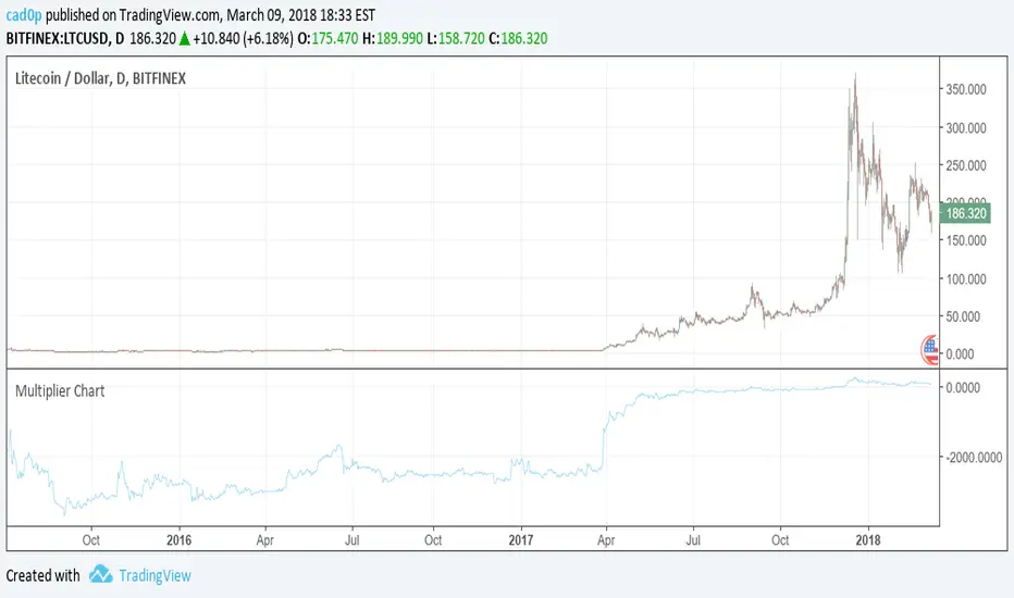
Multiplier ChartI am proposing an alternative to the percent change.
An alternative that is symmetrical to both positive and negative change, unlike percentage change.
The simple idea is to have a positive number if the reference value (called val in the script) is lower than the stock value and needs to be multiplied;
a negative number instead if the reference number is higher than the stock value, so the reference value needs to be divided.
Multiplying all by 100 to give clearer and more readable results, the Multiplier would have a huge gap between +100 and -100, because a stock multiplied by 1 or divided by 1 are the same thing.
So we need to compromise and move all positive numbers down by 100 and all negative numbers up by 100. This actually gives a similar result to percentage change, and it is actually identical in the positive range.
The fundamental difference lies on the negative range, which is completely symmetrical. So if a stock goes up 100 points one day (doubles), and the next it goes down another 100 points (halves), at the end of the second day the stock has the same value as it had at the beginning of the first day! On percentage change it would be +100% the first day and -50% the second.
We mustn't undervalue the human tendency to compare a 1% change to a -1% change, but they do not mean the same even if they seem to indicate so.
A clear example of this can be found on CMC 0.60% -3.56% -3.56% (CoinMarketCap), in which each day are shown the best and worst performing coins of the day. So you might see a +900% there in the top performing, but you'll never see a -900%, because percentage change cannot go further than -100%. It is a fundamentally asymmetric scale that can confuse people a lot especially in those fast moving new markets.ù
I am welcome to feedback and all kinds of opinions and critics.
Some interesting things to note: you can use it as a percentage change indicator or as a different perspective to a stock chart. In fact, it lets you see how big of a difference it made buying coins when they were very cheap, because when they are cheap a difference of what it might seem nothing is amplified by all the gains that the stock/coin made after. So, looking at coins charts using this indicator shows how "not flat" were the early days, which in a normal chart are flattened to 0.
SNIPER ORB V2# 🎯 SNIPER ORB TRADING CHEAT SHEET
## Quick Reference Guide for Live Trading
---
## 📊 VISUAL IDENTIFICATION GUIDE
```
═══════════════════════════════════════════════════════════════════
YOUR CHART AT A GLANCE
═══════════════════════════════════════════════════════════════════
🔵 BRIGHT BLUE LINES (3px) → 5min ORB High/Low
🔷 CYAN LINES (2px) → 15min ORB High/Low
🟣 PURPLE LINES (2px) → 30min ORB High/Low (PRIMARY)
🟢 GREEN DASHED LINES (1px) → Upside targets (1x, 2x, 3x from 30min ORB)
🔴 RED DASHED LINES (1px) → Downside targets (1x, 2x, 3x from 30min ORB)
🟡 GOLD LINE (2px) → Anchored VWAP (9:30 AM anchor for NY, 3:00 AM for London)
📋 INFO TABLE (top-right) → Shows live ORB ranges, VWAP price, status
═══════════════════════════════════════════════════════════════════
```
**KEY DIFFERENCE FROM OTHER ORB INDICATORS:**
- You see **ALL 3 ORB PERIODS SIMULTANEOUSLY** (5min, 15min, 30min)
- Targets calculated from **30min ORB ONLY** (not 5min or 15min)
- **NO BOX FILLS** - clean line-only display for sniper precision
- Auto-disappears at session end (no clutter from old sessions)
---
## 🔘 NEW FEATURE: ORB DISPLAY TOGGLES
**You now have FULL CONTROL over which ORB periods to display!**
```
In indicator settings → "ORB Display" section:
☑ Show 5min ORB → Toggle blue lines ON/OFF
☑ Show 15min ORB → Toggle cyan lines ON/OFF
☑ Show 30min ORB → Toggle purple lines ON/OFF
USE CASES:
━━━━━━━━━━━━━━━━━━━━━━━━━━━━━━━━━━━━━━━━━━━━━━━
1. FOCUS MODE (30min only)
☐ 5min ☐ 15min ☑ 30min
→ Clean chart, just your primary trading range
→ Best for beginners or minimalist traders
2. EARLY WARNING MODE (5min + 30min)
☑ 5min ☐ 15min ☑ 30min
→ See early breaks with 5min, trade 30min confirmation
→ Reduces visual noise from 15min
3. CONFLUENCE MODE (all 3 ORBs)
☑ 5min ☑ 15min ☑ 30min
→ Maximum information, all alignment signals
→ For advanced traders seeking highest probability
4. INTRADAY SCALP MODE (5min only)
☑ 5min ☐ 15min ☐ 30min
→ Ultra-fast entries on 5min breaks
→ High-risk, high-frequency approach
━━━━━━━━━━━━━━━━━━━━━━━━━━━━━━━━━━━━━━━━━━━━━━━
💡 PRO TIP: Start with 30min only, then add 5min/15min as you gain experience
```
---
## 🎯 FIXED: ANCHORED VWAP (TIMESTAMP-BASED)
**The VWAP now anchors with SURGICAL PRECISION to the exact session start candle!**
```
LONDON SESSION:
• Anchors at the EXACT 3:00 AM ET candle
• Uses timestamp checking: hour == 3 AND minute == 0
• Resets every morning at London Open
NEW YORK SESSION:
• Anchors at the EXACT 9:30 AM ET candle
• Uses timestamp checking: hour == 9 AND minute == 30
• Resets every day at NY Open
WHAT THIS MEANS:
✅ VWAP starts accumulating from the first tick of the session
✅ No more "off by one bar" errors
✅ Institutional-grade VWAP anchoring
✅ Perfect alignment with your ORB start times
HOW TO VERIFY IT'S WORKING:
1. Load indicator on 1min or 5min chart
2. Find the exact 9:30 AM candle (NY) or 3:00 AM candle (London)
3. VWAP should START appearing from that exact bar
4. Not the bar before, not the bar after - THAT EXACT BAR
```
---
## ⏰ SESSION TIMING MATRIX
| Session | Start Time | 5min Complete | 15min Complete | 30min Complete | Session End |
|---------|-----------|---------------|----------------|----------------|-------------|
| **London** | 3:00 AM ET | 3:05 AM | 3:15 AM | 3:30 AM | 9:30 AM ET (disappears) |
| **New York** | 9:30 AM ET | 9:35 AM | 9:45 AM | 10:00 AM | 5:00 PM ET (disappears) |
**💡 GOLDEN RULES:**
1. **WAIT FOR 30MIN ORB TO COMPLETE** before trading targets (10:00 AM NY / 3:30 AM London)
2. Use 5min and 15min ORBs as **early warning signals** only
3. All ORB lines + VWAP **auto-delete** at session end (clean chart)
---
## 🎯 THE 3-ORB SYSTEM: HOW IT WORKS
### **Hierarchical ORB Structure**
```
TIME: 9:30 AM ─────────────────────────────────> 10:00 AM ──────> 5:00 PM
↓ ↓
SESSION START 30min ORB COMPLETE
(all 3 ORBs begin forming) (targets appear)
📍 5min ORB (9:30-9:35 AM): ━━━━━━━━━━━━━━━━━━━━━━━━━━━━━━━━━━━━━>
Purpose: EARLY breakout signal, fastest-moving boundary
📍 15min ORB (9:30-9:45 AM): ━━━━━━━━━━━━━━━━━━━━━━━━━━━━━━━━━━━━━>
Purpose: MID-TERM institutional reference level
📍 30min ORB (9:30-10:00 AM): ━━━━━━━━━━━━━━━━━━━━━━━━━━━━━━━━━━━━━>
Purpose: PRIMARY TRADING RANGE - all targets calculated from this
🎯 TARGETS (10:00 AM onward): ▪ ▪ ▪ ▪ ▪ (1x, 2x, 3x from 30min ORB)
Purpose: Profit-taking levels based on 30min range
```
**Why 3 ORBs Instead of 1?**
- **5min ORB**: Captures early institutional positioning (first 5 minutes)
- **15min ORB**: Confirms directional bias (more stable than 5min)
- **30min ORB**: Full market digestion of overnight news + opening orders
- **Confluence = Higher Win Rate**: When all 3 align, breakouts are extremely reliable
---
## 🎯 THE 5 HIGH-PROBABILITY SETUPS
### **SETUP #1: TRIPLE ORB BREAKOUT CONFLUENCE** ⭐⭐⭐⭐⭐
```
CONDITIONS:
✅ 30min ORB complete (10:00 AM NY / 3:30 AM London)
✅ Price breaks ALL 3 ORBs simultaneously:
• 5min high/low (blue line)
• 15min high/low (cyan line)
• 30min high/low (purple line)
✅ VWAP confirms direction (below price = bullish, above = bearish)
✅ Volume spike on breakout candle
ENTRY: Close of breakout candle (must close beyond ALL 3 ORBs)
STOP: Inside 30min ORB at 30m low (long) or 30m high (short)
TARGET 1: First green/red dashed line (0.5x 30m range)
TARGET 2: Second target (1x 30m range)
TARGET 3: Third target (1.5x 30m range)
WIN RATE: 75-85% | R:R = 1:2.5 minimum
NOTES: When all 3 ORBs align, institutional order flow is unanimous
```
---
### **SETUP #2: 5MIN EARLY BREAKOUT → 30MIN CONFIRMATION** ⭐⭐⭐⭐
```
CONDITIONS:
✅ Price breaks 5min ORB first (blue line crossed)
✅ 15min ORB holds initially (cyan line not crossed yet)
✅ After 30min ORB completes, price breaks 30min boundary (purple)
✅ VWAP alignment confirms direction
✅ All 3 ORBs now broken in same direction
ENTRY: When 30min ORB breaks (purple line) + 5min/15min already broken
STOP: 30min ORB opposite boundary
TARGET 1-3: Standard targets from 30min ORB
WIN RATE: 70-80% | R:R = 1:2+
NOTES: 5min gave early warning, 30min confirms institutional commitment
```
---
### **SETUP #3: FALSE 5MIN BREAKOUT → 30MIN REVERSAL** ⭐⭐⭐⭐⭐
```
CONDITIONS:
✅ Price breaks 5min ORB (blue line)
✅ Fails to break 15min or 30min ORBs (cyan/purple lines hold)
✅ Price reverses back inside 5min ORB
✅ Then breaks OPPOSITE side of 30min ORB (purple line)
✅ VWAP flips to confirm new direction
ENTRY: When 30min ORB breaks in OPPOSITE direction of failed 5min break
STOP: Failed 5min breakout high/low (now a liquidity grab zone)
TARGET 1-3: Standard targets
WIN RATE: 80-90% | R:R = 1:3+ (trapped traders forced to exit)
NOTES: Most profitable setup - 5min breakout was liquidity hunt
```
---
### **SETUP #4: TIGHT COMPRESSION → EXPLOSION** ⭐⭐⭐⭐
```
CONDITIONS:
✅ All 3 ORBs tightly overlapping (5m, 15m, 30m within 50 points on YM)
✅ Range < 0.3% of price (very tight consolidation)
✅ VWAP sitting in middle of compression
✅ 30min ORB complete, price still inside all 3
ENTRY: Simultaneous break of ALL 3 ORBs + VWAP cross
STOP: Middle of compression zone
TARGET: 2x-4x normal targets (volatility expansion)
WIN RATE: 65-75% | R:R = 1:5+ (explosive breakout)
NOTES: Low volatility → high volatility shift, institutions coiling spring
```
---
### **SETUP #5: VWAP BOUNCE WITHIN 30MIN ORB** ⭐⭐⭐⭐
```
CONDITIONS:
✅ Price stayed inside 30min ORB for 1+ hours post-formation
✅ VWAP acting as dynamic support (long) or resistance (short)
✅ Price bouncing between VWAP and 30min ORB boundaries
✅ Clear rejection candles at VWAP
ENTRY: When price bounces off VWAP toward 30min ORB boundary
• Long: VWAP bounce up toward 30m high (purple)
• Short: VWAP rejection down toward 30m low (purple)
STOP: Beyond VWAP by 20 points
TARGET: 30min ORB opposite boundary
WIN RATE: 70-80% | R:R = 1:1.5-2
NOTES: Range-bound play, NOT for breakout traders
```
---
## 🛡️ RISK MANAGEMENT RULES
### **Position Sizing by ORB Range**
```
30min ORB Range | Stop Distance | Risk $500 (1%) | YM Contracts
-----------------|------------------|-----------------|-------------
< 50 points | 50 pts | $500 ÷ $250 = | 2 contracts
50-100 points | 100 pts | $500 ÷ $500 = | 1 contract
100-150 points | 150 pts | $500 ÷ $750 = | 0.66 (use 1)
150-200 points | 200 pts | $500 ÷ $1000 = | 0.5 (use 1)
> 200 points | Don't trade | Too wide | Skip setup
Formula: Risk $ ÷ (Stop Distance × $5 per YM point) = Max Contracts
```
### **The 3-Strike Rule (MANDATORY)**
```
✅ Trade 1: Full position size (based on 30m ORB range)
❌ Stop hit → Trade 2: HALF position size
❌ Stop hit → Trade 3: QUARTER position size
❌ Stop hit → DONE FOR THE DAY (no exceptions)
```
### **Profit Taking Ladder**
```
TARGET 1 (0.5x 30m range): Take 50% off, move stop to breakeven
TARGET 2 (1.0x 30m range): Take 30% off, trail stop by 25 points
TARGET 3 (1.5x 30m range): Take 15% off, let 5% run with 50pt trail
```
---
## ⚠️ DO NOT TRADE IF...
```
🚫 30min ORB incomplete (< 10:00 AM NY / < 3:30 AM London)
🚫 30min ORB range < 40 points YM (too tight, likely chop)
🚫 30min ORB range > 250 points YM (too wide, unpredictable)
🚫 All 3 ORBs wildly divergent (5m=100pts, 15m=180pts, 30m=240pts)
🚫 Major news release within 30 minutes (wait for ORB to reform)
🚫 You've hit 3 losses in the session (3-strike rule)
🚫 You're tired, emotional, revenge trading, or distracted
🚫 Time > 12:00 PM ET (lunch, avoid until 1:00 PM)
🚫 Time > 3:00 PM ET unless Power Hour (3:00-4:00 PM) momentum
```
---
## 🔍 PRE-SESSION CHECKLIST
**15 Minutes Before London (2:45 AM ET) or NY (9:15 AM ET):**
```
□ Check economic calendar (FOMC? NFP? CPI? → extra caution)
□ Review previous session's ORB ranges (context for today's volatility)
□ Load SNIPER ORB on 1min or 5min chart
□ Select correct session: "London" or "New York"
□ Verify indicator settings:
• Number of Targets: 3
• Target % of 30min Range: 50%
• Show Anchored VWAP: ON
□ Set TradingView alerts:
• 30min ORB complete (10:00 AM or 3:30 AM)
• Price crossing 30min high/low
• VWAP crosses
□ Prepare bracket orders mentally (entry, stop, 3 targets)
□ Review yesterday's P&L and lessons learned
□ Set phone to "Do Not Disturb" mode
```
---
## 🎨 INDICATOR SETTINGS GUIDE
### **Core Settings (Updated with Toggles)**
```
SESSION SETTINGS:
━━━━━━━━━━━━━━━━━━━━━━━━━━━━━━━━━━━━━━━━
• Active Session: "London" or "New York"
ORB DISPLAY (NEW!):
━━━━━━━━━━━━━━━━━━━━━━━━━━━━━━━━━━━━━━━━
☑ Show 5min ORB (toggle blue lines)
☑ Show 15min ORB (toggle cyan lines)
☑ Show 30min ORB (toggle purple lines)
💡 Turn OFF any ORB to declutter your chart!
TARGET SETTINGS:
━━━━━━━━━━━━━━━━━━━━━━━━━━━━━━━━━━━━━━━━
• Number of Targets: 3 (default)
• Target % of 30min Range: 50% (default)
VWAP SETTINGS:
━━━━━━━━━━━━━━━━━━━━━━━━━━━━━━━━━━━━━━━━
☑ Show Anchored VWAP
• VWAP Color: Gold (#FFC107)
• VWAP Width: 2px
```
### **Color Customization (Optimized for Dark Charts)**
```
DEFAULT COLORS:
━━━━━━━━━━━━━━━━━━━━━━━━━━━━━━━━━━━━━━━━
5min ORB: Bright Blue (#2196F3) - 3px wide
15min ORB: Cyan (#00BCD4) - 2px wide
30min ORB: Purple (#9C27B0) - 2px wide
Upside Targets: Green (#4CAF50) - 1px dashed
Downside Targets: Red (#F44336) - 1px dashed
VWAP: Gold (#FFC107) - 2px solid
━━━━━━━━━━━━━━━━━━━━━━━━━━━━━━━━━━━━━━━━
WHY THESE COLORS?
• Blue family (5m/15m) = short-term, high-frequency
• Purple (30m) = primary, institutional level
• Green/Red = universal up/down
• Gold VWAP = fair value anchor (stands out)
```
### **Settings by Trading Style**
**BEGINNER (Clean & Simple):**
```
ORB Display:
☐ Show 5min ORB
☐ Show 15min ORB
☑ Show 30min ORB (30min only - focus mode)
Number of Targets: 2-3
Target % of 30min Range: 50%
Chart Timeframe: 5-minute
```
**SCALPER (5-15 min holds):**
```
ORB Display:
☑ Show 5min ORB (early signals)
☐ Show 15min ORB
☑ Show 30min ORB (confirmation)
Number of Targets: 5
Target % of 30min Range: 30-40%
Label Size: Tiny
Chart Timeframe: 1-minute
```
**DAY TRADER (30-90 min holds):**
```
ORB Display:
☑ Show 5min ORB
☑ Show 15min ORB
☑ Show 30min ORB (all 3 - confluence mode)
Number of Targets: 3
Target % of 30min Range: 50%
Label Size: Small
Chart Timeframe: 5-minute (RECOMMENDED)
```
**SWING TRADER (2-4 hour holds):**
```
ORB Display:
☐ Show 5min ORB (too noisy for swings)
☑ Show 15min ORB
☑ Show 30min ORB
Number of Targets: 2-3
Target % of 30min Range: 75-100%
Label Size: Normal
Chart Timeframe: 15-minute
```
---
## 📈 TIMEFRAME SELECTION GUIDE
| Your Timeframe | What You See | Best For |
|---------------|--------------|----------|
| **1-minute** | Every tick, high noise | Scalping, precision entries |
| **5-minute** | Balanced clarity | Day trading (RECOMMENDED) |
| **15-minute** | Clean structure | Swing positions |
| **30-minute** | Too compressed | Not recommended (can't see ORB form) |
**💡 PRO TIP:**
- **Primary chart: 5-minute** (for entries and monitoring)
- **Secondary chart: 1-minute** (for precise timing)
- **Never go above 15-minute** (ORBs won't form properly)
---
## 🧠 READING THE 3-ORB STRUCTURE
### **Bullish Alignment Patterns**
```
PATTERN 1: "Staircase Expansion"
5min: ━━━━ (tight, 60 pts)
15min: ━━━━━━ (wider, 90 pts)
30min: ━━━━━━━━ (widest, 120 pts)
→ Bullish expansion, expect upside breakout
PATTERN 2: "Nested Compression"
5min: ━━ (30 pts)
15min: ━━━ (35 pts)
30min: ━━━━ (40 pts)
→ All tight, explosive breakout likely
PATTERN 3: "Early Commitment"
5min: ━━━━━━ (100 pts, already broken up)
15min: ━━━━━ (80 pts, holding)
30min: ━━━━━ (110 pts, about to break)
→ 5min led the way, 30min confirmation coming
```
### **Bearish Alignment Patterns**
```
PATTERN 1: "Waterfall Setup"
5min: ━━━━ (50 pts, broke down)
15min: ━━━━━ (70 pts, broke down)
30min: ━━━━━━ (90 pts, about to break)
→ Sequential breakdown, strong bearish momentum
PATTERN 2: "Failed Highs"
5min: ━━━━━━ (upper wick rejections)
15min: ━━━━━━ (couldn't break)
30min: ━━━━━━━ (topped out)
→ All 3 rejecting highs, bearish reversal likely
```
### **Neutral/Chop Patterns (AVOID TRADING)**
```
PATTERN 1: "Wide Divergence"
5min: ━━ (30 pts)
15min: ━━━━━━━ (120 pts)
30min: ━━━━━━━━━━━ (200 pts)
→ No consensus, unpredictable, skip
PATTERN 2: "Whipsaw City"
• Price breaking 5min up, then down, then up again
• 15min and 30min not aligned
• VWAP getting crossed every 5 minutes
→ Chop day, step aside, wait for clarity
```
---
## 📊 INTEGRATION WITH YM ULTIMATE SNIPER v8.1
**The 2-System Confluence Method:**
```
┌─────────────────────────────────────────────────────────────┐
│ STEP 1: SNIPER ORB → Defines "Zones That Matter" │
│ • 30min ORB = primary institutional range │
│ • VWAP = fair value anchor │
│ • Targets = profit zones │
│ • 5min/15min = early warning signals │
└─────────────────────────────────────────────────────────────┘
↓
┌─────────────────────────────────────────────────────────────┐
│ STEP 2: YM ULTIMATE SNIPER → Triggers precise entry │
│ • Wait for GOD MODE signal AT 30min ORB boundary │
│ • 6-gate filter: Score ≥9, fat body ≥70%, delta ≥70% │
│ • Candle Dominance Index (CDI) ≥7 │
│ • Intrabar pressure consistent throughout formation │
└─────────────────────────────────────────────────────────────┘
↓
┌─────────────────────────────────────────────────────────────┐
│ STEP 3: EXECUTE TRADE │
│ • ORB breakout + GOD MODE = MAXIMUM PROBABILITY │
│ • Enter ONLY when BOTH systems align │
│ • This is TRUE "sniper" trading (2-5 trades/day max) │
└─────────────────────────────────────────────────────────────┘
```
**Confluence Scoring for Combined System:**
```
SNIPER ORB Criteria:
□ 30min ORB complete (10:00 AM+) +2 points
□ All 3 ORBs broken in same direction +2 points
□ VWAP alignment (below=bull, above=bear) +1 point
□ Volume spike on breakout candle +1 point
□ Tight 3-ORB compression (<100pt divergence) +1 point
YM ULTIMATE SNIPER Criteria:
□ GOD MODE signal at ORB boundary +3 points
□ Score ≥9.0 (tier classification) +1 point
□ Candle Dominance Index (CDI) ≥8 +1 point
TOTAL POSSIBLE: 12 points
TRADE EXECUTION RULES:
• 10-12 points = MAX SIZE (this is the holy grail setup)
• 8-9 points = FULL SIZE (high probability)
• 6-7 points = HALF SIZE (moderate probability)
• <6 points = NO TRADE (wait for better alignment)
```
---
## 💡 COMMON MISTAKES & FIXES
```
❌ MISTAKE: Trading before 30min ORB completes
✅ FIX: Wait until 10:00 AM (NY) or 3:30 AM (London), NO EXCEPTIONS
❌ MISTAKE: Ignoring 5min and 15min ORBs (only watching 30min)
✅ FIX: Use all 3 for confluence - they're your early warning system
❌ MISTAKE: Chasing breakouts 100+ points beyond 30min ORB
✅ FIX: Wait for pullback to VWAP or 30min boundary for re-entry
❌ MISTAKE: Not adjusting target % for market conditions
✅ FIX: Volatile day (ORB >200pts)? Use 75-100% targets
Calm day (ORB <80pts)? Use 30-40% targets
❌ MISTAKE: Trading when all 3 ORBs are wildly different sizes
✅ FIX: Skip the day if 5m/15m/30m diverge by >100pts - no consensus
❌ MISTAKE: Forgetting VWAP position
✅ FIX: VWAP MUST confirm bias:
• Long: price > VWAP
• Short: price < VWAP
• If VWAP contradicts, skip the trade
❌ MISTAKE: Not respecting the 3-strike rule
✅ FIX: 3 losses = DONE for the session, no rationalization
❌ MISTAKE: Trading during lunch (12:00-1:00 PM ET)
✅ FIX: Volume dies, ORBs lose relevance, false signals increase
```
---
## 🔔 ALERT SETUP (ESSENTIAL)
**TradingView Alerts You MUST Set:**
```
ALERT 1: "30min ORB Complete"
• Type: Time-based
• Trigger: 10:00 AM ET (NY) or 3:30 AM ET (London)
• Message: "🎯 30min ORB complete - targets now active"
ALERT 2: "30min ORB High Breakout"
• Type: Crossing Up
• Value 1: Close
• Value 2: 30min ORB High (purple line)
• Message: "🚀 30m ORB HIGH broken - check for long setup"
ALERT 3: "30min ORB Low Breakdown"
• Type: Crossing Down
• Value 1: Close
• Value 2: 30min ORB Low (purple line)
• Message: "📉 30m ORB LOW broken - check for short setup"
ALERT 4: "VWAP Cross"
• Type: Crossing
• Value 1: Close
• Value 2: VWAP
• Message: "⚡ VWAP crossed - check institutional bias shift"
ALERT 5: "Target 1 Hit"
• Type: Crossing
• Value 1: High (for longs) or Low (for shorts)
• Value 2: First target line
• Message: "🎯 Target 1 hit - take 50% off, move stop to BE"
```
---
## 📱 MOBILE TRADING WORKFLOW
**TradingView Mobile App Setup:**
```
1. SAVE LAYOUT
• Chart: 5-minute timeframe
• SNIPER ORB indicator loaded
• YM Ultimate SNIPER v8.1 loaded (if using)
• Save as "SNIPER ORB - YM"
2. ENABLE NOTIFICATIONS
• Settings → Notifications → Push Alerts: ON
• All 5 alerts above configured
3. QUICK ACCESS
• Add YM futures to Watchlist: "MYM" or "YM1!"
• Pin SNIPER ORB layout to favorites
4. EXECUTION READY
• Broker app (TastyTrade, NinjaTrader, etc.) logged in
• Preset bracket orders:
- Entry: market order
- Stop: 30m ORB opposite boundary
- Targets: 3 levels (50%, 30%, 20% of position)
5. BATTERY & CONNECTIVITY
• Phone charged 100% before session
• Stable WiFi or LTE connection
• Backup power bank available
```
---
## 🎓 DAILY PERFORMANCE JOURNAL
**After Each Trading Session (MANDATORY):**
```
═══════════════════════════════════════════════════════════════
DATE: __________ SESSION: □ London □ New York
═══════════════════════════════════════════════════════════════
ORB DATA:
• 5min ORB Range: ______ points
• 15min ORB Range: ______ points
• 30min ORB Range: ______ points
• Alignment: □ Tight □ Moderate □ Wide (skip if wide)
VWAP BEHAVIOR:
• Opening position: □ Above price □ Below price □ Mixed
• Did VWAP act as support/resistance? □ Yes □ No
TRADES TAKEN:
Total Setups Identified: _____
Trades Executed: _____
Win/Loss Record: _____ W / _____ L
Win Rate: _____%
Gross P&L: $_______
Net P&L (after commissions): $_______
BEST TRADE:
• Setup: ____________________ (which of the 5 setups?)
• Entry Price: ______ Exit Price: ______
• Profit: $_______
• What went RIGHT: _________________________________
_________________________________________________
WORST TRADE:
• Setup: ____________________
• Entry Price: ______ Exit Price: ______
• Loss: $_______
• What went WRONG: _________________________________
_________________________________________________
• Lesson Learned: ___________________________________
3-STRIKE RULE STATUS:
□ No losses (great day)
□ 1 loss (still in game)
□ 2 losses (caution, half size)
□ 3 losses (stopped for day, as required)
TOMORROW'S ADJUSTMENTS:
□ _________________________________________________
□ _________________________________________________
□ _________________________________________________
EMOTIONAL STATE TODAY:
□ Calm & focused (optimal)
□ Anxious/rushed (need to work on patience)
□ Overconfident (dial back position size)
□ Fearful (review winning trades to build confidence)
═══════════════════════════════════════════════════════════════
```
---
## 🚀 YOUR FIRST LIVE TRADE WALKTHROUGH
**Step-by-Step for New York Session (Most Common):**
```
⏰ 9:15 AM ET - PREPARATION
□ Load SNIPER ORB on YM 5-minute chart
□ Select "New York" session in indicator settings
□ Verify VWAP is showing (gold line)
□ Check economic calendar (any big news at 9:30?)
□ Prepare mentally: "I will wait for 30min ORB to complete"
⏰ 9:30 AM ET - SESSION OPENS
□ Watch 3 ORBs begin forming:
• Blue lines (5min) will lock in at 9:35 AM
• Cyan lines (15min) will lock in at 9:45 AM
• Purple lines (30min) will lock in at 10:00 AM
□ Observe VWAP anchoring at 9:30 AM candle
□ DO NOT TRADE YET - just observe
⏰ 9:35 AM - 5MIN ORB COMPLETE
□ Note 5min high/low (blue lines locked)
□ Check info table: "5m Range = XX points"
□ If 5min ORB breaks early, note direction but DON'T ENTER
⏰ 9:45 AM - 15MIN ORB COMPLETE
□ Note 15min high/low (cyan lines locked)
□ Compare to 5min ORB: Aligned? Expanding?
□ Still waiting... patience pays
⏰ 10:00 AM - 30MIN ORB COMPLETE (TARGETS APPEAR!)
□ Purple lines locked (30m high/low)
□ Green/red dashed target lines appear automatically
□ Info table shows "Status: ✓ Complete"
□ NOW you can trade breakouts
⏰ 10:00 AM - 11:30 AM - TRADING WINDOW
□ Wait for price to break purple line (30m ORB high or low)
□ Confirm:
1. All 3 ORBs broken in same direction?
2. VWAP confirming (below=bullish, above=bearish)?
3. Volume spike visible?
4. YM SNIPER GOD MODE signal? (if using)
□ If all YES → ENTER TRADE:
• Market order at breakout close
• Stop at 30m ORB opposite boundary
• Targets at green/red dashed lines
⏰ TARGET MANAGEMENT
□ Price hits first target (1x) → Take 50% off, move stop to BE
□ Price hits second target (2x) → Take 30% off, trail stop
□ Price hits third target (3x) → Take 15% off, let 5% run
⏰ 12:00 PM - LUNCH (AVOID TRADING)
□ Volume dies down
□ ORBs become less relevant
□ Take a break, review morning trades
⏰ 1:00 PM - 3:00 PM - AFTERNOON SESSION
□ ORBs still valid but less reliable
□ Consider waiting for Power Hour (3:00-4:00 PM)
⏰ 5:00 PM - SESSION END
□ All ORB lines disappear automatically
□ VWAP disappears automatically
□ Chart cleans itself - ready for tomorrow
□ Fill out daily journal
```
---
## 🏆 WINNING MINDSET AFFIRMATIONS
Read these BEFORE each trading session:
```
"I trade ORBs, not chaos. Structure gives me edge."
"3 high-quality trades beat 20 mediocre ones."
"The 30min ORB is my anchor. I wait for it. Every. Single. Time."
"When all 3 ORBs align, institutions are unified. I follow."
"VWAP is my institutional compass. I respect its guidance."
"3 strikes and I'm out. Discipline > Ego."
"I am a SNIPER, not a machine gunner. Precision wins."
"My edge is patience. Let the ORBs complete."
"I don't predict. I react to proven structure."
"One perfect setup is worth waiting all morning."
```
---
## 📞 TROUBLESHOOTING
**"ORB lines not showing on chart!"**
→ Check timeframe: Must be 1min-30min (not daily/weekly)
→ Verify session time: Must be during London (3AM-9:30AM) or NY (9:30AM-5PM)
→ Check indicator status: Should say "⏳ Forming" or "✓ Complete" in table
**"Targets not appearing!"**
→ 30min ORB must be complete (10:00 AM NY / 3:30 AM London)
→ Check "Number of Targets" setting (must be ≥1)
→ Verify "Target % of 30min Range" is set (default 50%)
**"VWAP disappeared!"**
→ Normal behavior: VWAP auto-deletes at session end (5PM NY / 9:30AM London)
→ Toggle "Show Anchored VWAP" OFF then ON to reset
→ Check if you're viewing chart outside session hours
**"All 3 ORBs look the same!"**
→ This is actually GOOD - means tight alignment (high-probability setup)
→ If they're diverging wildly (>100pts difference), that's a skip signal
**"Info table blocking my view!"**
→ Info table is in top-right corner by default
→ Drag it to a different position (TradingView allows moving)
→ Or minimize it by clicking the small arrow
**"Colors are hard to see on my chart!"**
→ Go to indicator settings:
• "5min ORB", "15min ORB", "30min ORB" color pickers
• "Upside Targets", "Downside Targets" color pickers
• Recommended: Use contrasting colors vs your chart background
---
## 📚 ADVANCED INTEGRATION TECHNIQUES
### **Combining with Market Profile**
```
• Use Volume Profile to identify Value Area High (VAH) and Low (VAL)
• If 30min ORB aligns with VAH/VAL → extra confluence
• POC (Point of Control) acts similar to VWAP
```
### **Combining with Cumulative Delta**
```
• Check if delta is positive on 30min ORB high break (bullish confirmation)
• Negative delta on low break confirms bearish institutional flow
• Your YM SNIPER already tracks this - use together!
```
### **Combining with Options Flow**
```
• Large call buying near 30min ORB high? Institutions positioning for breakout
• Large put buying near 30min ORB low? Smart money hedging/shorting
• Tools: Unusual Whales, Cheddar Flow, OptionStrat
```
---
## 🎯 FINAL PRE-LIVE CHECKLIST
**DO NOT GO LIVE UNTIL ALL CHECKED:**
```
□ Practiced on TradingView Replay for 2+ weeks
□ Can identify all 5 setups by pattern recognition
□ Understand why targets come from 30min ORB only
□ Know difference between 5min/15min/30min roles
□ Risk management rules memorized (position sizing, 3-strike)
□ YM Ultimate SNIPER v8.1 loaded (optional but recommended)
□ All 5 TradingView alerts configured
□ Broker platform tested with demo account
□ Stop/target orders can be placed in <10 seconds
□ Daily journal template prepared
□ Emotional state: calm, patient, focused
□ Account size: Minimum $10,000 recommended
□ Understand auto-disappear behavior (ORBs delete at session end)
□ Know NOT to trade before 30min ORB complete
□ Comfortable with looking at chart and seeing 6+ lines (3 ORBs + targets)
IF ALL CHECKED → YOU'RE READY TO SNIPE! 🎯
IF ANY UNCHECKED → KEEP PRACTICING, DON'T RUSH
```
---
## 💎 THE CORE PRINCIPLE
```
╔═══════════════════════════════════════════════════════════╗
║ ║
║ "The ORB doesn't predict the market. ║
║ The ORB reveals where institutions are positioned. ║
║ ║
║ When you see all 3 ORBs align and break, ║
║ you're not guessing direction— ║
║ you're following the billion-dollar order flow." ║
║ ║
║ THAT'S YOUR EDGE. ║
║ ║
╚═══════════════════════════════════════════════════════════╝
```
**🎯 Good luck, stay patient, and happy sniping! 🎯**
═══════════════════════════════════════════════════════════════════
END OF SNIPER ORB TRADING CHEAT SHEET v1.0
═══════════════════════════════════════════════════════════════════

SNIPER ORB v1# 🎯 SNIPER ORB TRADING CHEAT SHEET
## Quick Reference Guide for Live Trading
---
## 📊 VISUAL IDENTIFICATION GUIDE
```
═══════════════════════════════════════════════════════════════════
YOUR CHART AT A GLANCE
═══════════════════════════════════════════════════════════════════
🔵 BRIGHT BLUE LINES (3px) → 5min ORB High/Low
🔷 CYAN LINES (2px) → 15min ORB High/Low
🟣 PURPLE LINES (2px) → 30min ORB High/Low (PRIMARY)
🟢 GREEN DASHED LINES (1px) → Upside targets (1x, 2x, 3x from 30min ORB)
🔴 RED DASHED LINES (1px) → Downside targets (1x, 2x, 3x from 30min ORB)
🟡 GOLD LINE (2px) → Anchored VWAP (9:30 AM anchor for NY, 3:00 AM for London)
📋 INFO TABLE (top-right) → Shows live ORB ranges, VWAP price, status
═══════════════════════════════════════════════════════════════════
```
**KEY DIFFERENCE FROM OTHER ORB INDICATORS:**
- You see **ALL 3 ORB PERIODS SIMULTANEOUSLY** (5min, 15min, 30min)
- Targets calculated from **30min ORB ONLY** (not 5min or 15min)
- **NO BOX FILLS** - clean line-only display for sniper precision
- Auto-disappears at session end (no clutter from old sessions)
---
## ⏰ SESSION TIMING MATRIX
| Session | Start Time | 5min Complete | 15min Complete | 30min Complete | Session End |
|---------|-----------|---------------|----------------|----------------|-------------|
| **London** | 3:00 AM ET | 3:05 AM | 3:15 AM | 3:30 AM | 9:30 AM ET (disappears) |
| **New York** | 9:30 AM ET | 9:35 AM | 9:45 AM | 10:00 AM | 5:00 PM ET (disappears) |
**💡 GOLDEN RULES:**
1. **WAIT FOR 30MIN ORB TO COMPLETE** before trading targets (10:00 AM NY / 3:30 AM London)
2. Use 5min and 15min ORBs as **early warning signals** only
3. All ORB lines + VWAP **auto-delete** at session end (clean chart)
---
## 🎯 THE 3-ORB SYSTEM: HOW IT WORKS
### **Hierarchical ORB Structure**
```
TIME: 9:30 AM ─────────────────────────────────> 10:00 AM ──────> 5:00 PM
↓ ↓
SESSION START 30min ORB COMPLETE
(all 3 ORBs begin forming) (targets appear)
📍 5min ORB (9:30-9:35 AM): ━━━━━━━━━━━━━━━━━━━━━━━━━━━━━━━━━━━━━>
Purpose: EARLY breakout signal, fastest-moving boundary
📍 15min ORB (9:30-9:45 AM): ━━━━━━━━━━━━━━━━━━━━━━━━━━━━━━━━━━━━━>
Purpose: MID-TERM institutional reference level
📍 30min ORB (9:30-10:00 AM): ━━━━━━━━━━━━━━━━━━━━━━━━━━━━━━━━━━━━━>
Purpose: PRIMARY TRADING RANGE - all targets calculated from this
🎯 TARGETS (10:00 AM onward): ▪ ▪ ▪ ▪ ▪ (1x, 2x, 3x from 30min ORB)
Purpose: Profit-taking levels based on 30min range
```
**Why 3 ORBs Instead of 1?**
- **5min ORB**: Captures early institutional positioning (first 5 minutes)
- **15min ORB**: Confirms directional bias (more stable than 5min)
- **30min ORB**: Full market digestion of overnight news + opening orders
- **Confluence = Higher Win Rate**: When all 3 align, breakouts are extremely reliable
---
## 🎯 THE 5 HIGH-PROBABILITY SETUPS
### **SETUP #1: TRIPLE ORB BREAKOUT CONFLUENCE** ⭐⭐⭐⭐⭐
```
CONDITIONS:
✅ 30min ORB complete (10:00 AM NY / 3:30 AM London)
✅ Price breaks ALL 3 ORBs simultaneously:
• 5min high/low (blue line)
• 15min high/low (cyan line)
• 30min high/low (purple line)
✅ VWAP confirms direction (below price = bullish, above = bearish)
✅ Volume spike on breakout candle
ENTRY: Close of breakout candle (must close beyond ALL 3 ORBs)
STOP: Inside 30min ORB at 30m low (long) or 30m high (short)
TARGET 1: First green/red dashed line (0.5x 30m range)
TARGET 2: Second target (1x 30m range)
TARGET 3: Third target (1.5x 30m range)
WIN RATE: 75-85% | R:R = 1:2.5 minimum
NOTES: When all 3 ORBs align, institutional order flow is unanimous
```
---
### **SETUP #2: 5MIN EARLY BREAKOUT → 30MIN CONFIRMATION** ⭐⭐⭐⭐
```
CONDITIONS:
✅ Price breaks 5min ORB first (blue line crossed)
✅ 15min ORB holds initially (cyan line not crossed yet)
✅ After 30min ORB completes, price breaks 30min boundary (purple)
✅ VWAP alignment confirms direction
✅ All 3 ORBs now broken in same direction
ENTRY: When 30min ORB breaks (purple line) + 5min/15min already broken
STOP: 30min ORB opposite boundary
TARGET 1-3: Standard targets from 30min ORB
WIN RATE: 70-80% | R:R = 1:2+
NOTES: 5min gave early warning, 30min confirms institutional commitment
```
---
### **SETUP #3: FALSE 5MIN BREAKOUT → 30MIN REVERSAL** ⭐⭐⭐⭐⭐
```
CONDITIONS:
✅ Price breaks 5min ORB (blue line)
✅ Fails to break 15min or 30min ORBs (cyan/purple lines hold)
✅ Price reverses back inside 5min ORB
✅ Then breaks OPPOSITE side of 30min ORB (purple line)
✅ VWAP flips to confirm new direction
ENTRY: When 30min ORB breaks in OPPOSITE direction of failed 5min break
STOP: Failed 5min breakout high/low (now a liquidity grab zone)
TARGET 1-3: Standard targets
WIN RATE: 80-90% | R:R = 1:3+ (trapped traders forced to exit)
NOTES: Most profitable setup - 5min breakout was liquidity hunt
```
---
### **SETUP #4: TIGHT COMPRESSION → EXPLOSION** ⭐⭐⭐⭐
```
CONDITIONS:
✅ All 3 ORBs tightly overlapping (5m, 15m, 30m within 50 points on YM)
✅ Range < 0.3% of price (very tight consolidation)
✅ VWAP sitting in middle of compression
✅ 30min ORB complete, price still inside all 3
ENTRY: Simultaneous break of ALL 3 ORBs + VWAP cross
STOP: Middle of compression zone
TARGET: 2x-4x normal targets (volatility expansion)
WIN RATE: 65-75% | R:R = 1:5+ (explosive breakout)
NOTES: Low volatility → high volatility shift, institutions coiling spring
```
---
### **SETUP #5: VWAP BOUNCE WITHIN 30MIN ORB** ⭐⭐⭐⭐
```
CONDITIONS:
✅ Price stayed inside 30min ORB for 1+ hours post-formation
✅ VWAP acting as dynamic support (long) or resistance (short)
✅ Price bouncing between VWAP and 30min ORB boundaries
✅ Clear rejection candles at VWAP
ENTRY: When price bounces off VWAP toward 30min ORB boundary
• Long: VWAP bounce up toward 30m high (purple)
• Short: VWAP rejection down toward 30m low (purple)
STOP: Beyond VWAP by 20 points
TARGET: 30min ORB opposite boundary
WIN RATE: 70-80% | R:R = 1:1.5-2
NOTES: Range-bound play, NOT for breakout traders
```
---
## 🛡️ RISK MANAGEMENT RULES
### **Position Sizing by ORB Range**
```
30min ORB Range | Stop Distance | Risk $500 (1%) | YM Contracts
-----------------|------------------|-----------------|-------------
< 50 points | 50 pts | $500 ÷ $250 = | 2 contracts
50-100 points | 100 pts | $500 ÷ $500 = | 1 contract
100-150 points | 150 pts | $500 ÷ $750 = | 0.66 (use 1)
150-200 points | 200 pts | $500 ÷ $1000 = | 0.5 (use 1)
> 200 points | Don't trade | Too wide | Skip setup
Formula: Risk $ ÷ (Stop Distance × $5 per YM point) = Max Contracts
```
### **The 3-Strike Rule (MANDATORY)**
```
✅ Trade 1: Full position size (based on 30m ORB range)
❌ Stop hit → Trade 2: HALF position size
❌ Stop hit → Trade 3: QUARTER position size
❌ Stop hit → DONE FOR THE DAY (no exceptions)
```
### **Profit Taking Ladder**
```
TARGET 1 (0.5x 30m range): Take 50% off, move stop to breakeven
TARGET 2 (1.0x 30m range): Take 30% off, trail stop by 25 points
TARGET 3 (1.5x 30m range): Take 15% off, let 5% run with 50pt trail
```
---
## ⚠️ DO NOT TRADE IF...
```
🚫 30min ORB incomplete (< 10:00 AM NY / < 3:30 AM London)
🚫 30min ORB range < 40 points YM (too tight, likely chop)
🚫 30min ORB range > 250 points YM (too wide, unpredictable)
🚫 All 3 ORBs wildly divergent (5m=100pts, 15m=180pts, 30m=240pts)
🚫 Major news release within 30 minutes (wait for ORB to reform)
🚫 You've hit 3 losses in the session (3-strike rule)
🚫 You're tired, emotional, revenge trading, or distracted
🚫 Time > 12:00 PM ET (lunch, avoid until 1:00 PM)
🚫 Time > 3:00 PM ET unless Power Hour (3:00-4:00 PM) momentum
```
---
## 🔍 PRE-SESSION CHECKLIST
**15 Minutes Before London (2:45 AM ET) or NY (9:15 AM ET):**
```
□ Check economic calendar (FOMC? NFP? CPI? → extra caution)
□ Review previous session's ORB ranges (context for today's volatility)
□ Load SNIPER ORB on 1min or 5min chart
□ Select correct session: "London" or "New York"
□ Verify indicator settings:
• Number of Targets: 3
• Target % of 30min Range: 50%
• Show Anchored VWAP: ON
□ Set TradingView alerts:
• 30min ORB complete (10:00 AM or 3:30 AM)
• Price crossing 30min high/low
• VWAP crosses
□ Prepare bracket orders mentally (entry, stop, 3 targets)
□ Review yesterday's P&L and lessons learned
□ Set phone to "Do Not Disturb" mode
```
---
## 🎨 INDICATOR SETTINGS GUIDE
### **Color Customization (Optimized for Dark Charts)**
```
DEFAULT COLORS:
━━━━━━━━━━━━━━━━━━━━━━━━━━━━━━━━━━━━━━━━
5min ORB: Bright Blue (#2196F3) - 3px wide
15min ORB: Cyan (#00BCD4) - 2px wide
30min ORB: Purple (#9C27B0) - 2px wide
Upside Targets: Green (#4CAF50) - 1px dashed
Downside Targets: Red (#F44336) - 1px dashed
VWAP: Gold (#FFC107) - 2px solid
━━━━━━━━━━━━━━━━━━━━━━━━━━━━━━━━━━━━━━━━
WHY THESE COLORS?
• Blue family (5m/15m) = short-term, high-frequency
• Purple (30m) = primary, institutional level
• Green/Red = universal up/down
• Gold VWAP = fair value anchor (stands out)
```
### **Settings by Trading Style**
**SCALPER (5-15 min holds):**
```
Number of Targets: 5
Target % of 30min Range: 30-40%
Label Size: Tiny
Chart Timeframe: 1-minute
```
**DAY TRADER (30-90 min holds):**
```
Number of Targets: 3
Target % of 30min Range: 50%
Label Size: Small
Chart Timeframe: 5-minute
```
**SWING TRADER (2-4 hour holds):**
```
Number of Targets: 2-3
Target % of 30min Range: 75-100%
Label Size: Normal
Chart Timeframe: 15-minute
```
---
## 📈 TIMEFRAME SELECTION GUIDE
| Your Timeframe | What You See | Best For |
|---------------|--------------|----------|
| **1-minute** | Every tick, high noise | Scalping, precision entries |
| **5-minute** | Balanced clarity | Day trading (RECOMMENDED) |
| **15-minute** | Clean structure | Swing positions |
| **30-minute** | Too compressed | Not recommended (can't see ORB form) |
**💡 PRO TIP:**
- **Primary chart: 5-minute** (for entries and monitoring)
- **Secondary chart: 1-minute** (for precise timing)
- **Never go above 15-minute** (ORBs won't form properly)
---
## 🧠 READING THE 3-ORB STRUCTURE
### **Bullish Alignment Patterns**
```
PATTERN 1: "Staircase Expansion"
5min: ━━━━ (tight, 60 pts)
15min: ━━━━━━ (wider, 90 pts)
30min: ━━━━━━━━ (widest, 120 pts)
→ Bullish expansion, expect upside breakout
PATTERN 2: "Nested Compression"
5min: ━━ (30 pts)
15min: ━━━ (35 pts)
30min: ━━━━ (40 pts)
→ All tight, explosive breakout likely
PATTERN 3: "Early Commitment"
5min: ━━━━━━ (100 pts, already broken up)
15min: ━━━━━ (80 pts, holding)
30min: ━━━━━ (110 pts, about to break)
→ 5min led the way, 30min confirmation coming
```
### **Bearish Alignment Patterns**
```
PATTERN 1: "Waterfall Setup"
5min: ━━━━ (50 pts, broke down)
15min: ━━━━━ (70 pts, broke down)
30min: ━━━━━━ (90 pts, about to break)
→ Sequential breakdown, strong bearish momentum
PATTERN 2: "Failed Highs"
5min: ━━━━━━ (upper wick rejections)
15min: ━━━━━━ (couldn't break)
30min: ━━━━━━━ (topped out)
→ All 3 rejecting highs, bearish reversal likely
```
### **Neutral/Chop Patterns (AVOID TRADING)**
```
PATTERN 1: "Wide Divergence"
5min: ━━ (30 pts)
15min: ━━━━━━━ (120 pts)
30min: ━━━━━━━━━━━ (200 pts)
→ No consensus, unpredictable, skip
PATTERN 2: "Whipsaw City"
• Price breaking 5min up, then down, then up again
• 15min and 30min not aligned
• VWAP getting crossed every 5 minutes
→ Chop day, step aside, wait for clarity
```
---
## 📊 INTEGRATION WITH YM ULTIMATE SNIPER v8.1
**The 2-System Confluence Method:**
```
┌─────────────────────────────────────────────────────────────┐
│ STEP 1: SNIPER ORB → Defines "Zones That Matter" │
│ • 30min ORB = primary institutional range │
│ • VWAP = fair value anchor │
│ • Targets = profit zones │
│ • 5min/15min = early warning signals │
└─────────────────────────────────────────────────────────────┘
↓
┌─────────────────────────────────────────────────────────────┐
│ STEP 2: YM ULTIMATE SNIPER → Triggers precise entry │
│ • Wait for GOD MODE signal AT 30min ORB boundary │
│ • 6-gate filter: Score ≥9, fat body ≥70%, delta ≥70% │
│ • Candle Dominance Index (CDI) ≥7 │
│ • Intrabar pressure consistent throughout formation │
└─────────────────────────────────────────────────────────────┘
↓
┌─────────────────────────────────────────────────────────────┐
│ STEP 3: EXECUTE TRADE │
│ • ORB breakout + GOD MODE = MAXIMUM PROBABILITY │
│ • Enter ONLY when BOTH systems align │
│ • This is TRUE "sniper" trading (2-5 trades/day max) │
└─────────────────────────────────────────────────────────────┘
```
**Confluence Scoring for Combined System:**
```
SNIPER ORB Criteria:
□ 30min ORB complete (10:00 AM+) +2 points
□ All 3 ORBs broken in same direction +2 points
□ VWAP alignment (below=bull, above=bear) +1 point
□ Volume spike on breakout candle +1 point
□ Tight 3-ORB compression (<100pt divergence) +1 point
YM ULTIMATE SNIPER Criteria:
□ GOD MODE signal at ORB boundary +3 points
□ Score ≥9.0 (tier classification) +1 point
□ Candle Dominance Index (CDI) ≥8 +1 point
TOTAL POSSIBLE: 12 points
TRADE EXECUTION RULES:
• 10-12 points = MAX SIZE (this is the holy grail setup)
• 8-9 points = FULL SIZE (high probability)
• 6-7 points = HALF SIZE (moderate probability)
• <6 points = NO TRADE (wait for better alignment)
```
---
## 💡 COMMON MISTAKES & FIXES
```
❌ MISTAKE: Trading before 30min ORB completes
✅ FIX: Wait until 10:00 AM (NY) or 3:30 AM (London), NO EXCEPTIONS
❌ MISTAKE: Ignoring 5min and 15min ORBs (only watching 30min)
✅ FIX: Use all 3 for confluence - they're your early warning system
❌ MISTAKE: Chasing breakouts 100+ points beyond 30min ORB
✅ FIX: Wait for pullback to VWAP or 30min boundary for re-entry
❌ MISTAKE: Not adjusting target % for market conditions
✅ FIX: Volatile day (ORB >200pts)? Use 75-100% targets
Calm day (ORB <80pts)? Use 30-40% targets
❌ MISTAKE: Trading when all 3 ORBs are wildly different sizes
✅ FIX: Skip the day if 5m/15m/30m diverge by >100pts - no consensus
❌ MISTAKE: Forgetting VWAP position
✅ FIX: VWAP MUST confirm bias:
• Long: price > VWAP
• Short: price < VWAP
• If VWAP contradicts, skip the trade
❌ MISTAKE: Not respecting the 3-strike rule
✅ FIX: 3 losses = DONE for the session, no rationalization
❌ MISTAKE: Trading during lunch (12:00-1:00 PM ET)
✅ FIX: Volume dies, ORBs lose relevance, false signals increase
```
---
## 🔔 ALERT SETUP (ESSENTIAL)
**TradingView Alerts You MUST Set:**
```
ALERT 1: "30min ORB Complete"
• Type: Time-based
• Trigger: 10:00 AM ET (NY) or 3:30 AM ET (London)
• Message: "🎯 30min ORB complete - targets now active"
ALERT 2: "30min ORB High Breakout"
• Type: Crossing Up
• Value 1: Close
• Value 2: 30min ORB High (purple line)
• Message: "🚀 30m ORB HIGH broken - check for long setup"
ALERT 3: "30min ORB Low Breakdown"
• Type: Crossing Down
• Value 1: Close
• Value 2: 30min ORB Low (purple line)
• Message: "📉 30m ORB LOW broken - check for short setup"
ALERT 4: "VWAP Cross"
• Type: Crossing
• Value 1: Close
• Value 2: VWAP
• Message: "⚡ VWAP crossed - check institutional bias shift"
ALERT 5: "Target 1 Hit"
• Type: Crossing
• Value 1: High (for longs) or Low (for shorts)
• Value 2: First target line
• Message: "🎯 Target 1 hit - take 50% off, move stop to BE"
```
---
## 📱 MOBILE TRADING WORKFLOW
**TradingView Mobile App Setup:**
```
1. SAVE LAYOUT
• Chart: 5-minute timeframe
• SNIPER ORB indicator loaded
• YM Ultimate SNIPER v8.1 loaded (if using)
• Save as "SNIPER ORB - YM"
2. ENABLE NOTIFICATIONS
• Settings → Notifications → Push Alerts: ON
• All 5 alerts above configured
3. QUICK ACCESS
• Add YM futures to Watchlist: "MYM" or "YM1!"
• Pin SNIPER ORB layout to favorites
4. EXECUTION READY
• Broker app (TastyTrade, NinjaTrader, etc.) logged in
• Preset bracket orders:
- Entry: market order
- Stop: 30m ORB opposite boundary
- Targets: 3 levels (50%, 30%, 20% of position)
5. BATTERY & CONNECTIVITY
• Phone charged 100% before session
• Stable WiFi or LTE connection
• Backup power bank available
```
---
## 🎓 DAILY PERFORMANCE JOURNAL
**After Each Trading Session (MANDATORY):**
```
═══════════════════════════════════════════════════════════════
DATE: __________ SESSION: □ London □ New York
═══════════════════════════════════════════════════════════════
ORB DATA:
• 5min ORB Range: ______ points
• 15min ORB Range: ______ points
• 30min ORB Range: ______ points
• Alignment: □ Tight □ Moderate □ Wide (skip if wide)
VWAP BEHAVIOR:
• Opening position: □ Above price □ Below price □ Mixed
• Did VWAP act as support/resistance? □ Yes □ No
TRADES TAKEN:
Total Setups Identified: _____
Trades Executed: _____
Win/Loss Record: _____ W / _____ L
Win Rate: _____%
Gross P&L: $_______
Net P&L (after commissions): $_______
BEST TRADE:
• Setup: ____________________ (which of the 5 setups?)
• Entry Price: ______ Exit Price: ______
• Profit: $_______
• What went RIGHT: _________________________________
_________________________________________________
WORST TRADE:
• Setup: ____________________
• Entry Price: ______ Exit Price: ______
• Loss: $_______
• What went WRONG: _________________________________
_________________________________________________
• Lesson Learned: ___________________________________
3-STRIKE RULE STATUS:
□ No losses (great day)
□ 1 loss (still in game)
□ 2 losses (caution, half size)
□ 3 losses (stopped for day, as required)
TOMORROW'S ADJUSTMENTS:
□ _________________________________________________
□ _________________________________________________
□ _________________________________________________
EMOTIONAL STATE TODAY:
□ Calm & focused (optimal)
□ Anxious/rushed (need to work on patience)
□ Overconfident (dial back position size)
□ Fearful (review winning trades to build confidence)
═══════════════════════════════════════════════════════════════
```
---
## 🚀 YOUR FIRST LIVE TRADE WALKTHROUGH
**Step-by-Step for New York Session (Most Common):**
```
⏰ 9:15 AM ET - PREPARATION
□ Load SNIPER ORB on YM 5-minute chart
□ Select "New York" session in indicator settings
□ Verify VWAP is showing (gold line)
□ Check economic calendar (any big news at 9:30?)
□ Prepare mentally: "I will wait for 30min ORB to complete"
⏰ 9:30 AM ET - SESSION OPENS
□ Watch 3 ORBs begin forming:
• Blue lines (5min) will lock in at 9:35 AM
• Cyan lines (15min) will lock in at 9:45 AM
• Purple lines (30min) will lock in at 10:00 AM
□ Observe VWAP anchoring at 9:30 AM candle
□ DO NOT TRADE YET - just observe
⏰ 9:35 AM - 5MIN ORB COMPLETE
□ Note 5min high/low (blue lines locked)
□ Check info table: "5m Range = XX points"
□ If 5min ORB breaks early, note direction but DON'T ENTER
⏰ 9:45 AM - 15MIN ORB COMPLETE
□ Note 15min high/low (cyan lines locked)
□ Compare to 5min ORB: Aligned? Expanding?
□ Still waiting... patience pays
⏰ 10:00 AM - 30MIN ORB COMPLETE (TARGETS APPEAR!)
□ Purple lines locked (30m high/low)
□ Green/red dashed target lines appear automatically
□ Info table shows "Status: ✓ Complete"
□ NOW you can trade breakouts
⏰ 10:00 AM - 11:30 AM - TRADING WINDOW
□ Wait for price to break purple line (30m ORB high or low)
□ Confirm:
1. All 3 ORBs broken in same direction?
2. VWAP confirming (below=bullish, above=bearish)?
3. Volume spike visible?
4. YM SNIPER GOD MODE signal? (if using)
□ If all YES → ENTER TRADE:
• Market order at breakout close
• Stop at 30m ORB opposite boundary
• Targets at green/red dashed lines
⏰ TARGET MANAGEMENT
□ Price hits first target (1x) → Take 50% off, move stop to BE
□ Price hits second target (2x) → Take 30% off, trail stop
□ Price hits third target (3x) → Take 15% off, let 5% run
⏰ 12:00 PM - LUNCH (AVOID TRADING)
□ Volume dies down
□ ORBs become less relevant
□ Take a break, review morning trades
⏰ 1:00 PM - 3:00 PM - AFTERNOON SESSION
□ ORBs still valid but less reliable
□ Consider waiting for Power Hour (3:00-4:00 PM)
⏰ 5:00 PM - SESSION END
□ All ORB lines disappear automatically
□ VWAP disappears automatically
□ Chart cleans itself - ready for tomorrow
□ Fill out daily journal
```
---
## 🏆 WINNING MINDSET AFFIRMATIONS
Read these BEFORE each trading session:
```
"I trade ORBs, not chaos. Structure gives me edge."
"3 high-quality trades beat 20 mediocre ones."
"The 30min ORB is my anchor. I wait for it. Every. Single. Time."
"When all 3 ORBs align, institutions are unified. I follow."
"VWAP is my institutional compass. I respect its guidance."
"3 strikes and I'm out. Discipline > Ego."
"I am a SNIPER, not a machine gunner. Precision wins."
"My edge is patience. Let the ORBs complete."
"I don't predict. I react to proven structure."
"One perfect setup is worth waiting all morning."
```
---
## 📞 TROUBLESHOOTING
**"ORB lines not showing on chart!"**
→ Check timeframe: Must be 1min-30min (not daily/weekly)
→ Verify session time: Must be during London (3AM-9:30AM) or NY (9:30AM-5PM)
→ Check indicator status: Should say "⏳ Forming" or "✓ Complete" in table
**"Targets not appearing!"**
→ 30min ORB must be complete (10:00 AM NY / 3:30 AM London)
→ Check "Number of Targets" setting (must be ≥1)
→ Verify "Target % of 30min Range" is set (default 50%)
**"VWAP disappeared!"**
→ Normal behavior: VWAP auto-deletes at session end (5PM NY / 9:30AM London)
→ Toggle "Show Anchored VWAP" OFF then ON to reset
→ Check if you're viewing chart outside session hours
**"All 3 ORBs look the same!"**
→ This is actually GOOD - means tight alignment (high-probability setup)
→ If they're diverging wildly (>100pts difference), that's a skip signal
**"Info table blocking my view!"**
→ Info table is in top-right corner by default
→ Drag it to a different position (TradingView allows moving)
→ Or minimize it by clicking the small arrow
**"Colors are hard to see on my chart!"**
→ Go to indicator settings:
• "5min ORB", "15min ORB", "30min ORB" color pickers
• "Upside Targets", "Downside Targets" color pickers
• Recommended: Use contrasting colors vs your chart background
---
## 📚 ADVANCED INTEGRATION TECHNIQUES
### **Combining with Market Profile**
```
• Use Volume Profile to identify Value Area High (VAH) and Low (VAL)
• If 30min ORB aligns with VAH/VAL → extra confluence
• POC (Point of Control) acts similar to VWAP
```
### **Combining with Cumulative Delta**
```
• Check if delta is positive on 30min ORB high break (bullish confirmation)
• Negative delta on low break confirms bearish institutional flow
• Your YM SNIPER already tracks this - use together!
```
### **Combining with Options Flow**
```
• Large call buying near 30min ORB high? Institutions positioning for breakout
• Large put buying near 30min ORB low? Smart money hedging/shorting
• Tools: Unusual Whales, Cheddar Flow, OptionStrat
```
---
## 🎯 FINAL PRE-LIVE CHECKLIST
**DO NOT GO LIVE UNTIL ALL CHECKED:**
```
□ Practiced on TradingView Replay for 2+ weeks
□ Can identify all 5 setups by pattern recognition
□ Understand why targets come from 30min ORB only
□ Know difference between 5min/15min/30min roles
□ Risk management rules memorized (position sizing, 3-strike)
□ YM Ultimate SNIPER v8.1 loaded (optional but recommended)
□ All 5 TradingView alerts configured
□ Broker platform tested with demo account
□ Stop/target orders can be placed in <10 seconds
□ Daily journal template prepared
□ Emotional state: calm, patient, focused
□ Account size: Minimum $10,000 recommended
□ Understand auto-disappear behavior (ORBs delete at session end)
□ Know NOT to trade before 30min ORB complete
□ Comfortable with looking at chart and seeing 6+ lines (3 ORBs + targets)
IF ALL CHECKED → YOU'RE READY TO SNIPE! 🎯
IF ANY UNCHECKED → KEEP PRACTICING, DON'T RUSH
```
---
## 💎 THE CORE PRINCIPLE
```
╔═══════════════════════════════════════════════════════════╗
║ ║
║ "The ORB doesn't predict the market. ║
║ The ORB reveals where institutions are positioned. ║
║ ║
║ When you see all 3 ORBs align and break, ║
║ you're not guessing direction— ║
║ you're following the billion-dollar order flow." ║
║ ║
║ THAT'S YOUR EDGE. ║
║ ║
╚═══════════════════════════════════════════════════════════╝
```
**🎯 Good luck, stay patient, and happy sniping! 🎯**
═══════════════════════════════════════════════════════════════════
END OF SNIPER ORB TRADING CHEAT SHEET v1.0
═══════════════════════════════════════════════════════════════════

Open Interest RSI [BackQuant]Open Interest RSI
A multi-venue open interest oscillator that aggregates OI across major derivatives exchanges, converts it to coin or USD terms, and runs an RSI-style engine on that aggregated OI so you can track positioning pressure, crowding, and mean reversion in leverage flows, not just in price.
What this is
This tool is an RSI built on top of aggregated open interest instead of price. It pulls futures OI from several major exchanges, converts it into a unified unit (COIN or USD), sums it into a single synthetic OI candle, then applies RSI and smoothing to that combined series.
You can then render that Open Interest RSI in different visual modes:
Clean line or colored line for classic oscillator-style reads.
Column-style oscillator for impulse and compression views.
Flag mode that fills between OI RSI and its EMA for trend/mean reversion blends. See:
Heatmap mode that paints the panel based on OI RSI extremes, ideal for scanning. See:
On top of that it includes:
Aggregated OI source selection (Binance, Bybit, OKX, Bitget, Kraken, HTX, Deribit).
Choice of OI units (COIN or USD).
Reference lines and OB/OS zones.
Extreme highlighting for either trend or mean reversion.
A vertical OI RSI meter that acts as a quick strength gauge.
Aggregated open interest source
Under the hood, the indicator builds a synthetic open interest candle by:
Looping over a list of supported exchanges: Binance, Bybit, OKX, Bitget, Kraken, HTX, Deribit.
Looping over multiple contract suffixes (such as USDT.P, USD.P, USDC.P, USD.PM) to capture different contract types on each venue.
Requesting OI candles from each venue + contract combination for the same underlying symbol.
Converting each OI stream into a common unit: In COIN mode, everything is normalized into coin-denominated OI. In USD mode, coin OI is multiplied by price to approximate notional OI.
Summing up open, high, low and close of OI across venues into a single aggregated OI candle.
If no valid OI is available for the current symbol across all sources, the script throws a clear runtime error so you know you are on an unsupported market.
This gives you a single, exchange-agnostic open interest curve instead of being tied to one venue. That aggregated OI is then passed into the RSI logic.
How the OI RSI is calculated
The RSI side is straightforward, but it is applied to the aggregated OI close:
Compute a base RSI of aggregated OI using the Calculation Period .
Apply a simple moving average of length Smoothing Period (SMA) to reduce noise in the raw OI RSI.
Optionally apply an EMA on top of the smoothed OI RSI as a moving average signal line.
Key parameters:
Calculation Period – base RSI length for OI.
Smoothing Period (SMA) – extra smoothing on the RSI value.
EMA Period – EMA length on the smoothed OI RSI.
The result is:
oi_rsi – raw RSI of aggregated OI.
oi_rsi_s – SMA-smoothed OI RSI.
ma – EMA of the smoothed OI RSI.
Thresholds and extremes
You control three core thresholds:
Mid Point – central reference level, typically 50.
Extreme Upper Threshold – high-level OI RSI edge (for example 80).
Extreme Lower Threshold – low-level OI RSI edge (for example 20).
These thresholds are used for:
Reference lines or OB/OS zone fills.
Heatmap gradient bounds.
Background highlighting of extremes.
The Extreme Highlighting mode controls how extremes are interpreted:
None – do nothing special in extreme regions.
Mean-Rev – background turns red on high OI RSI and green on low OI RSI, framing extremes as contrarian zones.
Trend – background turns green on high OI RSI and red on low OI RSI, framing extremes as participation zones aligned with the prevailing move.
Reference lines and OB/OS zones
You can choose:
None – clean plotting without guides.
Basic Reference Lines – mid, upper and lower thresholds as simple gray horizontals.
OB/OS Levels – filled zones between:
Upper OB: from the upper threshold to 100, colored with the short/overbought color.
Lower OS: from 0 to the lower threshold, colored with the long/oversold color.
These guides help visually anchor the OI RSI within "normal" versus "extreme" regions.
Plotting modes
The Plotting Type input controls how OI RSI is drawn. All modes share the same underlying OI and RSI logic, but emphasise different aspects of the signal.
1) Line mode
This is the classic oscillator representation:
Plots the smoothed OI RSI as a simple line using RSI Line Color and RSI Line Width .
Optionally plots the EMA overlay on the same panel.
Works well when you want standard RSI-style signals on leverage flows: crosses of the midline, divergences versus price, and so on.
2) Colored Line mode
In this mode:
The OI RSI is plotted as a line, but its color is dynamic.
If the smoothed OI RSI is above the mid point, it uses the Long/OB Color .
If it is below the mid point, it uses the Short/OS Color .
This creates an instant visual regime switch between "bullish positioning pressure" and "bearish positioning pressure", while retaining the feel of a traditional RSI line.
3) Oscillator mode
Oscillator mode renders OI RSI as vertical columns around the mid level:
The smoothed OI RSI is plotted as columns using plot.style_columns .
The histogram base is fixed at 50, so bars extend above and below the mid line.
Bar color is dynamic, using long or short colors depending on which side of the mid point the value sits.
This representation makes impulse and compression in OI flows more obvious. It is especially useful when you want to focus on how quickly OI RSI is expanding or contracting around its neutral level. See:
4) Flag mode
Flag mode turns OI RSI and its EMA into a two-line band with a filled area between them:
The smoothed OI RSI and its EMA are both plotted.
A fill is drawn between them.
The fill color flips between the long color and the short color depending on whether OI RSI is above or below its EMA.
Black outlines are added to both lines to make the band clear against any background.
This creates a "flag" style region where:
Green fills show OI RSI leading its EMA, suggesting positive positioning momentum.
Red fills show OI RSI trailing below its EMA, suggesting negative positioning momentum.
Crossovers of the two lines can be read as shifts in OI momentum regime.
Flag mode is useful if you want a more structural view that combines both the level and slope behaviour of OI RSI. See:
5) Heatmap mode
Heatmap mode recasts OI RSI as a single-row gradient instead of a line:
A single row at level 1 is plotted using column style.
The color is pulled from a gradient between the lower and upper thresholds: Near the lower threshold it approaches the short/oversold color and near the upper threshold it approaches the long/overbought color.
The EMA overlay and reference lines are disabled in this mode to keep the panel clean.
This is a very compact way to track OI RSI state at a glance, especially when stacking it alongside other indicators. See:
OI RSI vertical meter
Beyond the main plot, the script can draw a small "thermometer" table showing the current OI RSI position from 0 to 100:
The meter is a two-column table with a configurable number of rows.
Row colors form an inverted gradient: red at the top (100) and green at the bottom (0).
The script clamps OI RSI between 0 and 100 and maps it to a row index.
An arrow marker "▶" is drawn next to the row corresponding to the current OI RSI value.
0 and 100 labels are printed at the ends of the scale for orientation.
You control:
Show OI RSI Meter – turn the meter on or off.
OI RSI Blocks – number of vertical blocks (granularity).
OI RSI Meter Position – panel anchor (top/bottom, left/center/right).
The meter is particularly helpful if you keep the main plot in a small panel but still want an intuitive strength gauge.
How to read it as a market pressure gauge
Because this is an RSI built on aggregated open interest, its extremes and regimes speak to positioning pressure rather than price alone:
High OI RSI (near or above the upper threshold) indicates that open interest has been increasing aggressively relative to its recent history. This often coincides with crowded leverage and a buildup of directional pressure.
Low OI RSI (near or below the lower threshold) indicates aggressive de-leveraging or closing of positions, often associated with flushes, forced unwinds or post-liquidation clean-ups.
Values around the mid point indicate more balanced positioning flows.
You can combine this with price action:
Price up with rising OI RSI suggests fresh leverage joining the move, a more persistent trend.
Price up with falling OI RSI suggests shorts covering or longs taking profit, more fragile upside.
Price down with rising OI RSI suggests aggressive new shorts or levered selling.
Price down with falling OI RSI suggests de-leveraging and potential exhaustion of the move.
Trading applications
Trend confirmation on leverage flows
Use OI RSI to confirm or question a price trend:
In an uptrend, rising OI RSI with values above the mid point indicates supportive leverage flows.
In an uptrend, repeated failures to lift OI RSI above mid point or persistent weakness suggest less committed participation.
In a downtrend, strong OI RSI on the downside points to aggressive shorting.
Mean reversion in positioning
Use thresholds and the Mean-Rev highlight mode:
When OI RSI spends extended time above the upper threshold, the crowd is extended on one side. That can set up squeeze risk in the opposite direction.
When OI RSI has been pinned low, it suggests heavy de-leveraging. Once price stabilises, a re-risking phase is often not far away.
Background colours in Mean-Rev mode help visually identify these periods.
Regime mapping with plotting modes
Different plotting modes give different perspectives:
Heatmap mode for dashboard-style use where you just need to know "hot", "neutral" or "cold" on OI flows at a glance.
Oscillator mode for short term impulses and compression reads around the mid line. See:
Flag mode for blending level and trend of OI RSI into a single banded visual. See:
Settings overview
RSI group
Plotting Type – None, Line, Colored Line, Oscillator, Flag, Heatmap.
Calculation Period – base RSI length for OI.
Smoothing Period (SMA) – smoothing on RSI.
Moving Average group
Show EMA – toggle EMA overlay (not used in heatmap).
EMA Period – length of EMA on OI RSI.
EMA Color – colour of EMA line.
Thresholds group
Mid Point – central reference.
Extreme Upper Threshold and Extreme Lower Threshold – OB/OS thresholds.
Select Reference Lines – none, basic lines or OB/OS zone fills.
Extreme Highlighting – None, Mean-Rev, Trend.
Extra Plotting and UI
RSI Line Color and RSI Line Width .
Long/OB Color and Short/OS Color .
Show OI RSI Meter , OI RSI Blocks , OI RSI Meter Position .
Open Interest Source
OI Units – COIN or USD.
Exchange toggles: Binance, Bybit, OKX, Bitget, Kraken, HTX, Deribit.
Notes
This is a positioning and pressure tool, not a complete system. It:
Models aggregated futures open interest across multiple centralized exchanges.
Transforms that OI into an RSI-style oscillator for better comparability across regimes.
Offers several visual modes to match different workflows, from detailed analysis to compact dashboards.
Use it to understand how leverage and positioning are evolving behind the price, to gauge when the crowd is stretched, and to decide whether to lean with or against that pressure. Attach it to your existing signals, not in place of them.
Also, please check out @NoveltyTrade for the OI Aggregation logic & pulling the data source!
Here is the original script:

Minho Index | SETUP (Safe Filter 90%)//@version=5
indicator("Minho Index | SETUP (Safe Filter 90%)", shorttitle="Minho Index | SETUP+", overlay=false)
//--------------------------------------------------------
// ⚙️ INPUTS
//--------------------------------------------------------
bullColor = input.color(color.new(color.lime, 0), "Bull Color (Minho Green)")
bearColor = input.color(color.new(color.red, 0), "Bear Color (Red)")
neutralColor = input.color(color.new(color.white, 0), "Neutral Color (White)")
lineWidth = input.int(2, "Line Width")
period = input.int(14, "RSI Period")
centerLine = input.float(50.0, "Central Line (Fixed at 50)")
//--------------------------------------------------------
// 🧠 BASE RSI + INTERNAL SMOOTHING
//--------------------------------------------------------
rsiBase = ta.rsi(close, period)
rsiSmooth = ta.sma(rsiBase, 3) // light smoothing
//--------------------------------------------------------
// 🔍 TREND DETECTION AND NEUTRAL ZONE
//--------------------------------------------------------
trendUp = (rsiSmooth > rsiSmooth ) and (rsiSmooth > rsiSmooth )
trendDown = (rsiSmooth < rsiSmooth ) and (rsiSmooth < rsiSmooth )
slopeUp = (rsiSmooth > rsiSmooth )
slopeDown = (rsiSmooth < rsiSmooth )
lineColor = neutralColor
if trendUp
lineColor := bullColor
else if trendDown
lineColor := bearColor
else if slopeUp or slopeDown
lineColor := neutralColor
//--------------------------------------------------------
// 📈 MAIN INDEX LINE
//--------------------------------------------------------
plot(rsiSmooth, title="Dynamic RSI Line (Safe Filter)", color=lineColor, linewidth=lineWidth)
//--------------------------------------------------------
// ⚪ FIXED CENTRAL LINE
//--------------------------------------------------------
plot(centerLine, title="Central Line (Highlight)", color=neutralColor, linewidth=1)
//--------------------------------------------------------
// 📊 NORMALIZED MOVING AVERAGES (SMA20 and EMA20)
//--------------------------------------------------------
SMA20 = ta.sma(close, 20)
EMA20 = ta.ema(close, 20)
// Normalization 0–100
minPrice = ta.lowest(low, 100)
maxPrice = ta.highest(high, 100)
rangeCalc = maxPrice - minPrice
rangeCalc := rangeCalc == 0 ? 1 : rangeCalc
normSMA = ((SMA20 - minPrice) / rangeCalc) * 100
normEMA = ((EMA20 - minPrice) / rangeCalc) * 100
//--------------------------------------------------------
// 🩶 MOVING AVERAGES PLOTS (GHOST-GREY STYLE)
//--------------------------------------------------------
ghostColor = color.new(color.rgb(200,200,200), 65)
plot(normSMA, title="SMA 20 (Ghost Grey)", color=ghostColor, linewidth=2)
plot(normEMA, title="EMA 20 (Ghost Grey)", color=ghostColor, linewidth=2)
//--------------------------------------------------------
// 🌈 FILL BETWEEN MOVING AVERAGES
//--------------------------------------------------------
bullCond = normSMA < normEMA
bearCond = normSMA > normEMA
fill(
plot(normSMA, display=display.none),
plot(normEMA, display=display.none),
color = bearCond ? color.new(color.red, 55) :
bullCond ? color.new(color.lime, 55) : na
)
//--------------------------------------------------------
// ✅ END OF INDICATOR
//--------------------------------------------------------

SPX Breadth – Stocks Above 200-day SMA//@version=6
indicator("SPX Breadth – Stocks Above 200-day SMA",
overlay = false,
max_lines_count = 500,
max_labels_count = 500)
//–––––––––––––––––––––––––––––––––––––––––––––––––––––––––––––––––––––––––––––
// Inputs
group_source = "Source"
breadthSymbol = input.symbol("SPXA200R", "Breadth symbol", group = group_source)
breadthTf = input.timeframe("", "Timeframe (blank = chart)", group = group_source)
group_params = "Parameters"
totalStocks = input.int(500, "Total stocks in index", minval = 1, group = group_params)
smoothingLen = input.int(10, "SMA length", minval = 1, group = group_params)
//–––––––––––––––––––––––––––––––––––––––––––––––––––––––––––––––––––––––––––––
// Breadth series (symbol assumed to be percent 0–100)
string tf = breadthTf == "" ? timeframe.period : breadthTf
float rawPct = request.security(breadthSymbol, tf, close) // 0–100 %
float breadthN = rawPct / 100.0 * totalStocks // convert to count
float breadthSma = ta.sma(breadthN, smoothingLen)
//–––––––––––––––––––––––––––––––––––––––––––––––––––––––––––––––––––––––––––––
// Regime levels (0–20 %, 20–40 %, 40–60 %, 60–80 %, 80–100 %)
float lvl0 = 0.0
float lvl20 = totalStocks * 0.20
float lvl40 = totalStocks * 0.40
float lvl60 = totalStocks * 0.60
float lvl80 = totalStocks * 0.80
float lvl100 = totalStocks * 1.0
p0 = plot(lvl0, "0%", color = color.new(color.black, 100))
p20 = plot(lvl20, "20%", color = color.new(color.red, 0))
p40 = plot(lvl40, "40%", color = color.new(color.orange, 0))
p60 = plot(lvl60, "60%", color = color.new(color.yellow, 0))
p80 = plot(lvl80, "80%", color = color.new(color.green, 0))
p100 = plot(lvl100, "100%", color = color.new(color.green, 100))
// Colored zones
fill(p0, p20, color = color.new(color.maroon, 80)) // very oversold
fill(p20, p40, color = color.new(color.red, 80)) // oversold
fill(p40, p60, color = color.new(color.gold, 80)) // neutral
fill(p60, p80, color = color.new(color.green, 80)) // bullish
fill(p80, p100, color = color.new(color.teal, 80)) // very strong
//–––––––––––––––––––––––––––––––––––––––––––––––––––––––––––––––––––––––––––––
// Plots
plot(breadthN, "Stocks above 200-day", color = color.orange, linewidth = 2)
plot(breadthSma, "Breadth SMA", color = color.white, linewidth = 2)
// Optional label showing live value
var label infoLabel = na
if barstate.islast
label.delete(infoLabel)
string txt = "Breadth: " +
str.tostring(breadthN, format.mintick) + " / " +
str.tostring(totalStocks) + " (" +
str.tostring(rawPct, format.mintick) + "%)"
infoLabel := label.new(bar_index, breadthN, txt,
style = label.style_label_left,
color = color.new(color.white, 20),
textcolor = color.black)

Bifurcation Early WarningBifurcation Early Warning (BEW) — Chaos Theory Regime Detection
OVERVIEW
The Bifurcation Early Warning indicator applies principles from chaos theory and complex systems research to detect when markets are approaching critical transition points — moments where the current regime is likely to break down and shift to a new state.
Unlike momentum or trend indicators that tell you what is happening, BEW tells you when something is about to change. It provides early warning of regime shifts before they occur, giving traders time to prepare for increased volatility or trend reversals.
THE SCIENCE BEHIND IT
In complex systems (weather, ecosystems, financial markets), major transitions don't happen randomly. Research has identified three universal warning signals that precede critical transitions:
1. Critical Slowing Down
As a system approaches a tipping point, it becomes "sluggish" — small perturbations take longer to decay. In markets, this manifests as rising autocorrelation in returns.
2. Variance Amplification
Short-term volatility begins expanding relative to longer-term baselines as the system destabilizes.
3. Flickering
The system oscillates between two potential states before committing to one — visible as increased crossing of mean levels.
BEW combines all three signals into a single composite score.
COMPONENTS
AR(1) Coefficient — Critical Slowing Down (Blue)
Measures lag-1 autocorrelation of returns over a rolling window.
• Rising toward 1.0: Market becoming "sticky," slow to mean-revert — transition approaching
• Low values (<0.3): Normal mean-reverting behavior, stable regime
Variance Ratio (Purple)
Compares short-term variance to long-term variance.
• Above 1.5: Short-term volatility expanding — energy building before a move
• Near 1.0: Volatility stable, no unusual pressure
Flicker Count (Yellow/Teal)
Counts state changes (crossings of the dynamic mean) within the lookback period.
• High count: Market oscillating between states — indecision before commitment
• Low count: Price firmly in one regime
INTERPRETING THE BEW SCORE
0–50 (STABLE): Normal market conditions. Existing strategies should perform as expected.
50–70 (WARNING): Elevated instability detected. Consider reducing exposure or tightening risk parameters.
70–85 (DANGER): High probability of regime change. Avoid initiating new positions; widen stops on existing ones.
85+ (CRITICAL): Bifurcation likely imminent or in progress. Expect large, potentially unpredictable moves.
HOW TO USE
As a Regime Filter
• BEW < 50: Normal trading conditions — apply your standard strategies
• BEW > 60: Elevated caution — reduce position sizes, avoid mean-reversion plays
• BEW > 80: High alert — consider staying flat or hedging existing positions
As a Preparation Signal
BEW tells you when to pay attention, not which direction. When readings elevate:
• Watch for confirmation from volume, order flow, or other directional indicators
• Prepare for breakout scenarios in either direction
• Adjust take-profit and stop-loss distances for larger moves
For Volatility Adjustment
High BEW periods correlate with larger candles. Use this to:
• Widen stops during elevated readings
• Adjust position sizing inversely to BEW score
• Set more ambitious profit targets when entering during high-BEW breakouts
Divergence Analysis
• Price making new highs/lows while BEW stays low: Trend likely to continue smoothly
• Price consolidating while BEW rises: Breakout incoming — direction uncertain but move will be significant
SETTINGS GUIDE
Core Settings
• Lookback Period: General reference period (default: 50)
• Source: Price source for calculations (default: close)
Critical Slowing Down (AR1)
• AR(1) Calculation Period: Bars used for autocorrelation (default: 100). Higher = smoother, slower.
• AR(1) Warning Threshold: Level at which AR(1) is considered elevated (default: 0.85)
Variance Growth
• Variance Short Period: Fast variance window (default: 20)
• Variance Long Period: Slow variance window (default: 100)
• Variance Ratio Threshold: Level for maximum score contribution (default: 1.5)
Regime Flickering
• Flicker Detection Period: Window for counting state changes (default: 20)
• Flicker Bandwidth: ATR multiplier for state detection — lower = more sensitive (default: 0.5)
• Flicker Count Threshold: Number of crossings for maximum score (default: 4)
TIMEFRAME RECOMMENDATIONS
• 5m–15m: Use shorter periods (AR: 30–50, Var: 10/50). Expect more noise.
• 1H: Balanced performance with default or slightly extended settings (AR: 100, Var: 20/100).
• 4H–Daily: Extend periods further (AR: 100–150, Var: 30/150). Cleaner signals, less frequent.
ALERTS
Three alert conditions are included:
• BEW Warning: Score crosses above 50
• BEW Danger: Score crosses above 70
• BEW Critical: Score crosses above 85
LIMITATIONS
• No directional bias: BEW detects instability, not direction. Combine with trend or momentum indicators.
• Not a timing tool: Elevated readings may persist for several bars before the actual move.
• Parameter sensitive: Optimal settings vary by asset and timeframe. Backtest before live use.
• Leading indicator trade-off: Early warning means some false positives are inevitable.
CREDITS
Inspired by research on early warning signals in complex systems:
• Dakos et al. (2012) — "Methods for detecting early warnings of critical transitions"
DISCLAIMER
This indicator is for educational and informational purposes only. It does not constitute financial advice. Past performance is not indicative of future results. Always conduct your own analysis and risk management. Use at your own risk.

Per Bak Self-Organized CriticalityTL;DR: This indicator measures market fragility. It measures the system's vulnerability to cascade failures and phase transitions. I've added four independent stress vectors: tail risk, volatility regime, credit stress, and positioning extremes. This allows us to quantify how susceptible markets are to disproportionate moves from small shocks, similar to how a steep sandpile is primed for avalanches.
Avalanches, forest fires, earthquakes, pandemic outbreaks, and market crashes. What do they all have in common? They are not random.
These events follow power laws - stable systems that naturally evolve toward critical states where small triggers can unleash catastrophic cascades.
For example, if you are building a sandpile, there will be a point with a little bit additional sand will cause a landslide.
Markets build fragility grain by grain, like a sandpile approaching avalanche.
The Per Bak Self-Organized Criticality (SOC) indicator detects when the markets are a few grains away from collapse.
This indicator is highly inspired by the work of Per Bak related to the science of self-organized criticality .
As Bak said:
"The earthquake does not 'know how large it will become'. Thus, any precursor state of a large event is essentially identical to a precursor state of a small event."
For markets, this means:
We cannot predict individual crash size from initial conditions
We can predict statistical distribution of crashes
We can identify periods of increased systemic risk (proximity to critical state)
BTW, this is a forwarding looking indicator and doesn't reprint. :)
The Story of Per Bak
In 1987, Danish physicist Per Bak and his colleagues discovered an important pattern in nature: self-organized criticality.
Their sandpile experiment revealed something: drop grains of sand one by one onto a pile, and the system naturally evolves toward a critical state. Most grains cause nothing. Some trigger small slides. But occasionally a single grain triggers a massive avalanche.
The key insight is that we cannot predict which grain will trigger the avalanche, but you can measure when the pile has reached a critical state.
Why Markets Are the Ultimate SOC System?
Financial markets exhibit all the hallmarks of self-organized criticality:
Interconnected agents (traders, institutions, algorithms) with feedback loops
Non-linear interactions where small events can cascade through the system
Power-law distributions of returns (fat tails, not normal distributions)
Natural evolution toward fragility as leverage builds, correlations tighten, and positioning crowds
Phase transitions where calm markets suddenly shift to crisis regimes
Mathematical Foundation
Power Law Distributions
Traditional finance assumes returns follow a normal distribution. "Markets return 10% on average." But I disagree. Markets follow power laws:
P(x) ∝ x^(-α)
Where P(x) is the probability of an event of size x, and α is the power law exponent (typically 3-4 for financial markets).
What this means: Small moves happen constantly. Medium moves are less frequent. Catastrophic moves are rare but follow predictable probability distributions. The "fat tails" are features of critical systems.
Critical Slowing Down
As systems approach phase transitions, they exhibit critical slowing down—reduced ability to absorb shocks. Mathematically, this appears as:
τ ∝ |T - T_c|^(-ν)
Where τ is the relaxation time, T is the current state, T_c is the critical threshold, and ν is the critical exponent.
Translation: Near criticality, markets take longer to recover from perturbations. Fragility compounds.
Component Aggregation & Non-Linear Emergence
The Per Bak SOC our index aggregates four normalized components (each scaled 0-100) with tunable weights:
SOC = w₁·C_tail + w₂·C_vol + w₃·C_credit + w₄·C_position
Default weights (you can change this):
w₁ = 0.34 (Tail Risk via SKEW)
w₂ = 0.26 (Volatility Regime via VIX term structure)
w₃ = 0.18 (Credit Stress via HYG/LQD + TED spread)
w₄ = 0.22 (Positioning Extremes via Put/Call ratio)
Each component uses percentile ranking over a 252-day lookback combined with absolute thresholds to capture both relative regime shifts and extreme absolute levels.
The Four Pillars Explained
1. Tail Risk (SKEW Index)
Measures options market pricing of fat-tail events. High SKEW indicates elevated outlier probability.
C_tail = 0.7·percentrank(SKEW, 252) + 0.3·((SKEW - 115)/0.5)
2. Volatility Regime (VIX Term Structure)
Combines VIX level with term structure slope. Backwardation signals acute stress.
C_vol = 0.4·VIX_level + 0.35·VIX_slope + 0.25·VIX_ratio
3. Credit Stress (HYG/LQD + TED Spread)
Tracks high-yield deterioration versus investment-grade and interbank lending stress.
C_credit = 0.65·percentrank(LQD/HYG, 252) + 0.35·(TED/0.75)·100
4. Positioning Extremes (Put/Call Ratio)
Detects extreme hedging demand through percentile ranking and z-score analysis.
C_position = 0.6·percentrank(P/C, 252) + 0.4·zscore_normalized
What the Indicator Really Measures?
Not Volatility but Fragility
Markets Going Down ≠ Fragility Building (actually when markets go down, risk and fragility are released)
The 0-100 Scale & Regime Thresholds
The indicator outputs a 0-100 fragility score with four regimes:
🟢 Safe (0-39): System resilient, can absorb normal shocks
🟡 Building (40-54): Early fragility signs, watch for deterioration
🟠 Elevated (55-69): System vulnerable
🔴 Critical (70-100): Highly susceptible to cascade failures
Further Reading for Nerds
Bak, P., Tang, C., & Wiesenfeld, K. (1987). "Self-organized criticality: An explanation of 1/f noise." Physical Review Letters.
Bak, P. & Chen, K. (1991). "Self-organized criticality." Scientific American.
Bak, P. (1996). How Nature Works: The Science of Self-Organized Criticality. Copernicus.
Feedback is appreciated :)

Volatility Regime NavigatorA guide to understanding VIX, VVIX, VIX9D, VVIX/VIX, and the Composite Risk Score
1. Purpose of the Indicator
This dashboard summarizes short-term market volatility conditions using four core volatility metrics.
It produces:
• Individual readings
• A combined Regime classification
• A Composite Risk Score (0–100)
• A simplified Risk Bucket (Bullish → Stress)
Use this to evaluate market fragility, drift potential, tail-risk, and overall risk-on/off conditions.
This is especially useful for intraday ES/NQ trading, expected-move context, and understanding when breakouts or fades have edge.
2. The Four Core Volatility Inputs
(1) VIX — Baseline Equity Volatility
• < 16: Complacent (easy drift-up, but watch for fragility)
• 16–22: Healthy, normal volatility → ideal trading conditions
• > 22: Stress rising
• > 26: Tail-risk / risk-off environment
(2) VIX9D — Short-Term Event Vol
Measures 9-day implied volatility. Reacts to immediate news/events.
• < 14: Strongly bullish (drift regime)
• 14–17: Bullish to neutral
• 17–20: Event risk building
• > 20: Short-term stress / caution
(3) VVIX — Volatility of VIX (fragility index)
Tracks volatility of volatility.
• < 100: “Bullish, Bullish” — very low fragility
• 100–120: Normal
• 120–140: Fragile
• > 140: Stress, hedging pressure
(4) VVIX/VIX Ratio — Microstructure Risk-On/Risk-Off
One of the most sensitive indicators of market confidence.
• 5.0–6.5: Strongest “normal/bullish” zone
• < 5.0: Bottom-stalking / fear regime
• > 6.5: Complacency → vulnerable to reversals
• > 7.5: Fragile / top-risk
3. Composite Risk Score (0–100)
The dashboard converts all four inputs into a single score.
Score Interpretation
• 80–100 → Bullish - Drift regime. Shallow pullbacks. Upside favored.
• 60–79 → Normal - Healthy tape. Balanced two-way trading.
• 40–59 → Fragile - Choppy, failed breakouts, thinner liquidity.
• 20–39 → Risk-Off - Downside tails active. Favor fades and defensive behavior.
• < 20 → Stress - Crisis or event-driven tape. Avoid longs.
Score updates every bar.
4. Regime Label
Independent of the composite score, the script provides a Regime classification based on combinations of VIX + VVIX/VIX:
• Bullish+ → Buying is easy, tape lifts passively
• Normal → Cleanest and most tradable conditions
• Complacent → Top-risk; be careful chasing upside
• Mixed → Signals conflict; chop potential
• Bottom Stalk → High VIX, low VVIX/VIX (capitulation signatures)
A trailing “+” or “*” indicates additional bullish or caution overlays from VIX9D/VVIX.
5. How to Use the Dashboard in Trading
When Bullish (Score ≥ 80):
• Expect drift-up behavior
• Downside limited unless catalyst hits
• Structure favors breakouts and trend continuation
• Mean reversion trades have lower expectancy
When Normal (Score 60–79):
• The “playbook regime”
• Breakouts and mean reversion both valid
• Best overall trading environment
When Fragile (Score 40–59):
• Expect chop
• Breakouts fail
• Take quicker profits
• Avoid overleveraged directional bets
When Risk-Off (20–39):
• Favor fades of strength
• Downside tails activate
• Trend-following short setups gain edge
• Respect volatility bands
When Stress (<20):
• Avoid long exposure
• Do not chase dips
• Expect violent, news-sensitive behavior
• Position sizing becomes critical
6. Quick Summary
• VIX = weather
• VIX9D = short-term storm radar
• VVIX = foundation stability
• VVIX/VIX = confidence vs fragility
• Composite Score = overall regime health
• Risk Bucket = simple “what do I do?” label
This dashboard gives traders a high-confidence, low-noise view of equity volatility conditions in real time.
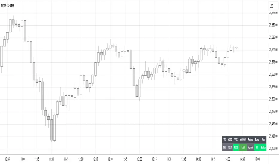
Smart Adaptive Double Patterns [The_lurker]Smart Adaptive Double Patterns
This is an advanced technical indicator that combines two of the strongest and most renowned classical price reversal patterns:
✅ Double Bottom Pattern — a bullish reversal pattern that forms after a downtrend
✅ Double Top Pattern — a bearish reversal pattern that forms after an uptrend
The indicator does not merely detect patterns — it provides a fully integrated, intelligent system that includes:
✅ Precise quality scoring for each pattern using 5 technical criteria
✅ Automatic price target calculation at three levels (Conservative, Balanced, Aggressive)
✅ Multi-layer dynamic filtering to avoid false signals
✅ Live pattern tracking from formation to target achievement or failure
✅ Comprehensive alert system covering all possible trading scenarios
🎯 Why Is This Indicator Unique?
1️⃣ High Detection Accuracy
Unlike traditional indicators that rely on simple rules, this one applies 5 strict structural conditions to confirm pattern validity:
A clear trend must precede the pattern
High symmetry between the two bottoms or two tops
No break of critical price levels during formation
Logical spacing between key points
Technical confirmation from ADX, ATR, and Volume
2️⃣ Advanced Quality Scoring System
Each pattern is scored out of 100 based on 5 weighted criteria:
Symmetry (30%): How closely the two bottoms or tops match
Trend Strength (20%): Strength of the prior trend
Volume Behavior (20%): Trading activity at critical points
Pattern Depth (15%): Vertical distance between neckline and bottom/top
Structural Integrity (15%): Full compliance with structural rules
3️⃣ Smart Target Management
Separate targets for bullish (Double Bottom) and bearish (Double Top) patterns
Separate projections for success and failure cases
Multiple options: Conservative (0.618) / Balanced (1.0) / Aggressive (1.618)
Live tracking with dynamic moving lines
4️⃣ Professional Failure Handling
Failed patterns are not ignored — they are turned into counter-trend opportunities:
Failed Double Bottom → triggers a bearish signal with downside targets
Failed Double Top → triggers a bullish signal with upside targets
Automatic color change for clear visual distinction
5️⃣ Full Customization Flexibility
Enable/disable each pattern independently
22+ adjustable settings
Unique colors for each pattern and quality level
Full bilingual support (Arabic / English)
📐 Pattern Details
🟦 Double Bottom Pattern
Sequence of points:
🔹 Point 1: Peak marking the start of a strong downtrend
🔹 Point 2 (Bottom 1): First low — first key bounce
🔹 Point 3: Intermediate high — forms the neckline (resistance)
🔹 Point 4 (Bottom 2): Second low — should closely match Bottom 1
🔹 Point 5: Breakout point — pattern confirmation
Mandatory Conditions:
✅ Clear downtrend before Point 2
✅ Bottoms 2 & 4 nearly identical (≤1.5% difference by default)
✅ Point 3 higher than both bottoms
✅ Neither bottom is broken during formation
✅ Sufficient time between points (≥10 candles by default)
✅ Success Scenario
→ Price breaks above the neckline (Point 3)
→ Point 5 is plotted at breakout candle
→ Dashed vertical line drawn from Point 5 to target
→ Horizontal dashed line tracks price toward target
→ Dashboard shows: Pattern Type | Quality | Rating | Target | Status
→ When target hits: line turns green + ✅ appears
🎯 Target Calculation
Pattern Height = Point 3 − Point 4
• Conservative: Point 3 + (Height × 0.618 × Quality Factor)
• Balanced: Point 3 + (Height × 1.0 × Quality Factor)
• Aggressive: Point 3 + (Height × 1.618 × Quality Factor)
❌ Failure Scenario
→ Price breaks below both Bottom 1 or Bottom 2 before neckline breakout
Visual Changes:
All lines turn red
Red ✖ appears at breakdown candle
Neckline stops expanding
Red dashed vertical line from breakdown point to bearish target
Red horizontal tracking line follows price
Dashboard updates to:
⚠ Failed Bottom – Bearish
→ Shows new bearish target
→ Indicates target mode for failure case
→ Status: Bearish Reversal
→ Fully red display
🟥 Double Top Pattern
Sequence of points:
🔹 Point 1: Trough marking the start of a strong uptrend
🔹 Point 2 (Top 1): First peak — first key resistance
🔹 Point 3: Intermediate low — forms the neckline (support)
🔹 Point 4 (Top 2): Second peak — should closely match Top 1
🔹 Point 5: Breakdown point — pattern confirmation
Mandatory Conditions:
✅ Clear uptrend before Point 2
✅ Tops 2 & 4 nearly identical (≤1.5% difference by default)
✅ Point 3 lower than both tops
✅ Neither top is breached during formation
✅ Sufficient time between points (≥10 candles by default)
✅ Success Scenario
→ Price breaks below the neckline (Point 3)
→ Point 5 is plotted at breakdown candle
→ Dashed vertical line drawn to target
→ Horizontal tracking line moves with price
→ Dashboard updates accordingly
→ Green line + ✅ on hit
🎯 Target Calculation
Pattern Height = Point 4 − Point 3
• Conservative: Point 3 − (Height × 0.618 × Quality Factor)
• Balanced: Point 3 − (Height × 1.0 × Quality Factor)
• Aggressive: Point 3 − (Height × 1.618 × Quality Factor)
❌ Failure Scenario
→ Price breaks above either Top 1 or Top 2 before neckline breakdown
Visual Changes:
All lines turn cyan (light blue)
Cyan ✖ appears at breakout candle
Neckline stops expanding
Cyan dashed vertical line to bullish target
Cyan horizontal tracking line follows price
Dashboard updates to:
⚠ Failed Top – Bullish
→ Shows new bullish target
→ Indicates target mode for failure case
→ Status: Bullish Reversal
→ Fully cyan display
🎯 Upside Target (after Double Top failure)
Max Top = max(Point 2, Point 4)
Height = Max Top − Point 3
• Conservative: Max Top + (Height × 0.618)
• Balanced: Max Top + (Height × 1.0)
• Aggressive: Max Top + (Height × 1.618)
📊 Quality Scoring System (0–100)
1️⃣ Symmetry (30%)
Measures price match between the two bottoms or two tops.
High score (25–30): Near-perfect symmetry → very strong pattern
Medium (15–24): Good match → reliable signal
Low (5–14): Weak symmetry → use caution
Zero: No symmetry → invalid pattern
2️⃣ Trend Strength (20%)
Uses ADX and DI indicators.
20 pts: Strong trend confirmed (e.g., ADX ≥ 20 + correct DI alignment)
10 pts: Trend filter disabled
6 pts: Weak or sideways trend
3️⃣ Volume Behavior (20%)
Declining volume on second touch is a positive sign (shows exhaustion).
15–20 pts: Clear volume drop → strong signal
10 pts: Neutral volume
6 pts: Rising volume → higher risk of continuation
4️⃣ Pattern Depth (15%)
Deeper patterns = stronger reversals.
12–15 pts: Deep → high reversal power
8–11 pts: Medium → acceptable
<8 pts: Shallow → weak signal
5️⃣ Structural Integrity (15%)
Checks logical structure (e.g., Point 1 > Point 3 in Double Bottom).
12–15 pts: Ideal structure
8–11 pts: Minor flaws
<8 pts: Poor setup
📈 Final Quality Rating & Colors
• 85–100 → ⭐ Excellent
→ Double Bottom: Cyan #00BCD4
→ Double Top: Light Red #FF5252
• 75–84 → ✨ Very Good
• 65–74 → ✓ Good
• 60–64 → ○ Acceptable
→ All use Amber #FFC107
• <60 → ❌ Rejected (not shown)
→ Gray #9E9E9E
🔧 Dynamic Filters
1️⃣ ATR Filter (Volatility Check)
Rejects patterns in abnormally high volatility periods.
→ If current ATR > 1.8 × 50-period ATR MA → pattern rejected
✅ Recommended for crypto, small caps
❌ Optional for calm markets (gold, bonds)
2️⃣ ADX Filter (Trend Confirmation)
Ensures a real trend exists before the pattern.
→ If ADX < 14 (70% of default 20) → pattern rejected
✅ Strongly recommended (keep ON)
3️⃣ Volume Filter (Behavior Validation)
Not used to reject patterns, but strongly affects quality score.
✅ Best for liquid markets (Forex majors, large stocks)
❌ Optional for illiquid assets
⚙️ Key Settings Explained
🔘 General Settings
• Language: Arabic / English
• Show Previous Patterns: Yes / No
→ “No” keeps chart clean; “Yes” for historical review
🔘 Pattern Selection
• Enable Double Bottom: ✅ / ❌
• Enable Double Top: ✅ / ❌
→ Use combinations:
✅✅ → Full reversal scanning
✅❌ → Long setups only
❌✅ → Short setups only
❌❌ → Indicator OFF
🔘 Detection Parameters
• Pivots Left (1–20): Higher = more reliable, fewer patterns
• Pivots Right (1–20): Lower = faster signals
• Min Width (5–100): Min candles between Bottom/Top 1 & 2
• Tolerance % (0.1%–5%): Max allowed price difference
• Min Arm (5–50): Min candles between pivot & neckline
• Min Trend (5–50): Min candles in prior trend
• Trend Lookback (50–500): How far back to detect trend start
• Extension Multiplier (1.0–5.0): How long to wait for breakout
🔘 Quality Settings
• Min Quality Score (0–100):
→ Conservative: 75–85
→ Balanced: 60–70
→ Flexible: 50–55
• Custom Weights: Adjust based on market (e.g., increase Volume weight in Forex)
🔘 Target Settings
• Bottom Bullish Target: Conservative / Balanced / Aggressive
• Bottom Bearish Target: (used on failure)
• Top Bearish Target: Conservative / Balanced / Aggressive
• Top Bullish Target: (used on failure)
🔘 Visual Settings
• Label Size: Small / Normal / Large / Huge
• Pattern Colors: Fully customizable
• Table: Show/Hide + Size (Small/Normal/Large) + Position (Top-Right / Top-Left / Bottom-Right / Bottom-Left)
• Fill Transparency: 70%–95% (default: 85%)
🔔 Alert System (8 Independent Alerts)
📌 Double Bottom Alerts
Bullish Breakout → “Double Bottom Breakout – Bullish!”
Bullish Target Hit → “Bullish Target Achieved!”
Failure (Bearish) → “Double Bottom Failed – Bearish!”
Bearish Target Hit → “Bearish Target Achieved (Failure)!”
📌 Double Top Alerts
Bearish Breakdown → “Double Top Breakdown – Bearish!”
Bearish Target Hit → “Bearish Target Achieved!”
Failure (Bullish) → “Double Top Failed – Bullish!”
Bullish Target Hit → “Bullish Target Achieved (Failure)!”
Each alert can be enabled/disabled independently and supports pop-ups, emails, or webhooks.
⚠️ Disclaimer:
This indicator is for educational and analytical purposes only. It does not constitute financial, investment, or trading advice. Use it in conjunction with your own strategy and risk management. Neither TradingView nor the developer is liable for any financial decisions or losses.

CHPY vs Semiconductor Sector Comparison//@version=5
indicator("CHPY vs Semiconductor Sector Comparison", overlay=false, timeframe="W")
// CHPY
chpy = request.security("CHPY", "W", close)
plot((chpy/chpy -1)*100, color=color.new(color.blue,0), title="CHPY")
// SOXX (Semiconductor Index ETF)
soxx = request.security("SOXX", "W", close)
plot((soxx/soxx -1)*100, color=color.new(color.red,0), title="SOXX")
// SMH (Semiconductor ETF)
smh = request.security("SMH", "W", close)
plot((smh/smh -1)*100, color=color.new(color.green,0), title="SMH")
// NVDA
nvda = request.security("NVDA", "W", close)
plot((nvda/nvda -1)*100, color=color.new(color.orange,0), title="NVDA")
// AVGO
avgo = request.security("AVGO", "W", close)
plot((avgo/avgo -1)*100, color=color.new(color.purple,0), title="AVGO")

Fat Tony's Composite Momentum Histogram (v01)# Fat Tony's Composite Momentum Histogram
## What It Does
This indicator combines four momentum oscillators into a single composite signal that ranges approximately from -100 to +100. It identifies potential overbought and oversold conditions while weighting signals by volume activity to filter out weak moves.
The histogram shows momentum strength with color-coded bars:
- **Red bars** indicate extreme overbought conditions (above +100)
- **Green bars** indicate extreme oversold conditions (below -100)
- **Blue bars** show positive momentum in normal range
- **Orange bars** show negative momentum in normal range
## Core Components
The indicator blends these four momentum measures:
1. **Williams %R** - Measures where price closed relative to the high-low range
2. **Stochastic %K** - Compares closing price to the recent price range
3. **MACD Histogram** - Shows momentum changes via moving average convergence/divergence
4. **ROC (Rate of Change)** - Measures percentage price change, normalized by volatility
Each component is scaled to a -50 to +50 range, then averaged together. The MACD component uses adaptive scaling based on its historical volatility to remain relevant across different market conditions.
## Volume Weighting
The indicator amplifies signals when volume is elevated and dampens them when volume is low. It uses a logarithmic scaling approach to smooth extreme volume spikes. There's also a minimum volume filter that prevents signals from triggering during very low-volume periods.
## Settings Explained
**Momentum Settings:**
- **Length (14)** - Lookback period for Williams %R and Stochastic calculations
- **MACD Fast/Slow/Signal (12/26/9)** - Standard MACD parameters
- **ROC Length (10)** - Lookback for rate of change calculation
- **MACD StDev Length (200)** - Historical window for normalizing MACD values
**Levels:**
- **Overbought Level (+100)** - Threshold for extreme upside momentum
- **Oversold Level (-100)** - Threshold for extreme downside momentum
**Volume Settings:**
- **Enable Volume Weighting** - Toggle volume amplification on/off
- **Volume Sensitivity (1.5)** - Controls how much volume impacts the signal (higher = stronger impact)
- **Min Avg Volume (50,000)** - Filters out signals when 5-bar average volume is too low
**Components:**
- **Include ROC Component** - Toggle to add/remove ROC from the calculation
- **Enable Trend Filter** - Only allows signals aligned with the 200-period EMA trend
- **Show Component Plots** - Displays individual oscillator values for tuning purposes
## Trading Signals
**Entry Signals:**
- **Long (green triangle)** - Composite crosses above the oversold level with adequate volume
- **Short (red triangle)** - Composite crosses below the overbought level with adequate volume
**Exit Signals (when trend filter enabled):**
- **Long Exit** - Composite crosses below zero from positive territory
- **Short Exit** - Composite crosses above zero from negative territory
The indicator also provides alert conditions for automated notifications on these signal events.

Trend & Strength Detector TSDTrend Strength Detector (TSD)
*Objective Trend Quality Measurement for Educational Market Analysis*
Note: This mathematical framework is a proprietary quantitative model developed by Ario Pinelab, inspired by classical EMA, ADX, RSI and MACD principles, yet not documented in any public technical or academic publication.
## 🎯 Purpose & Design Philosophy
The ** Trend Strength Detector- TSD ** is an educational research tool that provides **quantitative measurement of trend quality** through two independent scoring systems (0-100 scale). It answers the analytical question: *"How strong and aligned is the current market trend environment?"*
This indicator is designed with a **modular, complementary approach** to work alongside various analysis methodologies, particularly pattern-based recognition systems.
## 🔗 Complementary Research Framework
### Designed to Work With Pattern Detection Systems
This indicator provides **environmental context measurement** that complements qualitative pattern recognition tools. It works particularly well alongside systems like:
- **RMBS Smart Detector - Multi-Factor Momentum System**
- Traditional chart pattern analyzers
- Any momentum-based pattern identification tools
🔍 **To find RMBS Smart Detector:**
- Search in TradingView Indicators Library: `" RMBS Smart Detector - Multi-Factor Momentum System"`
- Look for: *Multi-Factor Momentum System*
- By author: ` `
### Why This Complementary Approach?
**Trend Quality Measurement** (TSD - this tool) provides:
- ✅ Structural trend alignment (0-100 score)
- ✅ Momentum intensity levels (0-100 score)
- ✅ Environment classification (Strong/Moderate/Weak)
- 📌 **Answers:** *"HOW STRONG is the underlying trend environment?"*
### Educational Research Value
When used together in a research context, these tools enable systematic study of questions like:
- How do reversal patterns behave when Strength Score is above 70 vs below 30?
- Do continuation patterns in weakening environments (declining scores) show different characteristics?
- What is the correlation between high Alignment Scores and pattern "success rates"?
- Can environment classification help identify genuine trend initiation vs false starts?
⚠️ **Important Note:** Both tools are **independent and work standalone**. TSD provides value whether used alone or with other analysis methods. The relationship with RMBS (or any pattern tool) is **complementary for research purposes**, not dependent.
---
###Mathematical Foundation
##TSA Formula: scoring method developed by Ario
-Trend Model (0 – 100)
TAS = EMA Alignment (0–40) + Price Position (0–30) + Trend Consistency (0–30)
EMA Alignment checks EMA_fast vs EMA_slow vs EMA_trend structure.
Price Position evaluates if Close is above/below all EMAs.
Consistency = 3 × max(bullish,bearish bars within 10 candles).
-Strength Model (0 – 100)
Strength = ADX (0–50) + EMA Slope (0–25) + RSI (0–15) + MACD (0–10)
ADX measures trend energy; Slope shows EMA momentum %;
RSI assesses zone positioning; MACD confirms directional agreement.
Note: This formula represents a proprietary quantitative model by Ario_Pinelab, inspired by classical technical concepts but not published in any external reference.________________________________________
📊 Environment Classification
Based on Total Strength Score:
🟢 Strong Environment: Score ≥ 60
→ Well-defined momentum, clear directional bias
🟡 Moderate Environment: 40 ≤ Score < 60
→ Mixed signals, transitional conditions
🔴 Weak Environment: Score < 40
→ Ranging, choppy, low conviction movement
Color Coding:
• Green background: Strong (≥60)
• Yellow background: Moderate (40-59)
• Red background: Weak (<40)
________________________________________
📈 Visual Components
Main Chart Display
Score Labels (Top-Right Corner):
┌─────────────────────────────────┐
│ 📊 Alignment: 75 | Strength: 82 │
│ Environment: Strong 🟢 │
└─────────────────────────────────┘
Color-Coded Background:
• Environment strength visually indicated via background color
• Helps quick identification of market regime
• Customizable transparency (default: 90%)
Reference Lines:
• Dotted line at 60: Strong/Moderate threshold
• Dotted line at 40: Moderate/Weak threshold
• Mid-line at 50: Neutral reference
________________________________________
🔧 Customization Settings
Input Parameters
The best setting is the default mode.
🚫 Important Disclaimers & Limitations
What This Indicator IS:
✅ Educational measurement tool for trend quality research
✅ Quantitative assessment of current market environment
✅ Complementary analysis tool for pattern-based systems
✅ Historical data analyzer for systematic study
✅ Multi-factor scoring system based on technical calculations
What This Indicator IS NOT:
❌ NOT a trading system or signal generator
❌ NOT financial advice or trade recommendations
❌ NOT predictive of future price movements
❌ NOT a guarantee of pattern success/failure
❌ NOT a substitute for comprehensive risk management
________________________________________
Known Limitations
1. Lagging Nature:
⚠️ All components (EMA, ADX, RSI, MACD) are calculated
from historical price data
→ Scores reflect CURRENT and RECENT conditions
→ Cannot predict sudden reversals or black swan events
→ Trend measurements lag actual price turning points
2. Whipsaw Risk:
⚠️ In choppy/ranging markets, scores may fluctuate rapidly
→ Moderate zone (40-60) can see frequent transitions
→ Low timeframes more susceptible to noise
→ Consider higher timeframes for stable measurements
3. Component Conflicts:
⚠️ Individual components may disagree
→ Example: Strong ADX but weak RSI alignment
→ Scores average these conflicts (may hide nuance)
→ Check individual components for deeper insight
4. Not Predictive:
⚠️ High scores do NOT guarantee continuation
⚠️ Low scores do NOT guarantee reversal
→ Measurement ≠ Prediction
→ Use for CONTEXT, not SIGNALS
→ Combine with comprehensive analysis
________________________________________
Risk Acknowledgments
Market Risk:
• All trading involves substantial risk of loss
• Past performance (even systematic studies) does not guarantee future results
• No indicator, system, or methodology can eliminate market risk
Measurement Limitations:
• Scores are mathematical calculations, not market predictions
• Environmental classification is descriptive, not prescriptive
• Strong measurements can deteriorate rapidly without warning
Educational Purpose:
• This tool is designed for LEARNING about market structure
• Not designed, tested, or validated as a standalone trading system
• Any trading decisions are user’s sole responsibility
No Warranty:
• Indicator provided “as-is” for educational purposes
• No guarantee of accuracy, reliability, or profitability
• Users must verify calculations and apply critical thinking
Open Source
Full Pine Script code available for educational study and modification. Feedback and improvement suggestions welcome.
“All logic is presented for research and educational visualization.”
---
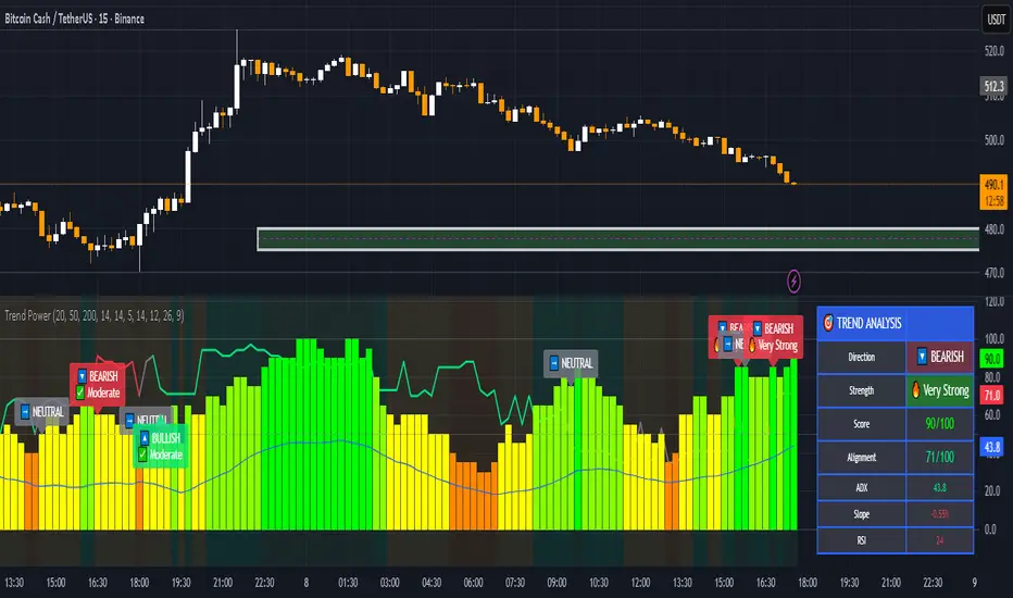
Market Structure Trailing Stop MTF [Inspired by LuxAlgo]# Market Structure Trailing Stop MTF
**OPEN-SOURCE SCRIPT**
*208k+ views on original · Modified for MTF Support*
This indicator is a direct adaptation of the renowned **Market Structure Trailing Stop** by **LuxAlgo** (original script: [Market Structure Trailing Stop ]()). The core logic remains untouched, providing dynamic trailing stops based on market structure breaks (CHoCH/BOS). The **only modification** is the addition of **Multi-Timeframe (MTF) support**, allowing users to apply the trailing stops and structures from **higher timeframes (HTF)** directly on their current chart. This enhances usability for traders analyzing cross-timeframe confluence without switching charts.
**Special thanks to LuxAlgo** for releasing this powerful open-source tool under CC BY-NC-SA 4.0. Your contributions to the TradingView community have inspired countless traders—grateful for the solid foundation!
## 🔶 How the Script Works: A Deep Dive
At its heart, this indicator detects **market structure shifts** (bullish or bearish breaks of swing highs/lows) and uses them to generate **adaptive trailing stops**. These stops trail the price while protecting profits and acting as dynamic support/resistance levels. The MTF enhancement pulls this logic from user-specified higher timeframes, overlaying HTF structures and stops on the lower timeframe chart for seamless multi-timeframe analysis.
### Core Logic (Unchanged from LuxAlgo's Original)
1. **Pivot Detection**:
- Uses `ta.pivothigh()` and `ta.pivotlow()` with a user-defined lookback (`length`) to identify swing highs (PH) and lows (PL).
- Coordinates (price `y` and bar index/time `x`) are stored in persistent variables (`var`) for tracking recent pivots.
2. **Market Structure Detection**:
- **Bullish Structure (BOS/CHoCH)**: Triggers when `close > recent PH` (break above swing high).
- If `resetOn = 'CHoCH'`, resets only on major shifts (Change of Character); otherwise, on all breaks.
- Sets trend state `os = 1` (bullish) and highlights the break with a horizontal line (dashed for CHoCH, dotted for BOS).
- Initializes trailing stop at the local minimum (lowest low since the pivot) using a backward loop: `btm = math.min(low , btm)`.
- **Bearish Structure**: Triggers when `close < recent PL`, mirroring the bullish logic (`os = -1`, local maximum for stop).
- Structure state `ms` tracks the break type (1 for bull, -1 for bear, 0 neutral), resetting based on user settings.
3. **Trailing Stop Calculation**:
- Tracks **trailing max/min**:
- On new bull structure: Reset `max = close`.
- On new bear: Reset `min = close`.
- Otherwise: `max = math.max(close, max)` / `min = math.min(close, min)`.
- **Stop Adjustment** (the "trailing" magic):
- On fresh structure: `ts = btm` (bull) or `top` (bear).
- In ongoing trend: Increment/decrement by a percentage of the max/min change:
- Bull: `ts += (max - max ) * (incr / 100)`
- Bear: `ts += (min - min ) * (incr / 100)`
- This creates a **ratcheting effect**: Stops move favorably with the trend but never against it, converging toward price at a controlled rate.
- **Visuals**:
- Plots `ts` line colored by trend (teal for bull, red for bear).
- Fills area between `close` and `ts` (orange on retracements).
- Draws structure lines from pivot to break point.
4. **Edge Cases**:
- Variables like `ph_cross`/`pl_cross` prevent multiple triggers on the same pivot.
- Neutral state (`ms = 0`) preserves prior `max/min` until a new structure.
### MTF Enhancement (Our Addition)
- **request.security() Integration**:
- Wraps the entire core function `f()` in a security call for each timeframe (`tf1`, `tf2`).
- Returns HTF values (e.g., `ts1`, `os1`, structure times/prices) to the chart's context.
- Uses `lookahead=barmerge.lookahead_off` for accurate historical repainting-free data.
- Structures are drawn using `xloc.bar_time` to align HTF lines precisely on the LTF chart.
- **Multi-Output Handling**:
- Separate plots/fills/lines for each TF (e.g., `plot_ts1`, `plot_ts2`).
- Colors and toggles per TF to distinguish HTF1 (e.g., teal/red) from HTF2 (e.g., blue/maroon).
- **Benefits**: Spot HTF bias on LTF entries, e.g., enter longs only if both TF1 (1H) and TF2 (4H) show bullish `os=1`.
This keeps the script lightweight—**no repainting, max 500 lines**, and fully compatible with LuxAlgo's original behavior when TFs are set to the chart's timeframe.
## 🔶 SETTINGS
### Core Parameters
- **Pivot Lookback** (`length = 14`): Bars left/right for pivot detection. Higher = smoother structures, fewer signals; lower = more noise.
- **Increment Factor %** (`incr = 100`): Speed of stop convergence (0-∞). 100% = full ratchet (mirrors max/min exactly); <100% = slower trail, reduces whipsaws.
- **Reset Stop On** (`'CHoCH'`): `'CHoCH'` = Reset only on major reversals (dashed lines); `'All'` = Reset on every BOS/CHoCH (tighter stops).
### MTF Support
- **Timeframe 1** (`tf1 = ""`): HTF for first set (e.g., "1H"). Empty = current chart.
- **Timeframe 2** (`tf2 = ""`): Second HTF (e.g., "4H"). Enables dual confluence.
### Display Toggles
- **Show Structures** (`true`): Draws horizontal lines for breaks (per TF colors).
- **Show Trailing Stop TF1/TF2** (`true`): Plots the stop line.
- **Show Fill TF1/TF2** (`true`): Area fill between close and stop.
### Candle Coloring (Optional)
- **Color Candles** (`false`): Enables custom `plotcandle` for body/wick/border.
- **Candle Color Based On TF** (`"None"`): `"TF1"`, `"TF2"`, or none. Colors bull trend green, bear red.
- **Candle Colors**: Separate inputs for bull/bear body, wick, border (e.g., solid green body, transparent wick).
### Alerts
- **Enable MS Break Alerts** (`false`): Notifies on structure breaks (bull/bear per TF) **only on bar close** (`barstate.isconfirmed` + `alert.freq_once_per_bar_close`).
- **Enable Stop Hit Alerts** (`false`): Triggers on stop breaches (long/short per TF), using `ta.crossunder/crossover`.
### Colors
- **TF1 Colors**: Bullish (teal), Bearish (red), Retracement (orange).
- **TF2 Colors**: Bullish (blue), Bearish (maroon), Retracement (orange).
- **Area Transparency** (`80`): Fill opacity (0-100).
## 🔶 USAGE
Trailing stops shine in **trend-following strategies**:
- **Entries**: Use structure breaks as signals (e.g., long on bullish BOS from HTF1).
- **Exits**: Trail stops for profit-locking; alert on hits for automation.
- **Confluence**: Overlay HTF1 (e.g., 1H) for bias, HTF2 (e.g., Daily) for major levels—enter LTF only on alignment.
- **Risk Management**: Lower `incr` avoids early stops in chop; reset on `'All'` for aggressive trailing.
! (i.imgur.com)
*HTF1 shows bullish structure (teal line), trailing stop ratchets up—long entry confirmed on LTF pullback.*
! (i.imgur.com)
*TF1 (blue) bearish, TF2 (red) neutral—avoid shorts until alignment.*
! (i.imgur.com)
*Colored based on TF1 trend: Green bodies on bull `os=1`.*
Pro Tip: Test on demo—pair with LuxAlgo's other tools like Smart Money Concepts for full structure ecosystem.
## 🔶 DETAILS: Mathematical Breakdown
On bullish break:
- Local min: `btm = ta.lowest(n - ph_x)` (optimized loop equivalent).
- Stop init: `ts = btm`.
- Update: `Δmax = max - max `, `ts_new = ts + Δmax * (incr/100)`.
Bearish mirrors with `Δmin` (negative, so decrements `ts`).
In MTF: HTF `time` aligns lines via `line.new(htf_time, level, current_time, level, xloc.bar_time)`.
No logs/math libs needed—pure Pine v5 efficiency.
## Disclaimer
This is for educational purposes. Not financial advice. Backtest thoroughly. Original by LuxAlgo—modify at your risk. See TradingView's (www.tradingview.com). Licensed under CC BY-NC-SA 4.0 (attribution to LuxAlgo required).

[AS] MACD-v & Hist [Alex Spiroglou | S.M.A.R.T. TRADER SYSTEMS] MACD-v & MACD-v Histogram
=======================================
Volatility Normalised Momentum 📈
Twice Awarded Indicator 🏆
=======================================
=======================================
✅ 1. INTRODUCTION TO THE MACD-v ✅
=======================================
I created the MACD-v in 2015,
as a way to deal with the limitations
of well known indicators like the Stochastic, RSI, MACD.
I decided to publicly share a very small part of my research
in the form of a research paper I wrote in 2022,
titled "MACD-v: Volatility Normalised Momentum".
That paper was awarded twice:
1. The "Charles H. Dow" Award (2022),
for outstanding research in Technical Analysis,
by the Chartered Market Technicians Association (CMTA)
2. The "Founders" Award (2022),
for advances in Active Investment Management,
by the National Association of Active Investment Managers (NAAIM)
=======================================
===================================================
❌ 2. WHY CREATE THE MACD-v ?
THE LIMITATIONS OF CONVENTIONAL MOMENTUM INDICATORS
====================================================
Technical Analysis indicators focused on momentum,
come in two general categories,
each with its own set of limitations:
(i) Range Bound Oscillators (RSI, Stochastics, etc)
These usually have a scaling of 0-100,
and thus have the advantage of having normalised readings,
that are comparable across time and securities.
However they have the following limitations (among others):
1. Skewing effect of steep trends
2. Indicator values do not adjust with and reflect true momentum
(indicator values are capped to 100)
(ii) Unbound Oscillators (MACD, RoC, etc)
These are boundless indicators,
and can expand with the market,
without being limited by a 0-100 scaling,
and thus have the advantage of really measuring momentum.
They have the main following limitations (among others):
1. Subjectivity of overbought / oversold levels
2. Not comparable across time
3. Not comparable across securities
=======================================
=======================================
💡 3. THE SOLUTION TO SOLVE THESE LIMITATIONS
=======================================
In order to deal with these limitations,
I decided to create an indicator,
that would be the "Best of two worlds".
A unique & hybrid indicator,
that would have objective normalised readings
(similar to Range Bound Oscillators - RSI)
but would also be able to have no upper/lower boundaries
(similar to Unbound Oscillators - MACD).
This would be achieved by "normalising" a boundless oscillator (MACD)
=======================================
==================================================
⛔ 4. DEEP DIVE INTO THE 5 LIMITATIONS OF THE MACD
==================================================
A Bloomberg study found that the MACD
is the most popular indicator after the RSI,
but the MACD has 5 BIG limitations.
Limitation 1: MACD values are not comparable across Time
The raw MACD values shift
as the underlying security's absolute value changes across time,
making historical comparisons obsolete
e.g S&P 500 maximum MACD was 1.56 in 1957-1971,
but reached 86.31 in 2019-2021 - not indicating 55x stronger momentum,
but simply different price levels.
Limitation 2: MACD values are not comparable across Assets
Traditional MACD cannot compare momentum between different assets.
S&P 500 MACD of 65 versus EUR/USD MACD of -0.5
reflects absolute price differences, not momentum differences
Limitation 3: MACD values cannot be Systematically Classified
Due to limitations #1 & #2, it is not possible to create
a momentum level classification scale
where one can define "fast", "slow", "overbought", "oversold" momentum
making systematic analysis impossible
Limitation 4: MACD Signal Line gives false crossovers in low-momentum ranges
In range-bound, low momentum environments,
most of the MACD signal line crossovers are false (noise)
Since there is no objective momentum classification system (limitation #3),
it is not possible to filter these signals out,
by avoiding them when momentum is low
Limitation 5: MACD Signal Line gives late crossovers in high momentum regimes.
Signal lag in strong trends not good at timing the turning point
— In high-momentum moves, MACD crossovers may come late.
Since there is no objective momentum classification system (limitation #3),
it is not possible to filter these signals out,
by avoiding them when momentum is high
===================================================================
===================================================================
🏆 5. MACD-v : THE SOLUTION TO THE LIMITATIONS OF THE MACD , RSI, etc
====================================================================
MACD-v is a volatility normalised momentum indicator.
It remedies these 5 limitations of the classic MACD,
while creating a tool with unique properties.
Formula: × 100
MACD-V enhances the classic MACD by normalizing for volatility,
transforming price-dependent readings into standardized momentum values.
This resolves key limitations of traditional MACD and adds significant analytical power.
Core Advantages of MACD-V
Advantage 1: Time-Based Stability
MACD-V values are consistent and comparable over time.
A reading of 100 has the same meaning today as it did in the past
(unlike traditional MACD which is influenced by changes in price and volatility over time)
Advantage 2: Cross-Market Comparability
MACD-V provides universal scaling.
Readings (e.g., ±50) apply consistently across all asset classes—stocks,
bonds, commodities, or currencies,
allowing traders to compare momentum across markets reliably.
Advantage 3: Objective Momentum Classification
MACD-V includes a defined 5-range momentum lifecycle
with standardized thresholds (e.g., -150 to +150).
This offers an objective framework for analyzing market conditions
and supports integration with broader models.
Advantage 4: False Signal Reduction in Low-Momentum Regimes
MACD-V introduces a "neutral zone" (typically -50 to +50)
to filter out these low-probability signals.
Advantage 5: Improved Signal Timing in High-Momentum Regimes
MACD-V identifies extremely strong trends,
allowing for more precise entry and exit points.
Advantage 6: Trend-Adaptive Scaling
Unlike bounded oscillators like RSI or Stochastic,
MACD-V dynamically expands with trend strength,
providing clearer momentum insights without artificial limits.
Advantage 7: Enhanced Divergence Detection
MACD-V offers more reliable divergence signals
by avoiding distortion at extreme levels,
a common flaw in bounded indicators (RSI, etc)
====================================================================
=======================================
⚒️ 5. HOW TO USE THE MACD-v: 7 CORE PATTERNS
HOW TO USE THE MACD-v Histogram: 2 CORE PATTERNS
=======================================
>>>>>> BASIC USE (RANGE RULES) <<<<<<
The MACD-v has 7 Core Patterns (Ranges) :
1. Risk Range (Overbought)
Condition: MACD-V > Signal Line and MACD-V > +150
Interpretation: Extremely strong bullish momentum—potential exhaustion or reversal zone.
2. Retracing
Condition: MACD-V < Signal Line and MACD-V > -50
Interpretation: Mild pullback within a bullish trend.
3. Rundown
Condition: MACD-V < Signal Line and -50 > MACD-V > -150
Interpretation: Momentum is weakening—bearish pressure building.
4. Risk Range (Oversold)
Condition: MACD-V < Signal Line and MACD-V < -150
Interpretation: Extreme bearish momentum—potential for reversal or capitulation.
5. Rebounding
Condition: MACD-V > Signal Line and MACD-V > -150
Interpretation: Bullish recovery from oversold or weak conditions.
6. Rallying
Condition: MACD-V > Signal Line and MACD-V > +50
Interpretation: Strengthening bullish trend—momentum accelerating.
7. Ranging (Neutral Zone)
Condition: MACD-V remains between -50 and +50 for 20+ bars
Interpretation: Sideways market—low conviction and momentum.
The MACD-v Histogram has 2 Core Patterns (Ranges) :
1. Risk (Overbought)
Condition: Histogram > +40
Interpretation: Short-term bullish momentum is stretched—possible overextension or reversal risk.
2. Risk (Oversold)
Condition: Histogram < -40
Interpretation: Short-term bearish momentum is stretched—potential for rebound or reversal.
=======================================
=======================================
📈 6. ADVANCED PATTERNS WITH MACD-v
=======================================
Thanks to its volatility normalization,
the MACD-V framework enables the development
of a wide range of advanced pattern recognition setups,
trading signals, and strategic models.
These patterns go beyond basic crossovers,
offering deeper insight into momentum structure,
regime shifts, and high-probability trade setups.
These are not part of this script
=======================================
===========================================================
⚙️ 7. FUNCTIONALITY - HOW TO ADD THE INDICATORS TO YOUR CHART
===========================================================
The script allows you to see :
1. MACD-v
The indicator with the ranges (150,50,0,-50,-150)
and colour coded according to its 7 basic patterns
2. MACD-v Histogram
The indicator The indicator with the ranges (40,0,-40)
and colour coded according to its 2 basic ranges / patterns
3. MACD-v Heatmap
You can see the MACD-v in a Multiple Timeframe basis,
using a colour-coded Heatmap
Note that lowest timeframe in the heatmap must be the one on the chart
i.e. if you see the daily chart, then the Heatmap will be Daily, Weekly, Monthly
4. MACD-v Dashboard
You can see the MACD-v for 7 markets,
in a multiple timeframe basis
=======================================
=======================================
🤝 CONTRIBUTIONS 🤝
=======================================
I would like to thank the following people:
1. Mike Christensen for coding the indicator
@TradersPostInc, @Mik3Christ3ns3n,
2. @Indicator-Jones For allowing me to use his Scanner
3. @Daveatt For allowing me to use his heatmap
=======================================
=======================================
⚠️ LEGAL - Usage and Attribution Notice ⚠️
=======================================
Use of this Script is permitted
for personal or non-commercial purposes,
including implementation by coders and TradingView users.
However, any form of paid redistribution,
resale, or commercial exploitation is strictly prohibited.
Proper attribution to the original author is expected and appreciated,
in order to acknowledge the source
and maintain the integrity of the original work.
Failure to comply with these terms,
or to take corrective action within 48 hours of notification,
will result in a formal report to TradingView’s moderation team,
and will actively pursue account suspension and removal of the infringing script(s).
Continued violations may result in further legal action, as deemed necessary.
=======================================
=======================================
⚠️ DISCLAIMER ⚠️
=======================================
This indicator is For Educational Purposes Only (F.E.P.O.).
I am just Teaching by Example (T.B.E.)
It does not constitute investment advice.
There are no guarantees in trading - except one.
You will have losses in trading.
I can guarantee you that with 100% certainty.
The author is not responsible for any financial losses
or trading decisions made based on this indicator. 🙏
Always perform your own analysis and use proper risk management. 🛡️
=======================================

Ultimate Oscillator (ULTOSC)The Ultimate Oscillator (ULTOSC) is a technical momentum indicator developed by Larry Williams that combines three different time periods to reduce the volatility and false signals common in single-period oscillators. By using a weighted average of three Stochastic-like calculations across short, medium, and long-term periods, the Ultimate Oscillator provides a more comprehensive view of market momentum while maintaining sensitivity to price changes.
The indicator addresses the common problem of oscillators being either too sensitive (generating many false signals) or too slow (missing opportunities). By incorporating multiple timeframes with decreasing weights for longer periods, ULTOSC attempts to capture both short-term momentum shifts and longer-term trend strength, making it particularly valuable for identifying divergences and potential reversal points.
## Core Concepts
* **Multi-timeframe analysis:** Combines three different periods (typically 7, 14, 28) to capture various momentum cycles
* **Weighted averaging:** Assigns higher weights to shorter periods for responsiveness while including longer periods for stability
* **Buying pressure focus:** Measures the relationship between closing price and the true range rather than just high-low range
* **Divergence detection:** Particularly effective at identifying momentum divergences that precede price reversals
* **Normalized scale:** Oscillates between 0 and 100, with clear overbought/oversold levels
## Common Settings and Parameters
| Parameter | Default | Function | When to Adjust |
|-----------|---------|----------|---------------|
| Fast Period | 7 | Short-term momentum calculation | Lower (5-6) for more sensitivity, higher (9-12) for smoother signals |
| Medium Period | 14 | Medium-term momentum calculation | Adjust based on typical swing duration in the market |
| Slow Period | 28 | Long-term momentum calculation | Higher values (35-42) for longer-term position trading |
| Fast Weight | 4.0 | Weight applied to fast period | Higher weight increases short-term sensitivity |
| Medium Weight | 2.0 | Weight applied to medium period | Adjust to balance medium-term influence |
| Slow Weight | 1.0 | Weight applied to slow period | Usually kept at 1.0 as the baseline weight |
**Pro Tip:** The classic 7/14/28 periods with 4/2/1 weights work well for most markets, but consider using 5/10/20 with adjusted weights for faster markets or 14/28/56 for longer-term analysis.
## Calculation and Mathematical Foundation
**Simplified explanation:**
The Ultimate Oscillator calculates three separate "buying pressure" ratios using different time periods, then combines them using weighted averaging. Buying pressure is defined as the close minus the true low, divided by the true range.
**Technical formula:**
```
BP = Close - Min(Low, Previous Close)
TR = Max(High, Previous Close) - Min(Low, Previous Close)
BP_Sum_Fast = Sum(BP, Fast Period)
TR_Sum_Fast = Sum(TR, Fast Period)
Raw_Fast = 100 × (BP_Sum_Fast / TR_Sum_Fast)
BP_Sum_Medium = Sum(BP, Medium Period)
TR_Sum_Medium = Sum(TR, Medium Period)
Raw_Medium = 100 × (BP_Sum_Medium / TR_Sum_Medium)
BP_Sum_Slow = Sum(BP, Slow Period)
TR_Sum_Slow = Sum(TR, Slow Period)
Raw_Slow = 100 × (BP_Sum_Slow / TR_Sum_Slow)
ULTOSC = 100 × / (Fast_Weight + Medium_Weight + Slow_Weight)
```
Where:
- BP = Buying Pressure
- TR = True Range
- Fast Period = 7, Medium Period = 14, Slow Period = 28 (defaults)
- Fast Weight = 4, Medium Weight = 2, Slow Weight = 1 (defaults)
> 🔍 **Technical Note:** The implementation uses efficient circular buffers for all three period calculations, maintaining O(1) time complexity per bar. The algorithm properly handles true range calculations including gaps and ensures accurate buying pressure measurements across all timeframes.
## Interpretation Details
ULTOSC provides several analytical perspectives:
* **Overbought/Oversold conditions:** Values above 70 suggest overbought conditions, below 30 suggest oversold conditions
* **Momentum direction:** Rising ULTOSC indicates increasing buying pressure, falling indicates increasing selling pressure
* **Divergence analysis:** Divergences between ULTOSC and price often precede significant reversals
* **Trend confirmation:** ULTOSC direction can confirm or question the prevailing price trend
* **Signal quality:** Extreme readings (>80 or <20) indicate strong momentum that may be unsustainable
* **Multiple timeframe consensus:** When all three underlying periods agree, signals are typically more reliable
## Trading Applications
**Primary Uses:**
- **Divergence trading:** Identify when momentum diverges from price for reversal signals
- **Overbought/oversold identification:** Find potential entry/exit points at extreme levels
- **Trend confirmation:** Validate breakouts and trend continuations
- **Momentum analysis:** Assess the strength of current price movements
**Advanced Strategies:**
- **Multi-divergence confirmation:** Look for divergences across multiple timeframes
- **Momentum breakouts:** Trade when ULTOSC breaks above/below key levels with volume
- **Swing trading entries:** Use oversold/overbought levels for swing position entries
- **Trend strength assessment:** Evaluate trend quality using momentum consistency
## Signal Combinations
**Strong Bullish Signals:**
- ULTOSC rises from oversold territory (<30) with positive price divergence
- ULTOSC breaks above 50 after forming a base near 30
- All three underlying periods show increasing buying pressure
**Strong Bearish Signals:**
- ULTOSC falls from overbought territory (>70) with negative price divergence
- ULTOSC breaks below 50 after forming a top near 70
- All three underlying periods show decreasing buying pressure
**Divergence Signals:**
- **Bullish divergence:** Price makes lower lows while ULTOSC makes higher lows
- **Bearish divergence:** Price makes higher highs while ULTOSC makes lower highs
- **Hidden bullish divergence:** Price makes higher lows while ULTOSC makes lower lows (trend continuation)
- **Hidden bearish divergence:** Price makes lower highs while ULTOSC makes higher highs (trend continuation)
## Comparison with Related Oscillators
| Indicator | Periods | Focus | Best Use Case |
|-----------|---------|-------|---------------|
| **Ultimate Oscillator** | 3 periods | Buying pressure | Divergence detection |
| **Stochastic** | 1-2 periods | Price position | Overbought/oversold |
| **RSI** | 1 period | Price momentum | Momentum analysis |
| **Williams %R** | 1 period | Price position | Short-term signals |
## Advanced Configurations
**Fast Trading Setup:**
- Fast: 5, Medium: 10, Slow: 20
- Weights: 4/2/1, Thresholds: 75/25
**Standard Setup:**
- Fast: 7, Medium: 14, Slow: 28
- Weights: 4/2/1, Thresholds: 70/30
**Conservative Setup:**
- Fast: 14, Medium: 28, Slow: 56
- Weights: 3/2/1, Thresholds: 65/35
**Divergence Focused:**
- Fast: 7, Medium: 14, Slow: 28
- Weights: 2/2/2, Thresholds: 70/30
## Market-Specific Adjustments
**Volatile Markets:**
- Use longer periods (10/20/40) to reduce noise
- Consider higher threshold levels (75/25)
- Focus on extreme readings for signal quality
**Trending Markets:**
- Emphasize divergence analysis over absolute levels
- Look for momentum confirmation rather than reversal signals
- Use hidden divergences for trend continuation
**Range-Bound Markets:**
- Standard overbought/oversold levels work well
- Trade reversals from extreme levels
- Combine with support/resistance analysis
## Limitations and Considerations
* **Lagging component:** Contains inherent lag due to multiple moving average calculations
* **Complex calculation:** More computationally intensive than single-period oscillators
* **Parameter sensitivity:** Performance varies significantly with different period/weight combinations
* **Market dependency:** Most effective in trending markets with clear momentum patterns
* **False divergences:** Not all divergences lead to significant price reversals
* **Whipsaw potential:** Can generate conflicting signals in choppy markets
## Best Practices
**Effective Usage:**
- Focus on divergences rather than absolute overbought/oversold levels
- Combine with trend analysis for context
- Use multiple timeframe analysis for confirmation
- Pay attention to the speed of momentum changes
**Common Mistakes:**
- Over-relying on overbought/oversold levels in strong trends
- Ignoring the underlying trend direction
- Using inappropriate period settings for the market being analyzed
- Trading every divergence without additional confirmation
**Signal Enhancement:**
- Combine with volume analysis for confirmation
- Use price action context (support/resistance levels)
- Consider market volatility when setting thresholds
- Look for convergence across multiple momentum indicators
## Historical Context and Development
The Ultimate Oscillator was developed by Larry Williams and introduced in his 1985 article "The Ultimate Oscillator" in Technical Analysis of Stocks and Commodities magazine. Williams designed it to address the limitations of single-period oscillators by:
- Reducing false signals through multi-timeframe analysis
- Maintaining sensitivity to short-term momentum changes
- Providing more reliable divergence signals
- Creating a more robust momentum measurement tool
The indicator has become a standard tool in technical analysis, particularly valued for its divergence detection capabilities and its balanced approach to momentum measurement.
## References
* Williams, L. R. (1985). The Ultimate Oscillator. Technical Analysis of Stocks and Commodities, 3(4).
* Williams, L. R. (1999). Long-Term Secrets to Short-Term Trading. Wiley Trading.

Velocity Pressure Index | AlphaNattVelocity Pressure Index (VPI) | AlphaNatt
A sophisticated momentum oscillator that combines price velocity analysis with volume pressure dynamics to identify high-probability trading opportunities.
📊 KEY FEATURES
Dual Analysis System: Merges price velocity measurement with volume pressure analysis for comprehensive market momentum assessment
Dynamic Normalization: Automatically scales values between -100 and +100 for consistent readings across all market conditions
Adaptive Zones: Self-adjusting overbought/oversold levels based on recent price history
Multi-Layer Confirmation: Combines momentum, acceleration, and crossover signals for robust trade identification
Volume-Weighted Pressure: Differentiates between bullish and bearish volume to gauge true market sentiment
📈 HOW IT WORKS
The VPI calculates price velocity using linear regression of price changes, then weights this velocity by the difference between bullish and bearish volume pressure. This creates a momentum reading that accounts for both price movement speed and the volume conviction behind it.
Signal Generation:
Price velocity is measured over the specified period
Volume is separated into bullish (close > open) and bearish (close < open) pressure
Velocity is amplified or dampened based on volume pressure differential
The resulting index is normalized to oscillate between -100 and +100
A signal line smooths the oscillator for crossover detection
🎯 TRADING SIGNALS
Long Signals (Cyan #00F1FF):
Strong Bull: VPI > Signal with positive momentum and acceleration
Crossover Bull: VPI crosses above signal while above oversold zone
Divergence: Price makes lower low while VPI makes higher low
Short Signals (Magenta #FF019A):
Strong Bear: VPI < Signal with negative momentum and deceleration
Crossover Bear: VPI crosses below signal while below overbought zone
Divergence: Price makes higher high while VPI makes lower high
⚙️ CUSTOMIZABLE PARAMETERS
Velocity Settings:
Velocity Period (14): Lookback for price velocity calculation
Pressure Period (21): Volume analysis window
Smoothing Factor (3): Final oscillator smoothing
Signal Configuration:
Signal Type: Choose between SMA, EMA, or DEMA
Signal Length (9): Signal line smoothing period
Normalization Period (50): Range calculation window
Dynamic Zones:
Zone Lookback (100): Period for adaptive overbought/oversold calculation
Percentiles: 80th/20th percentiles for dynamic zones
📐 VISUAL COMPONENTS
Main Oscillator: Color-coded line showing current momentum state
Signal Line: White line for crossover detection
Momentum Histogram: Shows velocity differential at 50% scale
Dynamic Zones: Self-adjusting overbought/oversold bands
Extreme Levels: ±50 dotted lines marking extreme conditions
Background Shading: Subtle highlighting of overbought/oversold regions
💡 USAGE TIPS
Trend Trading: Use strong bull/bear signals in trending markets for continuation entries
Range Trading: Focus on crossovers near extreme zones for reversal trades
Divergence Trading: Watch for price/oscillator divergences at market extremes
Multi-Timeframe: Combine with higher timeframe VPI for directional bias
Volume Confirmation: Stronger signals occur with aligned volume pressure
⚠️ BEST PRACTICES
The VPI works best in liquid markets with reliable volume data. For optimal results, combine with price action analysis and use appropriate risk management. The indicator is most effective during trending conditions but can identify reversals when divergences occur at extremes.
🔔 ALERTS AVAILABLE
VPI Long/Short Signals
Bullish/Bearish Crossovers
Extreme Overbought/Oversold Conditions
Version 6 | Pine Script™ | © AlphaNatt

Index of Civilization DevelopmentIndex of Civilization Development Indicator
This Pine Script (version 6) creates a custom technical indicator for TradingView, titled Index of Civilization Development. It generates a composite index by averaging normalized stock market performances from a selection of global country indices. The normalization is relative to each index's 100-period simple moving average (SMA), scaled to a percentage (100% baseline). This allows for a comparable "development" or performance metric across diverse markets, potentially highlighting trends in global economic or "civilizational" progress based on equity markets.The indicator plots as a single line in a separate pane (non-overlay) and is designed to handle up to 40 symbols to respect TradingView's request.security() call limits.Key FeaturesComposite Index Calculation: Fetches the previous bar's close (close ) and its 100-period SMA for each selected symbol.
Normalizes each: (close / SMA(100)) * 100.
Averages the valid normalizations (ignores invalid/NA data) to produce a single "Index (%)" value.
Symbol Selection Modes:Top N Countries: Selects from a predefined list of the top 50 global stock indices (by market cap/importance, e.g., SPX for USA, SHCOMP for China). Options: Top 5, 15, 25, or 50.
Democratic Countries: ~38 symbols from democracies (e.g., SPX, NI225, NIFTY; based on democracy indices ≥6/10, including flawed/parliamentary systems).
Dictatorships: ~12 symbols from authoritarian/hybrid regimes (e.g., SHCOMP, TASI, IMOEX; scores <6/10).
Customization:Line color (default: blue).
Line width (1-5, default: 2).
Line style: Solid line (default), Stepline, or Circles.
Data Handling:Uses request.security() with lookahead enabled for real-time accuracy, gaps off, and invalid symbol ignoring.
Runs calculations on every bar, with max_bars_back=2000 for historical depth.
Arrays are populated only on the first bar (barstate.isfirst) for efficiency.
Predefined Symbol Lists (Examples)Top 50: SPX (USA), SHCOMP (China), NI225 (Japan), ..., BAX (Bahrain).
Democratic: Focuses on free-market democracies like USA, Japan, UK, Canada, EU nations, Australia, etc.
Dictatorships: Authoritarian markets like China, Saudi Arabia, Russia, Turkey, etc.
Usage TipsAdd to any chart (e.g., daily/weekly timeframe) to view the composite line.
Ideal for macro analysis: Compare democratic vs. authoritarian performance, or track "top world" equity health.
Potential Limitations: Relies on TradingView's symbol availability; some exotic indices (e.g., KWSEIDX) may fail if not supported. The 40-symbol cap prevents errors.
Interpretation: Values >100 indicate above-trend performance; <100 suggest underperformance relative to recent averages.
This script blends financial data with geopolitical categorization for a unique "civilization index" perspective on global markets. For modifications, ensure symbol tickers match TradingView's format.
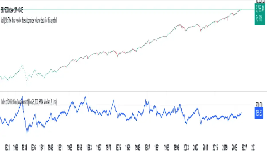
BOCS Channel Scalper Strategy - Automated Mean Reversion System# BOCS Channel Scalper Strategy - Automated Mean Reversion System
## WHAT THIS STRATEGY DOES:
This is an automated mean reversion trading strategy that identifies consolidation channels through volatility analysis and executes scalp trades when price enters entry zones near channel boundaries. Unlike breakout strategies, this system assumes price will revert to the channel mean, taking profits as price bounces back from extremes. Position sizing is fully customizable with three methods: fixed contracts, percentage of equity, or fixed dollar amount. Stop losses are placed just outside channel boundaries with take profits calculated either as fixed points or as a percentage of channel range.
## KEY DIFFERENCE FROM ORIGINAL BOCS:
**This strategy is designed for traders seeking higher trade frequency.** The original BOCS indicator trades breakouts OUTSIDE channels, waiting for price to escape consolidation before entering. This scalper version trades mean reversion INSIDE channels, entering when price reaches channel extremes and betting on a bounce back to center. The result is significantly more trading opportunities:
- **Original BOCS**: 1-3 signals per channel (only on breakout)
- **Scalper Version**: 5-15+ signals per channel (every touch of entry zones)
- **Trade Style**: Mean reversion vs trend following
- **Hold Time**: Seconds to minutes vs minutes to hours
- **Best Markets**: Ranging/choppy conditions vs trending breakouts
This makes the scalper ideal for active day traders who want continuous opportunities within consolidation zones rather than waiting for breakout confirmation. However, increased trade frequency also means higher commission costs and requires tighter risk management.
## TECHNICAL METHODOLOGY:
### Price Normalization Process:
The strategy normalizes price data to create consistent volatility measurements across different instruments and price levels. It calculates the highest high and lowest low over a user-defined lookback period (default 100 bars). Current close price is normalized using: (close - lowest_low) / (highest_high - lowest_low), producing values between 0 and 1 for standardized volatility analysis.
### Volatility Detection:
A 14-period standard deviation is applied to the normalized price series to measure price deviation from the mean. Higher standard deviation values indicate volatility expansion; lower values indicate consolidation. The strategy uses ta.highestbars() and ta.lowestbars() to identify when volatility peaks and troughs occur over the detection period (default 14 bars).
### Channel Formation Logic:
When volatility crosses from a high level to a low level (ta.crossover(upper, lower)), a consolidation phase begins. The strategy tracks the highest and lowest prices during this period, which become the channel boundaries. Minimum duration of 10+ bars is required to filter out brief volatility spikes. Channels are rendered as box objects with defined upper and lower boundaries, with colored zones indicating entry areas.
### Entry Signal Generation:
The strategy uses immediate touch-based entry logic. Entry zones are defined as a percentage from channel edges (default 20%):
- **Long Entry Zone**: Bottom 20% of channel (bottomBound + channelRange × 0.2)
- **Short Entry Zone**: Top 20% of channel (topBound - channelRange × 0.2)
Long signals trigger when candle low touches or enters the long entry zone. Short signals trigger when candle high touches or enters the short entry zone. This captures mean reversion opportunities as price reaches channel extremes.
### Cooldown Filter:
An optional cooldown period (measured in bars) prevents signal spam by enforcing minimum spacing between consecutive signals. If cooldown is set to 3 bars, no new long signal will fire until 3 bars after the previous long signal. Long and short cooldowns are tracked independently, allowing both directions to signal within the same period.
### ATR Volatility Filter:
The strategy includes a multi-timeframe ATR filter to avoid trading during low-volatility conditions. Using request.security(), it fetches ATR values from a specified timeframe (e.g., 1-minute ATR while trading on 5-minute charts). The filter compares current ATR to a user-defined minimum threshold:
- If ATR ≥ threshold: Trading enabled
- If ATR < threshold: No signals fire
This prevents entries during dead zones where mean reversion is unreliable due to insufficient price movement.
### Take Profit Calculation:
Two TP methods are available:
**Fixed Points Mode**:
- Long TP = Entry + (TP_Ticks × syminfo.mintick)
- Short TP = Entry - (TP_Ticks × syminfo.mintick)
**Channel Percentage Mode**:
- Long TP = Entry + (ChannelRange × TP_Percent)
- Short TP = Entry - (ChannelRange × TP_Percent)
Default 50% targets the channel midline, a natural mean reversion target. Larger percentages aim for opposite channel edge.
### Stop Loss Placement:
Stop losses are placed just outside the channel boundary by a user-defined tick offset:
- Long SL = ChannelBottom - (SL_Offset_Ticks × syminfo.mintick)
- Short SL = ChannelTop + (SL_Offset_Ticks × syminfo.mintick)
This logic assumes channel breaks invalidate the mean reversion thesis. If price breaks through, the range is no longer valid and position exits.
### Trade Execution Logic:
When entry conditions are met (price in zone, cooldown satisfied, ATR filter passed, no existing position):
1. Calculate entry price at zone boundary
2. Calculate TP and SL based on selected method
3. Execute strategy.entry() with calculated position size
4. Place strategy.exit() with TP limit and SL stop orders
5. Update info table with active trade details
The strategy enforces one position at a time by checking strategy.position_size == 0 before entry.
### Channel Breakout Management:
Channels are removed when price closes more than 10 ticks outside boundaries. This tolerance prevents premature channel deletion from minor breaks or wicks, allowing the mean reversion setup to persist through small boundary violations.
### Position Sizing System:
Three methods calculate position size:
**Fixed Contracts**:
- Uses exact contract quantity specified in settings
- Best for futures traders (e.g., "trade 2 NQ contracts")
**Percentage of Equity**:
- position_size = (strategy.equity × equity_pct / 100) / close
- Dynamically scales with account growth
**Cash Amount**:
- position_size = cash_amount / close
- Maintains consistent dollar exposure regardless of price
## INPUT PARAMETERS:
### Position Sizing:
- **Position Size Type**: Choose Fixed Contracts, % of Equity, or Cash Amount
- **Number of Contracts**: Fixed quantity per trade (1-1000)
- **% of Equity**: Percentage of account to allocate (1-100%)
- **Cash Amount**: Dollar value per position ($100+)
### Channel Settings:
- **Nested Channels**: Allow multiple overlapping channels vs single channel
- **Normalization Length**: Lookback for high/low calculation (1-500, default 100)
- **Box Detection Length**: Period for volatility detection (1-100, default 14)
### Scalping Settings:
- **Enable Long Scalps**: Toggle long entries on/off
- **Enable Short Scalps**: Toggle short entries on/off
- **Entry Zone % from Edge**: Size of entry zone (5-50%, default 20%)
- **SL Offset (Ticks)**: Distance beyond channel for stop (1+, default 5)
- **Cooldown Period (Bars)**: Minimum spacing between signals (0 = no cooldown)
### ATR Filter:
- **Enable ATR Filter**: Toggle volatility filter on/off
- **ATR Timeframe**: Source timeframe for ATR (1, 5, 15, 60 min, etc.)
- **ATR Length**: Smoothing period (1-100, default 14)
- **Min ATR Value**: Threshold for trade enablement (0.1+, default 10.0)
### Take Profit Settings:
- **TP Method**: Choose Fixed Points or % of Channel
- **TP Fixed (Ticks)**: Static distance in ticks (1+, default 30)
- **TP % of Channel**: Dynamic target as channel percentage (10-100%, default 50%)
### Appearance:
- **Show Entry Zones**: Toggle zone labels on channels
- **Show Info Table**: Display real-time strategy status
- **Table Position**: Corner placement (Top Left/Right, Bottom Left/Right)
- **Color Settings**: Customize long/short/TP/SL colors
## VISUAL INDICATORS:
- **Channel boxes** with semi-transparent fill showing consolidation zones
- **Colored entry zones** labeled "LONG ZONE ▲" and "SHORT ZONE ▼"
- **Entry signal arrows** below/above bars marking long/short entries
- **Active TP/SL lines** with emoji labels (⊕ Entry, 🎯 TP, 🛑 SL)
- **Info table** showing position status, channel state, last signal, entry/TP/SL prices, and ATR status
## HOW TO USE:
### For 1-3 Minute Scalping (NQ/ES):
- ATR Timeframe: "1" (1-minute)
- ATR Min Value: 10.0 (for NQ), adjust per instrument
- Entry Zone %: 20-25%
- TP Method: Fixed Points, 20-40 ticks
- SL Offset: 5-10 ticks
- Cooldown: 2-3 bars
- Position Size: 1-2 contracts
### For 5-15 Minute Day Trading:
- ATR Timeframe: "5" or match chart
- ATR Min Value: Adjust to instrument (test 8-15 for NQ)
- Entry Zone %: 20-30%
- TP Method: % of Channel, 40-60%
- SL Offset: 5-10 ticks
- Cooldown: 3-5 bars
- Position Size: Fixed contracts or 5-10% equity
### For 30-60 Minute Swing Scalping:
- ATR Timeframe: "15" or "30"
- ATR Min Value: Lower threshold for broader market
- Entry Zone %: 25-35%
- TP Method: % of Channel, 50-70%
- SL Offset: 10-15 ticks
- Cooldown: 5+ bars or disable
- Position Size: % of equity recommended
## BACKTEST CONSIDERATIONS:
- Strategy performs best in ranging, mean-reverting markets
- Strong trending markets produce more stop losses as price breaks channels
- ATR filter significantly reduces trade count but improves quality during low volatility
- Cooldown period trades signal quantity for signal quality
- Commission and slippage materially impact sub-5-minute timeframe performance
- Shorter timeframes require tighter entry zones (15-20%) to catch quick reversions
- % of Channel TP adapts better to varying channel sizes than fixed points
- Fixed contract sizing recommended for consistent risk per trade in futures
**Backtesting Parameters Used**: This strategy was developed and tested using realistic commission and slippage values to provide accurate performance expectations. Recommended settings: Commission of $1.40 per side (typical for NQ futures through discount brokers), slippage of 2 ticks to account for execution delays on fast-moving scalp entries. These values reflect real-world trading costs that active scalpers will encounter. Backtest results without proper cost simulation will significantly overstate profitability.
## COMPATIBLE MARKETS:
Works on any instrument with price data including stock indices (NQ, ES, YM, RTY), individual stocks, forex pairs (EUR/USD, GBP/USD), cryptocurrency (BTC, ETH), and commodities. Volume-based features require data feed with volume information but are optional for core functionality.
## KNOWN LIMITATIONS:
- Immediate touch entry can fire multiple times in choppy zones without adequate cooldown
- Channel deletion at 10-tick breaks may be too aggressive or lenient depending on instrument tick size
- ATR filter from lower timeframes requires higher-tier TradingView subscription (request.security limitation)
- Mean reversion logic fails in strong breakout scenarios leading to stop loss hits
- Position sizing via % of equity or cash amount calculates based on close price, may differ from actual fill price
- No partial closing capability - full position exits at TP or SL only
- Strategy does not account for gap openings or overnight holds
## RISK DISCLOSURE:
Trading involves substantial risk of loss. Past performance does not guarantee future results. This strategy is for educational purposes and backtesting only. Mean reversion strategies can experience extended drawdowns during trending markets. Stop losses may not fill at intended levels during extreme volatility or gaps. Thoroughly test on historical data and paper trade before risking real capital. Use appropriate position sizing and never risk more than you can afford to lose. Consider consulting a licensed financial advisor before making trading decisions. Automated trading systems can malfunction - monitor all live positions actively.
## ACKNOWLEDGMENT & CREDITS:
This strategy is built upon the channel detection methodology created by **AlgoAlpha** in the "Smart Money Breakout Channels" indicator. Full credit and appreciation to AlgoAlpha for pioneering the normalized volatility approach to identifying consolidation patterns. The core channel formation logic using normalized price standard deviation is AlgoAlpha's original contribution to the TradingView community.
Enhancements to the original concept include: mean reversion entry logic (vs breakout), immediate touch-based signals, multi-timeframe ATR volatility filtering, flexible position sizing (fixed/percentage/cash), cooldown period filtering, dual TP methods (fixed points vs channel percentage), automated strategy execution with exit management, and real-time position monitoring table.

BioSwarm Imprinter™BioSwarm Imprinter™ — Agent-Based Consensus for Traders
What it is
BioSwarm Imprinter™ is a non-repainting, agent-based sentiment oscillator. It fuses many short-to-medium lookback “opinions” into one 0–100 consensus line that is easy to read at a glance (50 = neutral, >55 bullish bias, <45 bearish bias). The engine borrows from swarm intelligence: many simple voters (agents) adapt their influence over time based on how well they’ve been predicting price, so the crowd gets smarter as conditions change.
Use it to:
• Detect emerging trends sooner without overreacting to noise.
• Filter mean-reversion vs continuation opportunities.
• Gate entries with a confidence score that reflects both strength and persistence of the move.
• Combine with your execution tools (VWAP/ORB/levels) as a state filter rather than a trade signal by itself.
⸻
Why it’s different
• Swarm learning: Each agent improves or decays its “fitness” depending on whether its vote matched the next bar’s direction. High-fitness agents matter more; weak agents fade.
• Multi-horizon by design: The crowd is composed of fixed, simple lookbacks spread from lenMin to lenMax. You get a blended, robust view instead of a single fragile parameter.
• Two complementary lenses: Each agent evaluates RSI-style balance (via Wilder’s RMA) and momentum (EMA deviation). You decide the weight of each.
• No repaint, no MTF pitfalls: Everything runs on the chart’s timeframe with bar-close confirmation; no request.security() or forward references.
• Actionable UI: A clean consensus line, optional regime background, confidence heat, and triangle markers when thresholds are crossed.
⸻
What you see on the chart
• Consensus line (0–100): Smoothed to your preference; color/area makes bull/bear zones obvious.
• Regime coloring (optional): Light green in bull zone, light red in bear zone; neutral otherwise.
• Confidence heat: A small gauge/number (0–100) that combines distance from neutral and recent persistence.
• Markers (optional): Triangles when consensus crosses up through your bull threshold (e.g., 55) or down through your bear threshold (e.g., 45).
• Info panel (optional): Consensus value, regime, confidence, number of agents, and basic diagnostics.
⸻
How it works (under the hood)
1. Horizon bins: The range is divided into numBins. Each bin has a fixed, simple integer length (crucial for Pine’s safety rules).
2. Per-bin features (computed every bar):
• RSI-style balance using Wilder’s RMA (not ta.rsi()), then mapped to −1…+1.
• Momentum as (close − EMA(L)) / EMA(L) (dimensionless drift).
3. Agent vote: For its assigned bin, an agent forms a weighted score: score = wRSI*RSI_like + wMOM*Momentum. A small dead-band near zero suppresses chop; votes are +1/−1/0.
4. Fitness update (bar close): If the agent’s previous vote agreed with the next bar’s direction, multiply its fitness by learnGain; otherwise by learnPain. Fitness is clamped so it never explodes or dies.
5. Consensus: Weighted average of all votes using fitness as weights → map to 0–100 and smooth with EMA.
Why it doesn’t repaint:
• No future references, no MTF resampling, fitness updates only on confirmed bars.
• All TA primitives (RMA/EMA/deltas) are computed every bar unconditionally.
⸻
Signals & confidence
• Bullish bias: consensus ≥ bullThr (e.g., 55).
• Bearish bias: consensus ≤ bearThr (e.g., 45).
• Confidence (0–100):
• Distance score: how far consensus is from 50.
• Momentum score: how strong the recent change is versus its recent average.
• Combined into a single gate; start filtering entries at ≥60 for higher quality.
Tip: For range sessions, raise thresholds (60/40) and increase smoothing; for momentum sessions, lower smoothing and keep thresholds at 55/45.
⸻
Inputs you’ll actually tune
• Agents & horizons:
• N_agents (e.g., 64–128)
• lenMin / lenMax (e.g., 6–30 intraday, 10–60 swing)
• numBins (e.g., 12–24)
• Weights & smoothing:
• wRSI vs wMOM (e.g., 0.7/0.3 for FX & indices; 0.6/0.4 for crypto)
• deadBand (0.03–0.08)
• consSmooth (3–8)
• Thresholds & hygiene:
• bullThr/bearThr (55/45 default)
• cooldownBars to avoid signal spam
⸻
Playbooks (ready-to-use)
1) Breakout / Trend continuation
• Timeframe: 15m–1h for day/swing.
• Filter: Take longs only when consensus > 55 and confidence ≥ 60.
• Execution: Use your ORB/VWAP/pullback trigger for entry. Trail with swing lows or 1.5×ATR. Exit on a close back under 50 or when a bearish signal prints.
2) Mean reversion (fade)
• When: Sideways days or low-volatility clusters.
• Setup: Increase deadBand and consSmooth.
• Signal: Bearish fades when consensus rolls over below ≈55 but stays above 50; bullish fades when it rolls up above ≈45 but stays below 50.
• Targets: The neutral zone (~50) as the first take-profit.
3) Multi-TF alignment
• Keep BioSwarm on 1H for bias, execute on 5–15m:
• Only take entries in the direction of the 1H consensus.
• Skip counter-bias scalps unless confidence is very low (explicit mean-reversion plan).
⸻
Integrations that work
• DynamoSent Pro+ (macro bias): Only act when macro bias and swarm consensus agree.
• ORB + Session VWAP Pro: Trade London/NY ORB breakouts that retest while consensus >55 (long) or <45 (short).
• Levels/Orderflow: BioSwarm is your “go / no-go”; execution stays with your usual triggers.
⸻
Quick start
1. Drop the indicator on a 1H chart.
2. Start with: N_agents=64, lenMin=6, lenMax=30, numBins=16, deadBand=0.06, consSmooth=5, thresholds 55/45.
3. Trade only when confidence ≥ 60.
4. Add your favorite execution tool (VWAP/levels/OR) for entries & exits.
⸻
Non-repainting & safety notes
• No request.security(); no hidden lookahead.
• Bar-close confirmation for fitness and signals.
• All TA calls are unconditional (no “sometimes called” warnings).
• No series-length inputs to RSI/EMA — we use RMA/EMA formulas that accept fixed simple ints per bin.
⸻
Known limits & tips
• Too many signals? Raise deadBand, increase consSmooth, widen thresholds to 60/40.
• Too few signals? Lower deadBand, reduce consSmooth, narrow thresholds to 53/47.
• Over-fitting risk: Keep learnGain/learnPain modest (e.g., ×1.04 / ×0.96).
• Compute load: Large N_agents × numBins is heavier; scale to your device.
⸻
Example recipes
EURUSD 1H (swing):
lenMin=8, lenMax=34, numBins=16, wRSI=0.7, wMOM=0.3, deadBand=0.06, consSmooth=6, thr=55/45
Buy breakouts when consensus >55 and confidence ≥60; confirm with 5–15m pullback to VWAP or level.
SPY 15m (US session):
lenMin=6, lenMax=24, numBins=12, consSmooth=4, deadBand=0.05
On trend days, stay with longs as long as consensus >55; add on shallow pullbacks.
BTC 1H (24/7):
Increase momentum weight: wRSI=0.6, wMOM=0.4, extend lenMax to ~50. Use dynamic stops (ATR) and partials on strong verticals.
⸻
Final word
BioSwarm is a state engine: it tells you when the market is primed to continue or mean-revert. Pair it with your entries and risk framework to turn that state into trades. If you’d like, I can supply a companion strategy template that consumes the consensus and back-tests the three playbooks (Breakout/Fade/Flip) with standard risk management.

10-Crypto Normalized IndexOverview
This indicator builds a custom index for up to 10 cryptocurrencies and plots their combined trend as a single line. Each coin is normalized to 100 at a user-selected base date (or at its first available bar), then averaged (equally or by your custom weights). The result lets you see the market direction of your basket at a glance.
How it works
For each symbol, the script finds a base price (first bar ≥ the chosen base date; or the first bar in history if base-date normalization is off).
It converts the current price to a normalized value: price / base × 100.
It then computes a weighted average of those normalized values to form the index.
A dotted baseline at 100 marks the starting point; values above/below 100 represent % performance vs. the base.
Key inputs
Symbols (10 max): Default set: BTC, ETH, SOL, POL, OKB, BNB, SUI, LINK, 1INCH, TRX (USDT pairs). You can change exchange/quote (keep all the same quote, e.g., all USDT).
Weights: Toggle equal weights or enter custom weights. Custom weights are auto-normalized internally, so they don’t need to sum to 1.
Base date: Year/Month/Day (default: 2025-06-01). Turning normalization off uses each symbol’s first available bar as its base.
Smoothing: Optional SMA to reduce noise.
Show baseline: Toggle the horizontal line at 100.
Interpretation
Index > 100 and rising → your basket is up since the base date.
Index < 100 and falling → down since the base date.
Use shorter timeframes for intraday sentiment, higher timeframes for swing/trend context.
Default basket & weights (editable)
Order: BTC, ETH, SOL, POL, OKB, BNB, SUI, LINK, 1INCH, TRX.
Default custom weight factors: 30, 30, 20, 10, 10, 5, 5, 5, 5, 5 (auto-normalized).
Base date: 2025-06-01.
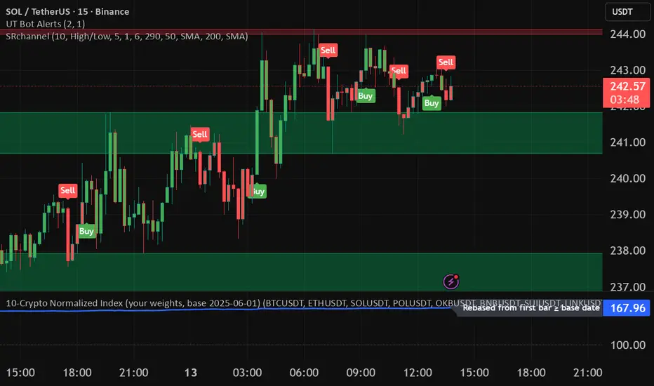
Simplified Market ForecastSimplified Market Forecast Indicator
This indicator pairs nicely with the Contrarian 100 MA and can be located here:
Overview
The "Simplified Market Forecast" (SMF) indicator is a streamlined technical analysis tool designed for traders to identify potential buy and sell opportunities based on a momentum-based oscillator. By analyzing price movements relative to a defined lookback period, SMF generates clear buy and sell signals when the oscillator crosses customizable threshold levels. This indicator is versatile, suitable for various markets (e.g., forex, stocks, cryptocurrencies), and optimized for daily timeframes, though it can be adapted to other timeframes with proper testing. Its intuitive design and visual cues make it accessible for both novice and experienced traders.
How It Works
The SMF indicator calculates a momentum oscillator based on the price’s position within a specified range over a user-defined lookback period. It then smooths this value to reduce noise and plots the result as a line in a separate lower pane. Buy and sell signals are generated when the smoothed oscillator crosses above a user-defined buy level or below a user-defined sell level, respectively. These signals are visualized as triangles either on the main chart or in the lower pane, with a table displaying the current ticker and oscillator value for quick reference.
Key Components
Momentum Oscillator: The indicator measures the price’s position relative to the highest high and lowest low over a specified period, normalized to a 0–100 scale.
Signal Generation: Buy signals occur when the oscillator crosses above the buy level (default: 15), indicating potential oversold conditions. Sell signals occur when the oscillator crosses below the sell level (default: 85), suggesting potential overbought conditions.
Visual Aids: The indicator includes customizable horizontal lines for buy and sell levels, shaded zones for clarity, and a table showing the ticker and current oscillator value.
Mathematical Concepts
Oscillator Calculation: The indicator uses the following formula to compute the raw oscillator value:
c1I = close - lowest(low, medLen)
c2I = highest(high, medLen) - lowest(low, medLen)
fastK_I = (c1I / c2I) * 100
The result is smoothed using a 5-period Simple Moving Average (SMA) to produce the final oscillator value (inter).
Signal Logic:
A buy signal is triggered when the smoothed oscillator crosses above the buy level (ta.crossover(inter, buyLevel)).
A sell signal is triggered when the smoothed oscillator crosses below the sell level (ta.crossunder(inter, sellLevel)).
Entry and Exit Rules
Buy Signal (Blue Triangle): Triggered when the oscillator crosses above the buy level (default: 15), indicating a potential oversold condition and a buying opportunity. The signal appears as a blue triangle either below the price bar (if plotted on the main chart) or at the bottom of the lower pane.
Sell Signal (White Triangle): Triggered when the oscillator crosses below the sell level (default: 85), indicating a potential overbought condition and a selling opportunity. The signal appears as a white triangle either above the price bar (if plotted on the main chart) or at the top of the lower pane.
Exit Rules: Traders can exit positions when an opposite signal occurs (e.g., exit a buy on a sell signal) or based on additional technical analysis tools (e.g., support/resistance, trendlines). Always apply proper risk management.
Recommended Usage
The SMF indicator is optimized for the daily timeframe but can be adapted to other timeframes (e.g., 1H, 4H) with careful testing. It performs best in markets with clear momentum shifts, such as trending or range-bound conditions. Traders should:
Backtest the indicator on their chosen asset and timeframe to validate signal reliability.
Combine with other indicators (e.g., moving averages, support/resistance) or price action for confirmation.
Adjust the lookback period and buy/sell levels to suit market volatility and trading style.
Customization Options
Intermediate Length: Adjust the lookback period for the oscillator calculation (default: 31 bars).
Buy/Sell Levels: Customize the threshold levels for buy (default: 15) and sell (default: 85) signals.
Colors: Modify the colors of the oscillator line, buy/sell signals, and threshold lines.
Signal Display: Toggle whether signals appear on the main chart or in the lower pane.
Visual Aids: The indicator includes dotted horizontal lines at the buy (green) and sell (red) levels, with shaded zones between 0–buy level (green) and sell level–100 (red) for clarity.
Ticker Table: A table in the top-right corner displays the current ticker and oscillator value (in percentage), with customizable colors.
Why Use This Indicator?
The "Simplified Market Forecast" indicator provides a straightforward, momentum-based approach to identifying potential reversals in overbought or oversold markets. Its clear signals, customizable settings, and visual aids make it easy to integrate into various trading strategies. Whether you’re a swing trader or a day trader, SMF offers a reliable tool to enhance decision-making and improve market timing.
Tips for Users
Test the indicator thoroughly on your chosen asset and timeframe to optimize settings.
Use in conjunction with other technical tools for stronger trade confirmation.
Adjust the buy and sell levels based on market conditions (e.g., lower levels for less volatile markets).
Monitor the ticker table for real-time oscillator values to gauge market momentum.
Happy trading with the Simplified Market Forecast indicator!