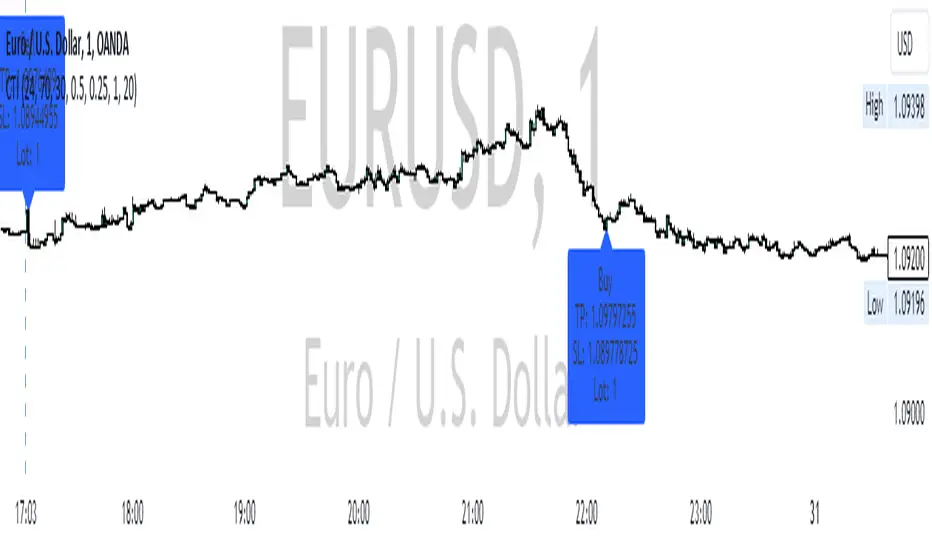
CCI RSI Trading SignalThe "CCI RSI Trading Signal" indicator combines the Commodity Channel Index (CCI) and Relative Strength Index (RSI) to provide buy and sell signals for trading. The CCI identifies potential trend reversals, while the RSI helps confirm overbought and oversold conditions.
How It Works:
The indicator generates a buy signal when the CCI crosses above -100 (indicating a potential bullish reversal) and the RSI is below the specified oversold level. On the other hand, a sell signal is produced when the CCI crosses below 100 (indicating a potential bearish reversal) and the RSI is above the specified overbought level.
Customization:
Traders can adjust the RSI and CCI periods, RSI oversold and overbought levels, as well as take profit, stop loss, and lot size settings to suit their trading preferences.
Usage:
The "CCI RSI Trading Signal" indicator can be used on various timeframes and markets to aid in decision-making, providing potential entry and exit points based on the combined analysis of CCI and RSI.
在脚本中搜索"100年黄金价格走势"
Rectified BB% for option tradingThis indicator shows the bollinger bands against the price all expressed in percentage of the mean BB value. With one sight you can see the amplitude of BB and the variation of the price, evaluate a reenter of the price in the BB.
The relative price is visualized as a candle with open/high/low/close value exspressed as percentage deviation from the BB mean
The indicator include a modified RSI, remapped from 0/100 to -100/100.
You can choose the BB parameters (length, standard deviation multiplier) and the RSI parameter (length, overbougth threshold, ovrsold threshold)
You can exclude/include the candles and the RSI line.
The indicator can be used to sell options when the volatility is high (the bollinger band is wide) and the price is reentering inside the bands.
If the price is forming a supply or demand area it can be a good opportunity to sell a bull put or a bear call
The RSI can be used as confirm of the supply/demand formation
If the bollinger band is narrow and the RSI is overbought/oversold it indicate a better opportunity to buy options
the indicator is designed to work with daily timeframe and default parameters.

imlibLibrary "imlib"
Description
The library allows you to display images in your scripts utilising the objects. You can change the image size and screen aspect ratio (the ratio of width to height which you can change if the image is too wide / tall). The library has "example()" function which you can use to see how it works. It also has a handy "logo()" function which you can use to quickly display an image by passing the "Image data string", table position, image size and aspect ratio. And of course you can use it in your own custom way by taking the "logo()" function as an example and modifying the code to your needs.
Since tables in Pinescript are limited to 100 by 100 cells, the limit for image's size is also 100x100 px. All the necessary data to display an image is passed as a string variable, and since Pinescript has a limit of 4096 characters for variables of type, that string can have a maximum length of 4096 characters, which is enough to display a 64x64px image (but can be enough to display a 100x100 image, depending on the image itself).
Below you can find the definitions of functions for this library.
_decompress(data)
: Decompresses string with data image
Parameters:
data (string)
Returns: : Array of with decompressed data
load(data)
: Splits the string with image data into components and builds an object
Parameters:
data (string)
Returns: : An object
show(imgdata, table_id, image_size, screen_ratio)
: Displays an image in a table
Parameters:
imgdata (ImgData)
table_id (table)
image_size (float)
screen_ratio (string)
Returns: : nothing
example()
: Use it as an example of how this library works and how to use it in your own scripts
Returns: : nothing
logo(imgdata, position, image_size, screen_ratio)
: Displays logo using image data string
Parameters:
imgdata (string)
position (string)
image_size (float)
screen_ratio (string)
Returns: : nothing
ImgData
Fields:
w (series__integer)
h (series__integer)
s (series__string)
pal (series__string)
data (array__string)

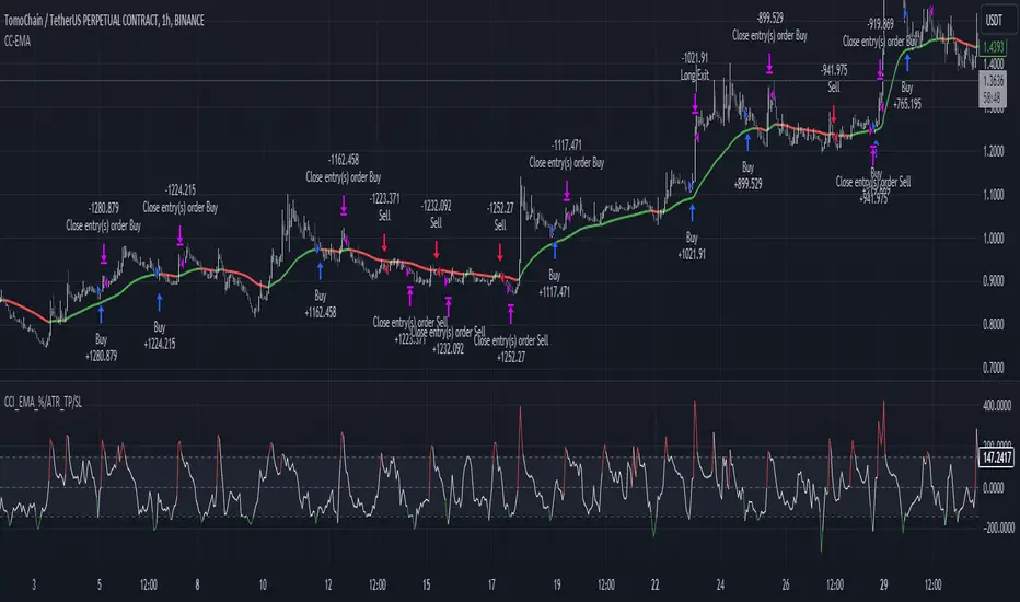
CCI+EMA Strategy with Percentage or ATR TP/SL [Alifer]This is a momentum strategy based on the Commodity Channel Index (CCI), with the aim of entering long trades in oversold conditions and short trades in overbought conditions.
Optionally, you can enable an Exponential Moving Average (EMA) to only allow trading in the direction of the larger trend. Please note that the strategy will not plot the EMA. If you want, for visual confirmation, you can add to the chart an Exponential Moving Average as a second indicator, with the same settings used in the strategy’s built-in EMA.
The strategy also allows you to set internal Stop Loss and Take Profit levels, with the option to choose between Percentage-based TP/SL or ATR-based TP/SL.
The strategy can be adapted to multiple assets and timeframes:
Pick an asset and a timeframe
Zoom back as far as possible to identify meaningful positive and negative peaks of the CCI
Set Overbought and Oversold at a rough average of the peaks you identified
Adjust TP/SL according to your risk management strategy
Like the strategy? Give it a boost!
Have any questions? Leave a comment or drop me a message.
CAUTIONARY WARNING
Please note that this is a complex trading strategy that involves several inputs and conditions. Before using it in live trading, it is highly recommended to thoroughly test it on historical data and use risk management techniques to safeguard your capital. After backtesting, it's also highly recommended to perform a first live test with a small amount. Additionally, it's essential to have a good understanding of the strategy's behavior and potential risks. Only risk what you can afford to lose .
USED INDICATORS
1 — COMMODITY CHANNEL INDEX (CCI)
The Commodity Channel Index (CCI) is a technical analysis indicator used to measure the momentum of an asset. It was developed by Donald Lambert and first published in Commodities magazine (now Futures) in 1980. Despite its name, the CCI can be used in any market and is not just for commodities. The CCI compares current price to average price over a specific time period. The indicator fluctuates above or below zero, moving into positive or negative territory. While most values, approximately 75%, fall between -100 and +100, about 25% of the values fall outside this range, indicating a lot of weakness or strength in the price movement.
The CCI was originally developed to spot long-term trend changes but has been adapted by traders for use on all markets or timeframes. Trading with multiple timeframes provides more buy or sell signals for active traders. Traders often use the CCI on the longer-term chart to establish the dominant trend and on the shorter-term chart to isolate pullbacks and generate trade signals.
CCI is calculated with the following formula:
(Typical Price - Simple Moving Average) / (0.015 x Mean Deviation)
Some trading strategies based on CCI can produce multiple false signals or losing trades when conditions turn choppy. Implementing a stop-loss strategy can help cap risk, and testing the CCI strategy for profitability on your market and timeframe is a worthy first step before initiating trades.
2 — AVERAGE TRUE RANGE (ATR)
The Average True Range (ATR) is a technical analysis indicator that measures market volatility by calculating the average range of price movements in a financial asset over a specific period of time. The ATR was developed by J. Welles Wilder Jr. and introduced in his book “New Concepts in Technical Trading Systems” in 1978.
The ATR is calculated by taking the average of the true range over a specified period. The true range is the greatest of the following:
The difference between the current high and the current low.
The difference between the previous close and the current high.
The difference between the previous close and the current low.
The ATR can be used to set stop-loss orders. One way to use ATR for stop-loss orders is to multiply the ATR by a factor (such as 2 or 3) and subtract it from the entry price for long positions or add it to the entry price for short positions. This can help traders set stop-loss orders that are more adaptive to market volatility.
3 — EXPONENTIAL MOVING AVERAGE (EMA)
The Exponential Moving Average (EMA) is a type of moving average (MA) that places a greater weight and significance on the most recent data points.
The EMA is calculated by taking the average of the true range over a specified period. The true range is the greatest of the following:
The difference between the current high and the current low.
The difference between the previous close and the current high.
The difference between the previous close and the current low.
The EMA can be used by traders to produce buy and sell signals based on crossovers and divergences from the historical average. Traders often use several different EMA lengths, such as 10-day, 50-day, and 200-day moving averages.
The formula for calculating EMA is as follows:
Compute the Simple Moving Average (SMA).
Calculate the multiplier for weighting the EMA.
Calculate the current EMA using the following formula:
EMA = Closing price x multiplier + EMA (previous day) x (1-multiplier)
STRATEGY EXPLANATION
1 — INPUTS AND PARAMETERS
The strategy uses the Commodity Channel Index (CCI) with additional options for an Exponential Moving Average (EMA), Take Profit (TP) and Stop Loss (SL).
length : The period length for the CCI calculation.
overbought : The overbought level for the CCI. When CCI crosses above this level, it may signal a potential short entry.
oversold : The oversold level for the CCI. When CCI crosses below this level, it may signal a potential long entry.
useEMA : A boolean input to enable or disable the use of Exponential Moving Average (EMA) as a filter for long and short entries.
emaLength : The period length for the EMA if it is used.
2 — CCI CALCULATION
The CCI indicator is calculated using the following formula:
(src - ma) / (0.015 * ta.dev(src, length))
src is the typical price (average of high, low, and close) and ma is the Simple Moving Average (SMA) of src over the specified length.
3 — EMA CALCULATION
If the useEMA option is enabled, an EMA is calculated with the given emaLength .
4 — TAKE PROFIT AND STOP LOSS METHODS
The strategy offers two methods for TP and SL calculations: percentage-based and ATR-based.
tpSlMethod_percentage : A boolean input to choose the percentage-based method.
tpSlMethod_atr : A boolean input to choose the ATR-based method.
5 — PERCENTAGE-BASED TP AND SL
If tpSlMethod_percentage is chosen, the strategy calculates the TP and SL levels based on a percentage of the average entry price.
tp_percentage : The percentage value for Take Profit.
sl_percentage : The percentage value for Stop Loss.
6 — ATR-BASED TP AND SL
If tpSlMethod_atr is chosen, the strategy calculates the TP and SL levels based on Average True Range (ATR).
atrLength : The period length for the ATR calculation.
atrMultiplier : A multiplier applied to the ATR to set the SL level.
riskRewardRatio : The risk-reward ratio used to calculate the TP level.
7 — ENTRY CONDITIONS
The strategy defines two conditions for entering long and short positions based on CCI and, optionally, EMA.
Long Entry: CCI crosses below the oversold level, and if useEMA is enabled, the closing price should be above the EMA.
Short Entry: CCI crosses above the overbought level, and if useEMA is enabled, the closing price should be below the EMA.
8 — TP AND SL LEVELS
The strategy calculates the TP and SL levels based on the chosen method and updates them dynamically.
For the percentage-based method, the TP and SL levels are calculated as a percentage of the average entry price.
For the ATR-based method, the TP and SL levels are calculated using the ATR value and the specified multipliers.
9 — EXIT CONDITIONS
The strategy defines exit conditions for both long and short positions.
If there is a long position, it will be closed either at TP or SL levels based on the chosen method.
If there is a short position, it will be closed either at TP or SL levels based on the chosen method.
Additionally, positions will be closed if CCI crosses back above oversold in long positions or below overbought in short positions.
10 — PLOTTING
The script plots the CCI line along with overbought and oversold levels as horizontal lines.
The CCI line is colored red when above the overbought level, green when below the oversold level, and white otherwise.
The shaded region between the overbought and oversold levels is plotted as well.
Normalized Close IndicatorThe central aspect of this indicator is the computation of a normalized close price. The normalized close price is computed by first determining the highest and lowest closing prices over a specified historical period. This highest and lowest value form the boundaries of the historical price range.
Once these bounds are established, the current closing price's position within this range is calculated. This is done by subtracting the lowest close from the current close and dividing the result by the range (the highest close minus the lowest close). This yields a value between 0 and 1, which is then multiplied by 100 to provide a percentage. This is not calculating percentile rank, but often it overlaps.
This percentage represents where the current close price stands relative to the historical price range. If the value is near 0, it indicates that the current close price is near the historical low, potentially signaling an oversold condition. Conversely, if the value is near 100, it suggests that the current close price is near the historical high, possibly indicating an overbought condition.
By using this approach, the indicator helps identify points at which the price may be considered relatively high (overbought) or low (oversold) compared to its recent historical range.
Additionally alerts are to switch from long to short and vice versa, for the most part, my strategy that incorporates this indicator is either long or short, sometimes though, the opposite bounds (high level for longs and low level for shorts) are not reached, then stop loss and take profit levels are needed.
I discovered it works fine on markets that spend most of time in a range like BTC/USD, adjustment needs to be done in user inputs and in Pine Script (length) for different exchanges, in current configuration works fine for me on Deribit Perpetuals (BTCUSD.P and ETHUSD.P), on 5 minute and 3 minute timeframes with a stop loss of 1.5% and take profit of 4.5% for BTCUSD.P and 1.7% and 5.1% for ETHUSD.P.

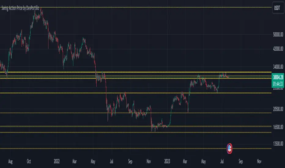
Swing Action PriceEnglish:
**Description of "Swing Action Price" TradingView Script**
"Swing Action Price" is a custom technical indicator designed to identify swing highs and swing lows in a financial market. The script calculates and plots various lines on the chart to visualize these swing points. Swing highs are points where the price has made a local peak, while swing lows are points where the price has made a local trough.
The indicator displays the following lines on the chart:
1. Dotted lines representing each individual swing high and swing low identified on different timeframes (10, 30, 60, 100, 150, 200, 700, and 1000 bars).
2. Dotted lines representing the most recent swing high and swing low for the current bar.
How the indicator works:
1. The script uses historical price data to calculate swing highs and swing lows based on specific conditions.
2. For each of the mentioned timeframes, the indicator identifies the highest high and lowest low within a defined number of bars (10, 30, 60, etc.).
3. Once a new swing high or swing low is identified, the corresponding dotted lines are drawn on the chart, extending from the previous swing point to the current one.
The "Swing Action Price" indicator can be used by traders to visually identify key support and resistance levels in the market. It helps them recognize potential trend reversals or continuation points, which may be valuable for making trading decisions.
Please note that trading indicators should always be used in conjunction with other technical and fundamental analysis tools to make informed trading choices. The "Swing Action Price" indicator is offered under the Mozilla Public License 2.0, and the developer's username is "damianjorgeportillo."
Remember that past performance is not indicative of future results, and it's essential to exercise caution and apply risk management strategies when trading financial markets.
/******************************/
Spanish:
**Descripción del Script "Swing Action Price" en TradingView**
"Swing Action Price" es un indicador técnico personalizado diseñado para identificar máximos y mínimos en un mercado financiero. El script calcula y muestra diversas líneas en el gráfico para visualizar estos puntos de inflexión. Los máximos se producen cuando el precio alcanza un pico local, mientras que los mínimos ocurren cuando el precio alcanza un valle local.
El indicador muestra las siguientes líneas en el gráfico:
1. Líneas punteadas que representan cada máximo y mínimo individual identificado en diferentes marcos de tiempo (10, 30, 60, 100, 150, 200, 700 y 1000 barras).
2. Líneas punteadas que representan el máximo y mínimo más reciente para la barra actual.
Cómo funciona el indicador:
1. El script utiliza datos históricos de precios para calcular los máximos y mínimos en función de ciertas condiciones.
2. Para cada uno de los marcos de tiempo mencionados, el indicador identifica el máximo más alto y el mínimo más bajo dentro de un número específico de barras (10, 30, 60, etc.).
3. Una vez que se identifica un nuevo máximo o mínimo, se dibujan las líneas punteadas correspondientes en el gráfico, extendiéndose desde el punto de inflexión anterior hasta el actual.
El indicador "Swing Action Price" puede ser utilizado por traders para identificar visualmente niveles clave de soporte y resistencia en el mercado. Ayuda a reconocer posibles puntos de inversión o continuación de tendencia, lo que puede ser valioso para tomar decisiones comerciales.
Por favor, ten en cuenta que los indicadores de trading siempre deben utilizarse junto con otras herramientas de análisis técnico y fundamental para tomar decisiones comerciales informadas. El indicador "Swing Action Price" se ofrece bajo la Licencia Pública de Mozilla 2.0, y el nombre de usuario del desarrollador es "damianjorgeportillo".
Recuerda que el rendimiento pasado no garantiza resultados futuros, y es esencial ser cauteloso y aplicar estrategias de gestión de riesgos al operar en los mercados financieros.
Risk to Reward - FIXED SL BacktesterDon't know how to code? No problem! TradingView is an excellent platform for you. ✅ ✅
If you have an indicator that you want to backtest using a risk-to-reward ratio or fixed take profit/stop loss levels, then the Risk to Reward - FIXED SL Backtester script is the perfect solution for you.
introducing Risk to Reward - FIXED SL Backtester Script which will allow you to test any indicator / Signal with RR or Fixed SL system
How does it work ?!
Once you connect the script to your indicator, it will analyze your entry points and perform calculations based on them. It will then open trades for you according to the specified inputs in the script settings.
HOW TO CONNECT IT to your indicator?
simply open your indicator code and add the below line of code to it
plot(Signal ? 100 : 0,"Signal",display = display.data_window)
Replace Signal with the long condition from your own indicator. You can also modify the value 100 to any number you prefer. After that, open the settings.
Once the script is connected to your indicator, you can choose from two options:
Risk To Reward Ratio System
Fixed TP/ SL System
🔸if you select the Risk to Reward System ⤵️
The Risk-to-Reward System requires the calculation of a stop loss. That's why I have included three different types of stop-loss calculations for you to choose from:
ATR Based SL
Pivot Low SL
VWAP Based SL
Your stop loss and take profit levels will be automatically calculated based on the selected stop loss method and your risk-to-reward ratio.
You can also adjust their values to match your desired risk level. The trades will be displayed on the chart.
with the ability to change their values to match your risk.
once this is done, trades will be displayed on the chart
🔸if you select the Fixed system ⤵️
You have 2 inputs, which are FIXED TP & Fixed SL
input the values you want, and trades will be on your chart...
I have also added a Breakeven feature for you.
with this Breakeven feature the trade will not just move SL to Entry ?! NO NO, it will place it above entry by a % you input yourself, so you always win! 🚀
Here is an example
Enjoy, and have fun, if you have any questions do not hesitate to ask

Enhanced WaveTrend OscillatorThe Enhanced WaveTrend Oscillator is a modified version of the original WaveTrend. The WaveTrend indicator is a popular technical analysis tool used to identify overbought and oversold conditions in the market and generate trading signals. The enhanced version addresses certain limitations of the original indicator and introduces additional features for improved analysis and comparison across assets.
WaveTrend:
The original WaveTrend indicator calculates two lines based on exponential moving averages and their relationship to the asset's price. The first line measures the distance between the asset's price and its EMA, while the second line smooths the first line over a specific period. The result is divided by 0.015 multiplied by the smoothed difference ('d' for reference). The indicator aims to identify overbought and oversold conditions by analyzing the relationship between the two lines.
In the original formula, the rudimentary estimation factor 0.015 times 'd' fails to accomodate for approximately a quarter of the data, preventing the indicator from reaching the traditional stationary levels of +-100. This limitation renders the indicator quantitatively biased, as it relies on the user's subjective adjustment of the levels. The enhanced version replaces this factor with the standard deviation of the asset's price, resulting in improved estimation accuracy and provides a more dynamic and robust outcome, we thereafter multiply the result by 100 to achieve a more traditional oscillation.
Enhancements and Features:
The enhanced version of the WaveTrend indicator addresses several limitations of the original indicator and introduces additional features-
Dynamic Estimation: The original indicator uses an arbitrary estimation factor, while the enhanced version replaces it with the standard deviation of the asset's price. This modification provides a more dynamic and accurate estimation, adapting to the specific price characteristics of each asset.
Stationary Support and Resistance Levels: The enhanced version provides stationary key support and resistance levels that range from -150 to 150. These levels are determined based on the analysis of the indicator's data and encompass more than 95% of the indicator's values. These levels offer important reference points for traders to identify potential price reversals or significant price movements.
Comparison Across Assets: The enhanced version allows for better comparison and analysis across different assets. By incorporating the standard deviation of the asset's price, the indicator provides a more consistent and comparable interpretation of the market conditions across multiple assets.
Upon closer inspection of the modification in the enhanced version, we can observe that the resulting indicator is a smoothed variation of the Z-Score!
f_ewave(src, chlen, avglen) =>
basis = ta.ema(src, chlen)
dev = ta.stdev(src, chlen)
wave = (src - basis) / dev * 100
ta.ema(wave, avglen)
Z-Score Analysis:
The Z-Score is a statistical measurement that quantifies how far a particular data point deviates from the mean in terms of standard deviations. In the enhanced version, the calculation involves determining the basis (mean) and deviation (standard deviation) of the asset's price to calculate its Z-Score, thereafter applying a smoothing technique to generate the final WaveTrend value.
Utility:
The 𝗘𝗻𝗵𝗮𝗻𝗰𝗲𝗱 𝗪𝗧 indicator offers traders and investors valuable insights into overbought and oversold conditions in the market. By analyzing the indicator's values and referencing the stationary support and resistance levels, traders can identify potential trend reversals, evaluate market strength, and make better informed analysis.
It is important to note that this indicator should be used in conjunction with other technical analysis tools and indicators to confirm trading signals and validate market dynamics.
Credit:
The 𝗘𝗻𝗵𝗮𝗻𝗰𝗲𝗱 𝗪𝗧 indicator is a modification of the original WaveTrend Oscillator developed by @LazyBear on TradingView.
Example Charts:
Discrete Fourier Transformed Money Flow IndexThe Discrete Fourier Transform Money Flow Index indicator integrates the Money Flow Index (MFI) with Discrete Fourier Transform (credit to author wbburgin - May 26 2023 ) smoothing to offer a refined and smoothed depiction of the MFI's underlying trend. The MFI is calculated using the formula: MFI = 100 - (100 / (1 + MR)), where a high MFI value indicates robust buying pressure (signaling an overbought condition), and a low MFI value indicates substantial selling pressure (signaling an oversold condition).
Why is the DFT and MFI combined?
The aim of this combination between DFT and MFI is to effectively filter out short-term fluctuations and noise, enabling a clearer assessment of the overall trend. This smoothing process enhances the reliability of the MFI by emphasizing dominant and sustained buying or selling pressures. This script executes a full DFT but only uses filtering from one frequency component. The choice to focus on the magnitude at index 0 is significant as it captures the dominant or fundamental frequency in the data. By analyzing this primary cyclic behavior, we can identify recurring patterns and potential turning points more easily. This streamlined approach simplifies interpretation and enhances efficiency by reducing complexity associated with multiple frequency components. Overall, focusing on the dominant frequency and applying it to the MFI provides a concise and actionable assessment of the underlying data.
Note: The FMFI indicator provides both smoothed and non-smoothed versions of the MFI, with the option to toggle the original non-smoothed MFI on or off in the settings.
Application
FMFI functions as a trend-following indicator. Bullish trends are denoted by the color white, while bearish trends are represented by the color purple. Circles plotted on the FMFI indicate regular bull and bear signals. Additionally, red arrows indicate a strong negative trend, while green arrows indicate a strong positive trend. These arrows are calculated based on the presence of regular bull and bear signals within overbought and oversold zones. To enhance its effectiveness, it is recommended to combine this indicator with other complementary technical analysis tools and integrate it into a comprehensive trading strategy. Traders are encouraged to explore a wide range of settings and timeframes to align the indicator with their unique trading preferences and adapt it to the current market conditions. By doing so, traders can optimize the indicator's performance and increase their potential for successful trading outcomes.
Utility
Traders and investors can employ this indicator to enhance their trend-following strategies. The white-colored components of the FMFI can help identify potential buying zones, while the purple-colored components can assist in identifying potential selling points. The red and green arrows can be used to pinpoint moments of strong bull or bear momentum, allowing traders to position themselves advantageously in their trading activities. Please note that future performance of any trading strategy is fundamentally unknowable, and past results do not guarantee future performance.

Trend Correlation HeatmapHello everyone!
I am excited to release my trend correlation heatmap, or trend heatmap for short.
Per usual, I think its important to explain the theory before we get into the use of the indicator, so let's get into the theory!
The theory:
So what is a correlation?
Correlation is the relationship one variable has to another. Correlations are the basis of everything I do as a quantitative trader. From the correlation between the same variables (i.e. autocorrelation), the correlation between other variables (i.e. VIX and SPY, SPY High and SPY Low, DXY and ES1! close, etc.) and, as well, the correlation between price and time (time series correlation).
This may sound very familiar to you, especially if you are a user, observer or follower of my ideas and/or indicators. Ninety-five percent of my indicators are a function of one of those three things. Whether it be a time series based indicator (i.e.my time series indicator), whether it be autocorrelation (my autoregressive cloud indicator or my autocorrelation oscillator) or whether it be regressive in nature (i.e. my SPY Volume weighted close, or even my expected move which uses averages in lieu of regressive approaches but is foundational in regression principles. Or even my VIX oscillator which relies on the premise of correlations between tickers.) So correlation is extremely important to me and while its true I am more of a regression trader than anything, I would argue that I am more of a correlation trader, because correlations are the backbone of how I develop math models of stocks.
What I am trying to stress here is the importance of correlations. They really truly are foundational to any type of quantitative analysis for stocks. And as such, understanding the current relationship a stock has to time is pivotal for any meaningful analysis to be conducted.
So what is correlation to time and what does it tell us?
Correlation to time, otherwise known and commonly referred to as "Time Series", is the relationship a ticker's price has to the passing of time. It is displayed in the traditional Pearson Correlation Coefficient or R value and can be any value from -1 (strong negative relationship, i.e. a strong downtrend) to + 1 (i.e. a strong positive relationship, i.e. a strong uptrend). The higher or lower the value the stronger the up or downtrend is.
As such, correlation to time tells us two very important things. These are:
a) The direction of the stock; and
b) The strength of the trend.
Let's take a look at an example:
Above we have a chart of QQQ. We can see a trendline that seems to fit well. The questions we ask as traders are:
1. What is the likelihood QQQ breaks down from this trendline?
2. What is the likelihood QQQ continues up?
3. What is the likelihood QQQ does a false breakdown?
There are numerous mathematical approaches we can take to answer these questions. For example, 1 and 2 can be answered by use of a Cumulative Distribution Density analysis (CDDA) or even a linear or loglinear regression analysis and 3 can be answered, more or less, with a linear regression analysis and standard error ascertainment, or even just a general comparison using a data science approach (such as cosine similarity or Manhattan distance).
But, the reality is, all 3 of these questions can be visualized, at least in some way, by simply looking at the correlation to time. Let's look at this chart again, this time with the correlation heatmap applied:
If we look at the indicator we can see some pivotal things. These are:
1. We have 4, very strong uptrends that span both higher AND lower timeframes. We have a strong uptrend of 0.96 on the 5 minute, 50 candle period. We have a strong uptrend at the 300 candle lookback period on the 1 minute, we have a strong uptrend on the 100 day lookback on the daily timeframe period and we have a strong uptrend on the 5 minute on the 500 candle lookback period.
2. By comparison, we have 3 downtrends, all of which have correlations less than the 4 uptrends. All of the downtrends have a correlation above -0.8 (which we would want lower than -0.8 to be very strong), and all of the uptrends are greater than + 0.80.
3. We can also see that the uptrends are not confined to the smaller timeframes. We have multiple uptrends on multiple timeframes and both short term (50 to 100 candles) and long term (up to 500 candles).
4. The overall trend is strengthening to the upside manifested by a positive Max Change and a Positive Min change (to be discussed later more in-depth).
With this, we can see that QQQ is actually very strong and likely will continue at least some upside. If we let this play out:
We continued up, had one test and then bounced.
Now, I want to specify, this indicator is not a panacea for all trading. And in relation to the 3 questions posed, they are best answered, at least quantitatively, not only by correlation but also by the aforementioned methods (CDDA, etc.) but correlation will help you get a feel for the strength or weakness present with a stock.
What are some tangible applications of the indicator?
For me, this indicator is used in many ways. Let me outline some ways I generally apply this indicator in my day and swing trading:
1. Gauging the strength of the stock: The indictor tells you the most prevalent behavior of the stock. Are there more downtrends than uptrends present? Are the downtrends present on the larger timeframes vs uptrends on the shorter indicating a possible bullish reversal? or vice versa? Are the trends strengthening or weakening? All of these things can be visualized with the indicator.
2. Setting parameters for other indicators: If you trade EMAs or SMAs, you may have a "one size fits all" approach. However, its actually better to adjust your EMA or SMA length to the actual trend itself. Take a look at this:
This is QQQ on the 1 hour with the 200 EMA with 200 standard deviation bands added. If we look at the heatmap, we can see, yes indeed 200 has a fairly strong uptrend correlation of 0.70. But the strongest hourly uptrend is actually at 400 candles, with a correlation of 0.91. So what happens if we change the EMA length and standard deviation to 400? This:
The exact areas are circled and colour coded. You can see, the 400 offers more of a better reference point of supports and resistances as well as a better overall trend fit. And this is why I never advocate for getting married to a specific EMA. If you are an EMA 200 lover or 21 or 51, know that these are not always the best depending on the trend and situation.
Components of the indicator:
Ah okay, now for the boring stuff. Let's go over the functionality of the indicator. I tried to keep it simple, so it is pretty straight forward. If we open the menu here are our options:
We have the ability to toggle whichever timeframes we want. We also have the ability to toggle on or off the legend that displays the colour codes and the Max and Min highest change.
Max and Min highest change: The max and min highest change simply display the change in correlation over the previous 14 candles. An increasing Max change means that the Max trend is strengthening. If we see an increasing Max change and an increasing Min change (the Min correlation is moving up), this means the stock is bullish. Why? Because the min (i.e. ideally a big negative number) is going up closer to the positives. Therefore, the downtrend is weakening.
If we see both the Max and Min declining (red), that means the uptrend is weakening and downtrend is strengthening. Here are some examples:
Final Thoughts:
And that is the indicator and the theory behind the indicator.
In a nutshell, to summarize, the indicator simply tracks the correlation of a ticker to time on multiple timeframes. This will allow you to make judgements about strength, sentiment and also help you adjust which tools and timeframes you are using to perform your analyses.
As well, to make the indicator more user friendly, I tried to make the colours distinctively different. I was going to do different shades but it was a little difficult to visualize. As such, I have included a toggle-able legend with a breakdown of the colour codes!
That's it my friends, I hope you find it useful!
Safe trades and leave your questions, comments and feedback below!

The Z-score The Z-score, also known as the standard score, is a statistical measurement that describes a value's relationship to the mean of a group of values. It's measured in terms of standard deviations from the mean. If a Z-score is 0, it indicates that the data point's score is identical to the mean score. Z-scores may be positive or negative, with a positive value indicating the score is above the mean and a negative score indicating it is below the mean.
The concept of Z-score was introduced by statistician Carl Friedrich Gauss as part of his "method of the least squares," which was an important step in the development of the normal distribution and Z-score tables. It's a key concept in statistics and is used in various statistical tests.
In financial analysis, Z-scores are used to determine whether a data point is usual or unusual. You can think of it as a measure of how many standard deviations an element is from the mean. For instance, a Z-score of 1.0 would denote a value that is one standard deviation from the mean. Z-scores are also used to predict probabilities, with Z-scores having a distribution that is expected to be normal.
In trading, a Z-score is used to determine how often a trading system may produce a string of winners or losers. It can help a trader to understand whether the losses or profits they see are something that the system would most likely produce, or if it's a once in a blue moon situation. This helps traders make decisions about when to start or stop a system.
I just wanted to play a bit with the Z-score I guess.
Feel free to share your findings if you discover additional applications for this strategy or identify timeframes where it appears to perform more optimally.
How it works:
This strategy is based on a statistical concept called Z-score, which measures the number of standard deviations a data point is from the mean. In other words, it helps determine how unusual or usual a data point is.
In the context of this strategy, Z-score is applied to a 10-period EMA (Exponential Moving Average) of Heikin-Ashi candlestick close prices. The Z-score is calculated over a look-back period of 25 bars.
The EMA of the Z-score is then calculated over a 20-bar period, and the upper and lower thresholds (bounds for buy and sell signals) are defined using the 90th and 10th percentiles of this EMA score.
Long positions are taken when the Z-score crosses above the lower threshold or crosses above the mid-line (50th percentile). An additional long entry is made when the Z-score crosses above the highest value the EMA has been in the past 100 periods.
Short positions are initiated when the EMA crosses below the upper threshold, lower threshold or the highest value the EMA has been in the past 100 periods.
Positions are closed when opposing entry conditions are met, for example, a long position is closed when the short entry condition is true, and vice versa.
Set your desired start date for the strategy. This can be modified in the timestamp("YYYY MM DD") function at the top of the script.

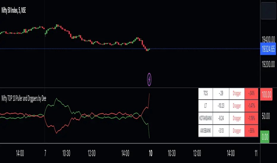
Nifty TOP 10 Puller and Drggaers by Deehi guys this is a straightforward indicator that shows the top 10 nitty pullers and dragger
How to use it ?
in the table, you can see the values of each puller and dragger well as their contribution amount and it will show if they puller or dragger
graph shows the puller and dragger using a line
both have max 100 points allocated
if they exceed the 100 points then a line will struck their ( point to remember ) it does not glitch
so it will give Ruf idea of who is strong
if buyers are strong then the green lien will always be upside
if sellers are string then the red line will always be upside
*Cross Over *
there are 2 types of cross over 1 is bull cross over other is bear cross over
when bulls are strong they will cross over the red from the bottom it showing that significantly strong
when bear is strong they will cross over the green from the bottom it shows that bear is significantly strong
hope you understand how to use it
we have limitation in trading view so we choose only 10 stock to calculate the %
ADW - Volatility MapThe ADW - Volatility Map script is a tool for traders to measure and visualize the volatility of a specific asset. It uses both the Average True Range (ATR) and True Range (TR) values in combination with the Commodity Channel Index (CCI) to provide a comprehensive map of the market's volatility.
Average True Range (ATR) : ATR is a measure of market volatility. It measures the average of true price ranges over a time period. In this script, we use it to calculate the ATR-CCI which gives us a more precise measure of volatility.
True Range (TR) : TR is the greatest distance the price moved during a period. It is used in this script to calculate the TR-CCI, adding another level of detail to our volatility measurement.
Commodity Channel Index (CCI) : CCI is a versatile indicator that can be used to identify a new trend or warn of extreme conditions. We use it to scale and compare the ATR and TR values, hence providing a relative measure of volatility.
The script interprets the CCI values and provides four different conditions for both ATR and TR:
Is Low (CCI < 0)
Is High (CCI > 0)
Is Extremely Low (CCI <= -100)
Is Extremely High (CCI >= 100)
The interpretation of these conditions is displayed on the chart using colour highlighting. When the ATR or TR are low, high, extremely low, or extremely high, the script fills the chart accordingly.
In addition, the script has an option `awaitBarConfirmation` set at the beginning. If this is true, the script will only display indicators for fully formed bars, ensuring that the indicators you see are based on confirmed information.
Note: The colours for different conditions can be customized at the beginning of the script, allowing you to personalize the visual output to match your preferences.
This script is designed to provide a visually clear and immediate understanding of the market's volatility. Use it to enhance your decision-making process and adapt your trading strategy to the current market conditions.

Monthly Gain in percentageThis scripts calculates the percentage gain in a month (previous 22 trade days).
Firstly, it calculates number of sample days
-> minimum no. of sampling duration = 22
-> maximum no. of sampling duration = increased from 22 until 0day_low > 22_day_high
Example if sampling_duration = 100
Monthly percentage gain = ((Current_Day_High_Price - 0_Day_Low_Price) * 100 / 0_Day_Low_Price) * 22 / sampling_duration

Vector3Library "Vector3"
Representation of 3D vectors and points.
This structure is used to pass 3D positions and directions around. It also contains functions for doing common vector operations.
Besides the functions listed below, other classes can be used to manipulate vectors and points as well.
For example the Quaternion and the Matrix4x4 classes are useful for rotating or transforming vectors and points.
___
**Reference:**
- github.com
- github.com
- github.com
- www.movable-type.co.uk
- docs.unity3d.com
- referencesource.microsoft.com
- github.com
\
new(x, y, z)
Create a new `Vector3`.
Parameters:
x (float) : `float` Property `x` value, (optional, default=na).
y (float) : `float` Property `y` value, (optional, default=na).
z (float) : `float` Property `z` value, (optional, default=na).
Returns: `Vector3` Generated new vector.
___
**Usage:**
```
.new(1.1, 1, 1)
```
from(value)
Create a new `Vector3` from a single value.
Parameters:
value (float) : `float` Properties positional value, (optional, default=na).
Returns: `Vector3` Generated new vector.
___
**Usage:**
```
.from(1.1)
```
from_Array(values, fill_na)
Create a new `Vector3` from a list of values, only reads up to the third item.
Parameters:
values (float ) : `array` Vector property values.
fill_na (float) : `float` Parameter value to replace missing indexes, (optional, defualt=na).
Returns: `Vector3` Generated new vector.
___
**Notes:**
- Supports any size of array, fills non available fields with `na`.
___
**Usage:**
```
.from_Array(array.from(1.1, fill_na=33))
.from_Array(array.from(1.1, 2, 3))
```
from_Vector2(values)
Create a new `Vector3` from a `Vector2`.
Parameters:
values (Vector2 type from RicardoSantos/CommonTypesMath/1) : `Vector2` Vector property values.
Returns: `Vector3` Generated new vector.
___
**Usage:**
```
.from:Vector2(.Vector2.new(1, 2.0))
```
___
**Notes:**
- Type `Vector2` from CommonTypesMath library.
from_Quaternion(values)
Create a new `Vector3` from a `Quaternion`'s `x, y, z` properties.
Parameters:
values (Quaternion type from RicardoSantos/CommonTypesMath/1) : `Quaternion` Vector property values.
Returns: `Vector3` Generated new vector.
___
**Usage:**
```
.from_Quaternion(.Quaternion.new(1, 2, 3, 4))
```
___
**Notes:**
- Type `Quaternion` from CommonTypesMath library.
from_String(expression, separator, fill_na)
Create a new `Vector3` from a list of values in a formated string.
Parameters:
expression (string) : `array` String with the list of vector properties.
separator (string) : `string` Separator between entries, (optional, default=`","`).
fill_na (float) : `float` Parameter value to replace missing indexes, (optional, defualt=na).
Returns: `Vector3` Generated new vector.
___
**Notes:**
- Supports any size of array, fills non available fields with `na`.
- `",,"` Empty fields will be ignored.
___
**Usage:**
```
.from_String("1.1", fill_na=33))
.from_String("(1.1,, 3)") // 1.1 , 3.0, NaN // empty field will be ignored!!
```
back()
Create a new `Vector3` object in the form `(0, 0, -1)`.
Returns: `Vector3` Generated new vector.
___
**Usage:**
```
.back()
```
front()
Create a new `Vector3` object in the form `(0, 0, 1)`.
Returns: `Vector3` Generated new vector.
___
**Usage:**
```
.front()
```
up()
Create a new `Vector3` object in the form `(0, 1, 0)`.
Returns: `Vector3` Generated new vector.
___
**Usage:**
```
.up()
```
down()
Create a new `Vector3` object in the form `(0, -1, 0)`.
Returns: `Vector3` Generated new vector.
___
**Usage:**
```
.down()
```
left()
Create a new `Vector3` object in the form `(-1, 0, 0)`.
Returns: `Vector3` Generated new vector.
___
**Usage:**
```
.left()
```
right()
Create a new `Vector3` object in the form `(1, 0, 0)`.
Returns: `Vector3` Generated new vector.
___
**Usage:**
```
.right()
```
zero()
Create a new `Vector3` object in the form `(0, 0, 0)`.
Returns: `Vector3` Generated new vector.
___
**Usage:**
```
.zero()
```
one()
Create a new `Vector3` object in the form `(1, 1, 1)`.
Returns: `Vector3` Generated new vector.
___
**Usage:**
```
.one()
```
minus_one()
Create a new `Vector3` object in the form `(-1, -1, -1)`.
Returns: `Vector3` Generated new vector.
___
**Usage:**
```
.minus_one()
```
unit_x()
Create a new `Vector3` object in the form `(1, 0, 0)`.
Returns: `Vector3` Generated new vector.
___
**Usage:**
```
.unit_x()
```
unit_y()
Create a new `Vector3` object in the form `(0, 1, 0)`.
Returns: `Vector3` Generated new vector.
___
**Usage:**
```
.unit_y()
```
unit_z()
Create a new `Vector3` object in the form `(0, 0, 1)`.
Returns: `Vector3` Generated new vector.
___
**Usage:**
```
.unit_z()
```
nan()
Create a new `Vector3` object in the form `(na, na, na)`.
Returns: `Vector3` Generated new vector.
___
**Usage:**
```
.nan()
```
random(max, min)
Generate a vector with random properties.
Parameters:
max (Vector3 type from RicardoSantos/CommonTypesMath/1) : `Vector3` Maximum defined range of the vector properties.
min (Vector3 type from RicardoSantos/CommonTypesMath/1) : `Vector3` Minimum defined range of the vector properties.
Returns: `Vector3` Generated new vector.
___
**Usage:**
```
.random(.from(math.pi), .from(-math.pi))
```
random(max)
Generate a vector with random properties (min set to 0.0).
Parameters:
max (Vector3 type from RicardoSantos/CommonTypesMath/1) : `Vector3` Maximum defined range of the vector properties.
Returns: `Vector3` Generated new vector.
___
**Usage:**
```
.random(.from(math.pi))
```
method copy(this)
Copy a existing `Vector3`
Namespace types: TMath.Vector3
Parameters:
this (Vector3 type from RicardoSantos/CommonTypesMath/1) : `Vector3` Source vector.
Returns: `Vector3` Generated new vector.
___
**Usage:**
```
a = .one().copy()
```
method i_add(this, other)
Modify a instance of a vector by adding a vector to it.
Namespace types: TMath.Vector3
Parameters:
this (Vector3 type from RicardoSantos/CommonTypesMath/1) : `Vector3` Source vector.
other (Vector3 type from RicardoSantos/CommonTypesMath/1) : `Vector3` Other Vector.
Returns: `Vector3` Updated source vector.
___
**Usage:**
```
a = .from(1) , a.i_add(.up())
```
method i_add(this, value)
Modify a instance of a vector by adding a vector to it.
Namespace types: TMath.Vector3
Parameters:
this (Vector3 type from RicardoSantos/CommonTypesMath/1) : `Vector3` Source vector.
value (float) : `float` Value.
Returns: `Vector3` Updated source vector.
___
**Usage:**
```
a = .from(1) , a.i_add(3.2)
```
method i_subtract(this, other)
Modify a instance of a vector by subtracting a vector to it.
Namespace types: TMath.Vector3
Parameters:
this (Vector3 type from RicardoSantos/CommonTypesMath/1) : `Vector3` Source vector.
other (Vector3 type from RicardoSantos/CommonTypesMath/1) : `Vector3` Other Vector.
Returns: `Vector3` Updated source vector.
___
**Usage:**
```
a = .from(1) , a.i_subtract(.down())
```
method i_subtract(this, value)
Modify a instance of a vector by subtracting a vector to it.
Namespace types: TMath.Vector3
Parameters:
this (Vector3 type from RicardoSantos/CommonTypesMath/1) : `Vector3` Source vector.
value (float) : `float` Value.
Returns: `Vector3` Updated source vector.
___
**Usage:**
```
a = .from(1) , a.i_subtract(3)
```
method i_multiply(this, other)
Modify a instance of a vector by multiplying a vector with it.
Namespace types: TMath.Vector3
Parameters:
this (Vector3 type from RicardoSantos/CommonTypesMath/1) : `Vector3` Source vector.
other (Vector3 type from RicardoSantos/CommonTypesMath/1) : `Vector3` Other Vector.
Returns: `Vector3` Updated source vector.
___
**Usage:**
```
a = .from(1) , a.i_multiply(.left())
```
method i_multiply(this, value)
Modify a instance of a vector by multiplying a vector with it.
Namespace types: TMath.Vector3
Parameters:
this (Vector3 type from RicardoSantos/CommonTypesMath/1) : `Vector3` Source vector.
value (float) : `float` value.
Returns: `Vector3` Updated source vector.
___
**Usage:**
```
a = .from(1) , a.i_multiply(3)
```
method i_divide(this, other)
Modify a instance of a vector by dividing it by another vector.
Namespace types: TMath.Vector3
Parameters:
this (Vector3 type from RicardoSantos/CommonTypesMath/1) : `Vector3` Source vector.
other (Vector3 type from RicardoSantos/CommonTypesMath/1) : `Vector3` Other Vector.
Returns: `Vector3` Updated source vector.
___
**Usage:**
```
a = .from(1) , a.i_divide(.forward())
```
method i_divide(this, value)
Modify a instance of a vector by dividing it by another vector.
Namespace types: TMath.Vector3
Parameters:
this (Vector3 type from RicardoSantos/CommonTypesMath/1) : `Vector3` Source vector.
value (float) : `float` Value.
Returns: `Vector3` Updated source vector.
___
**Usage:**
```
a = .from(1) , a.i_divide(3)
```
method i_mod(this, other)
Modify a instance of a vector by modulo assignment with another vector.
Namespace types: TMath.Vector3
Parameters:
this (Vector3 type from RicardoSantos/CommonTypesMath/1) : `Vector3` Source vector.
other (Vector3 type from RicardoSantos/CommonTypesMath/1) : `Vector3` Other Vector.
Returns: `Vector3` Updated source vector.
___
**Usage:**
```
a = .from(1) , a.i_mod(.back())
```
method i_mod(this, value)
Modify a instance of a vector by modulo assignment with another vector.
Namespace types: TMath.Vector3
Parameters:
this (Vector3 type from RicardoSantos/CommonTypesMath/1) : `Vector3` Source vector.
value (float) : `float` Value.
Returns: `Vector3` Updated source vector.
___
**Usage:**
```
a = .from(1) , a.i_mod(3)
```
method i_pow(this, exponent)
Modify a instance of a vector by modulo assignment with another vector.
Namespace types: TMath.Vector3
Parameters:
this (Vector3 type from RicardoSantos/CommonTypesMath/1) : `Vector3` Source vector.
exponent (Vector3 type from RicardoSantos/CommonTypesMath/1) : `Vector3` Exponent Vector.
Returns: `Vector3` Updated source vector.
___
**Usage:**
```
a = .from(1) , a.i_pow(.up())
```
method i_pow(this, exponent)
Modify a instance of a vector by modulo assignment with another vector.
Namespace types: TMath.Vector3
Parameters:
this (Vector3 type from RicardoSantos/CommonTypesMath/1) : `Vector3` Source vector.
exponent (float) : `float` Exponent Value.
Returns: `Vector3` Updated source vector.
___
**Usage:**
```
a = .from(1) , a.i_pow(2)
```
method length_squared(this)
Squared length of the vector.
Namespace types: TMath.Vector3
Parameters:
this (Vector3 type from RicardoSantos/CommonTypesMath/1)
Returns: `float` The squared length of this vector.
___
**Usage:**
```
a = .one().length_squared()
```
method magnitude_squared(this)
Squared magnitude of the vector.
Namespace types: TMath.Vector3
Parameters:
this (Vector3 type from RicardoSantos/CommonTypesMath/1) : `Vector3` Source vector.
Returns: `float` The length squared of this vector.
___
**Usage:**
```
a = .one().magnitude_squared()
```
method length(this)
Length of the vector.
Namespace types: TMath.Vector3
Parameters:
this (Vector3 type from RicardoSantos/CommonTypesMath/1) : `Vector3` Source vector.
Returns: `float` The length of this vector.
___
**Usage:**
```
a = .one().length()
```
method magnitude(this)
Magnitude of the vector.
Namespace types: TMath.Vector3
Parameters:
this (Vector3 type from RicardoSantos/CommonTypesMath/1) : `Vector3` Source vector.
Returns: `float` The Length of this vector.
___
**Usage:**
```
a = .one().magnitude()
```
method normalize(this, magnitude, eps)
Normalize a vector with a magnitude of 1(optional).
Namespace types: TMath.Vector3
Parameters:
this (Vector3 type from RicardoSantos/CommonTypesMath/1) : `Vector3` Source vector.
magnitude (float) : `float` Value to manipulate the magnitude of normalization, (optional, default=1.0).
eps (float)
Returns: `Vector3` Generated new vector.
___
**Usage:**
```
a = .new(33, 50, 100).normalize() // (x=0.283, y=0.429, z=0.858)
a = .new(33, 50, 100).normalize(2) // (x=0.142, y=0.214, z=0.429)
```
method to_String(this, precision)
Converts source vector to a string format, in the form `"(x, y, z)"`.
Namespace types: TMath.Vector3
Parameters:
this (Vector3 type from RicardoSantos/CommonTypesMath/1) : `Vector3` Source vector.
precision (string) : `string` Precision format to apply to values (optional, default='').
Returns: `string` Formated string in a `"(x, y, z)"` format.
___
**Usage:**
```
a = .one().to_String("#.###")
```
method to_Array(this)
Converts source vector to a array format.
Namespace types: TMath.Vector3
Parameters:
this (Vector3 type from RicardoSantos/CommonTypesMath/1) : `Vector3` Source vector.
Returns: `array` List of the vector properties.
___
**Usage:**
```
a = .new(1, 2, 3).to_Array()
```
method to_Vector2(this)
Converts source vector to a Vector2 in the form `x, y`.
Namespace types: TMath.Vector3
Parameters:
this (Vector3 type from RicardoSantos/CommonTypesMath/1) : `Vector3` Source vector.
Returns: `Vector2` Generated new vector.
___
**Usage:**
```
a = .from(1).to_Vector2()
```
method to_Quaternion(this, w)
Converts source vector to a Quaternion in the form `x, y, z, w`.
Namespace types: TMath.Vector3
Parameters:
this (Vector3 type from RicardoSantos/CommonTypesMath/1) : `Vector3` Sorce vector.
w (float) : `float` Property of `w` new value.
Returns: `Quaternion` Generated new vector.
___
**Usage:**
```
a = .from(1).to_Quaternion(w=1)
```
method add(this, other)
Add a vector to source vector.
Namespace types: TMath.Vector3
Parameters:
this (Vector3 type from RicardoSantos/CommonTypesMath/1) : `Vector3` Source vector.
other (Vector3 type from RicardoSantos/CommonTypesMath/1) : `Vector3` Other vector.
Returns: `Vector3` Generated new vector.
___
**Usage:**
```
a = .from(1).add(.unit_z())
```
method add(this, value)
Add a value to each property of the vector.
Namespace types: TMath.Vector3
Parameters:
this (Vector3 type from RicardoSantos/CommonTypesMath/1) : `Vector3` Source vector.
value (float) : `float` Value.
Returns: `Vector3` Generated new vector.
___
**Usage:**
```
a = .from(1).add(2.0)
```
add(value, other)
Add each property of a vector to a base value as a new vector.
Parameters:
value (float) : `float` Value.
other (Vector3 type from RicardoSantos/CommonTypesMath/1) : `Vector3` Vector.
Returns: `Vector3` Generated new vector.
___
**Usage:**
```
a = .from(2) , b = .add(1.0, a)
```
method subtract(this, other)
Subtract vector from source vector.
Namespace types: TMath.Vector3
Parameters:
this (Vector3 type from RicardoSantos/CommonTypesMath/1) : `Vector3` Source vector.
other (Vector3 type from RicardoSantos/CommonTypesMath/1) : `Vector3` Other vector.
Returns: `Vector3` Generated new vector.
___
**Usage:**
```
a = .from(1).subtract(.left())
```
method subtract(this, value)
Subtract a value from each property in source vector.
Namespace types: TMath.Vector3
Parameters:
this (Vector3 type from RicardoSantos/CommonTypesMath/1) : `Vector3` Source vector.
value (float) : `float` Value.
Returns: `Vector3` Generated new vector.
___
**Usage:**
```
a = .from(1).subtract(2.0)
```
subtract(value, other)
Subtract each property in a vector from a base value and create a new vector.
Parameters:
value (float) : `float` Value.
other (Vector3 type from RicardoSantos/CommonTypesMath/1) : `Vector3` Vector.
Returns: `Vector3` Generated new vector.
___
**Usage:**
```
a = .subtract(1.0, .right())
```
method multiply(this, other)
Multiply a vector by another.
Namespace types: TMath.Vector3
Parameters:
this (Vector3 type from RicardoSantos/CommonTypesMath/1) : `Vector3` Source vector.
other (Vector3 type from RicardoSantos/CommonTypesMath/1) : `Vector3` Other vector.
Returns: `Vector3` Generated new vector.
___
**Usage:**
```
a = .from(1).multiply(.up())
```
method multiply(this, value)
Multiply each element in source vector with a value.
Namespace types: TMath.Vector3
Parameters:
this (Vector3 type from RicardoSantos/CommonTypesMath/1) : `Vector3` Source vector.
value (float) : `float` Value.
Returns: `Vector3` Generated new vector.
___
**Usage:**
```
a = .from(1).multiply(2.0)
```
multiply(value, other)
Multiply a value with each property in a vector and create a new vector.
Parameters:
value (float) : `float` Value.
other (Vector3 type from RicardoSantos/CommonTypesMath/1) : `Vector3` Vector.
Returns: `Vector3` Generated new vector.
___
**Usage:**
```
a = .multiply(1.0, .new(1, 2, 1))
```
method divide(this, other)
Divide a vector by another.
Namespace types: TMath.Vector3
Parameters:
this (Vector3 type from RicardoSantos/CommonTypesMath/1) : `Vector3` Source vector.
other (Vector3 type from RicardoSantos/CommonTypesMath/1) : `Vector3` Other vector.
Returns: `Vector3` Generated new vector.
___
**Usage:**
```
a = .from(1).divide(.from(2))
```
method divide(this, value)
Divide each property in a vector by a value.
Namespace types: TMath.Vector3
Parameters:
this (Vector3 type from RicardoSantos/CommonTypesMath/1) : `Vector3` Source vector.
value (float) : `float` Value.
Returns: `Vector3` Generated new vector.
___
**Usage:**
```
a = .from(1).divide(2.0)
```
divide(value, other)
Divide a base value by each property in a vector and create a new vector.
Parameters:
value (float) : `float` Value.
other (Vector3 type from RicardoSantos/CommonTypesMath/1) : `Vector3` Vector.
Returns: `Vector3` Generated new vector.
___
**Usage:**
```
a = .divide(1.0, .from(2))
```
method mod(this, other)
Modulo a vector by another.
Namespace types: TMath.Vector3
Parameters:
this (Vector3 type from RicardoSantos/CommonTypesMath/1) : `Vector3` Source vector.
other (Vector3 type from RicardoSantos/CommonTypesMath/1) : `Vector3` Other vector.
Returns: `Vector3` Generated new vector.
___
**Usage:**
```
a = .from(1).mod(.from(2))
```
method mod(this, value)
Modulo each property in a vector by a value.
Namespace types: TMath.Vector3
Parameters:
this (Vector3 type from RicardoSantos/CommonTypesMath/1) : `Vector3` Source vector.
value (float) : `float` Value.
Returns: `Vector3` Generated new vector.
___
**Usage:**
```
a = .from(1).mod(2.0)
```
mod(value, other)
Modulo a base value by each property in a vector and create a new vector.
Parameters:
value (float) : `float` Value.
other (Vector3 type from RicardoSantos/CommonTypesMath/1) : `Vector3` Vector.
Returns: `Vector3` Generated new vector.
___
**Usage:**
```
a = .mod(1.0, .from(2))
```
method negate(this)
Negate a vector in the form `(zero - this)`.
Namespace types: TMath.Vector3
Parameters:
this (Vector3 type from RicardoSantos/CommonTypesMath/1) : `Vector3` Source vector.
Returns: `Vector3` Generated new vector.
___
**Usage:**
```
a = .one().negate()
```
method pow(this, other)
Modulo a vector by another.
Namespace types: TMath.Vector3
Parameters:
this (Vector3 type from RicardoSantos/CommonTypesMath/1) : `Vector3` Source vector.
other (Vector3 type from RicardoSantos/CommonTypesMath/1) : `Vector3` Other vector.
Returns: `Vector3` Generated new vector.
___
**Usage:**
```
a = .from(2).pow(.from(3))
```
method pow(this, exponent)
Raise the vector elements by a exponent.
Namespace types: TMath.Vector3
Parameters:
this (Vector3 type from RicardoSantos/CommonTypesMath/1) : `Vector3` Source vector.
exponent (float) : `float` The exponent to raise the vector by.
Returns: `Vector3` Generated new vector.
___
**Usage:**
```
a = .from(1).pow(2.0)
```
pow(value, exponent)
Raise value into a vector raised by the elements in exponent vector.
Parameters:
value (float) : `float` Base value.
exponent (Vector3 type from RicardoSantos/CommonTypesMath/1) : `Vector3` The exponent to raise the vector of base value by.
Returns: `Vector3` Generated new vector.
___
**Usage:**
```
a = .pow(1.0, .from(2))
```
method sqrt(this)
Square root of the elements in a vector.
Namespace types: TMath.Vector3
Parameters:
this (Vector3 type from RicardoSantos/CommonTypesMath/1) : `Vector3` Source vector.
Returns: `Vector3` Generated new vector.
___
**Usage:**
```
a = .from(1).sqrt()
```
method abs(this)
Absolute properties of the vector.
Namespace types: TMath.Vector3
Parameters:
this (Vector3 type from RicardoSantos/CommonTypesMath/1) : `Vector3` Source vector.
Returns: `Vector3` Generated new vector.
___
**Usage:**
```
a = .from(1).abs()
```
method max(this)
Highest property of the vector.
Namespace types: TMath.Vector3
Parameters:
this (Vector3 type from RicardoSantos/CommonTypesMath/1) : `Vector3` Source vector.
Returns: `float` Highest value amongst the vector properties.
___
**Usage:**
```
a = .new(1, 2, 3).max()
```
method min(this)
Lowest element of the vector.
Namespace types: TMath.Vector3
Parameters:
this (Vector3 type from RicardoSantos/CommonTypesMath/1) : `Vector3` Source vector.
Returns: `float` Lowest values amongst the vector properties.
___
**Usage:**
```
a = .new(1, 2, 3).min()
```
method floor(this)
Floor of vector a.
Namespace types: TMath.Vector3
Parameters:
this (Vector3 type from RicardoSantos/CommonTypesMath/1) : `Vector3` Source vector.
Returns: `Vector3` Generated new vector.
___
**Usage:**
```
a = .new(1.33, 1.66, 1.99).floor()
```
method ceil(this)
Ceil of vector a.
Namespace types: TMath.Vector3
Parameters:
this (Vector3 type from RicardoSantos/CommonTypesMath/1) : `Vector3` Source vector.
Returns: `Vector3` Generated new vector.
___
**Usage:**
```
a = .new(1.33, 1.66, 1.99).ceil()
```
method round(this)
Round of vector elements.
Namespace types: TMath.Vector3
Parameters:
this (Vector3 type from RicardoSantos/CommonTypesMath/1) : `Vector3` Source vector.
Returns: `Vector3` Generated new vector.
___
**Usage:**
```
a = .new(1.33, 1.66, 1.99).round()
```
method round(this, precision)
Round of vector elements to n digits.
Namespace types: TMath.Vector3
Parameters:
this (Vector3 type from RicardoSantos/CommonTypesMath/1) : `Vector3` Source vector.
precision (int) : `int` Number of digits to round the vector elements.
Returns: `Vector3` Generated new vector.
___
**Usage:**
```
a = .new(1.33, 1.66, 1.99).round(1) // 1.3, 1.7, 2
```
method fractional(this)
Fractional parts of vector.
Namespace types: TMath.Vector3
Parameters:
this (Vector3 type from RicardoSantos/CommonTypesMath/1) : `Vector3` Source vector.
Returns: `Vector3` Generated new vector.
___
**Usage:**
```
a = .from(1.337).fractional() // 0.337
```
method dot_product(this, other)
Dot product of two vectors.
Namespace types: TMath.Vector3
Parameters:
this (Vector3 type from RicardoSantos/CommonTypesMath/1) : `Vector3` Source vector.
other (Vector3 type from RicardoSantos/CommonTypesMath/1) : `Vector3` Other vector.
Returns: `float` Dot product.
___
**Usage:**
```
a = .from(2).dot_product(.left())
```
method cross_product(this, other)
Cross product of two vectors.
Namespace types: TMath.Vector3
Parameters:
this (Vector3 type from RicardoSantos/CommonTypesMath/1) : `Vector3` Source vector.
other (Vector3 type from RicardoSantos/CommonTypesMath/1) : `Vector3` Other vector.
Returns: `Vector3` Generated new vector.
___
**Usage:**
```
a = .from(1).cross_produc(.right())
```
method scale(this, scalar)
Scale vector by a scalar value.
Namespace types: TMath.Vector3
Parameters:
this (Vector3 type from RicardoSantos/CommonTypesMath/1) : `Vector3` Source vector.
scalar (float) : `float` Value to scale the the vector by.
Returns: `Vector3` Generated new vector.
___
**Usage:**
```
a = .from(1).scale(2)
```
method rescale(this, magnitude)
Rescale a vector to a new magnitude.
Namespace types: TMath.Vector3
Parameters:
this (Vector3 type from RicardoSantos/CommonTypesMath/1) : `Vector3` Source vector.
magnitude (float) : `float` Value to manipulate the magnitude of normalization.
Returns: `Vector3` Generated new vector.
___
**Usage:**
```
a = .from(20).rescale(1)
```
method equals(this, other)
Compares two vectors.
Namespace types: TMath.Vector3
Parameters:
this (Vector3 type from RicardoSantos/CommonTypesMath/1) : `Vector3` Source vector.
other (Vector3 type from RicardoSantos/CommonTypesMath/1) : `Vector3` Other vector.
Returns: `Vector3` Generated new vector.
___
**Usage:**
```
a = .from(1).equals(.one())
```
method sin(this)
Sine of vector.
Namespace types: TMath.Vector3
Parameters:
this (Vector3 type from RicardoSantos/CommonTypesMath/1) : `Vector3` Source vector.
Returns: `Vector3` Generated new vector.
___
**Usage:**
```
a = .from(1).sin()
```
method cos(this)
Cosine of vector.
Namespace types: TMath.Vector3
Parameters:
this (Vector3 type from RicardoSantos/CommonTypesMath/1) : `Vector3` Source vector.
Returns: `Vector3` Generated new vector.
___
**Usage:**
```
a = .from(1).cos()
```
method tan(this)
Tangent of vector.
Namespace types: TMath.Vector3
Parameters:
this (Vector3 type from RicardoSantos/CommonTypesMath/1) : `Vector3` Source vector.
Returns: `Vector3` Generated new vector.
___
**Usage:**
```
a = .from(1).tan()
```
vmax(a, b)
Highest elements of the properties from two vectors.
Parameters:
a (Vector3 type from RicardoSantos/CommonTypesMath/1) : `Vector3` Vector.
b (Vector3 type from RicardoSantos/CommonTypesMath/1) : `Vector3` Vector.
Returns: `Vector3` Generated new vector.
___
**Usage:**
```
a = .vmax(.one(), .from(2))
```
vmax(a, b, c)
Highest elements of the properties from three vectors.
Parameters:
a (Vector3 type from RicardoSantos/CommonTypesMath/1) : `Vector3` Vector.
b (Vector3 type from RicardoSantos/CommonTypesMath/1) : `Vector3` Vector.
c (Vector3 type from RicardoSantos/CommonTypesMath/1) : `Vector3` Vector.
Returns: `Vector3` Generated new vector.
___
**Usage:**
```
a = .vmax(.new(0.1, 2.5, 3.4), .from(2), .from(3))
```
vmin(a, b)
Lowest elements of the properties from two vectors.
Parameters:
a (Vector3 type from RicardoSantos/CommonTypesMath/1) : `Vector3` Vector.
b (Vector3 type from RicardoSantos/CommonTypesMath/1) : `Vector3` Vector.
Returns: `Vector3` Generated new vector.
___
**Usage:**
```
a = .vmin(.one(), .from(2))
```
vmin(a, b, c)
Lowest elements of the properties from three vectors.
Parameters:
a (Vector3 type from RicardoSantos/CommonTypesMath/1) : `Vector3` Vector.
b (Vector3 type from RicardoSantos/CommonTypesMath/1) : `Vector3` Vector.
c (Vector3 type from RicardoSantos/CommonTypesMath/1) : `Vector3` Vector.
Returns: `Vector3` Generated new vector.
___
**Usage:**
```
a = .vmin(.one(), .from(2), .new(3.3, 2.2, 0.5))
```
distance(a, b)
Distance between vector `a` and `b`.
Parameters:
a (Vector3 type from RicardoSantos/CommonTypesMath/1) : `Vector3` Source vector.
b (Vector3 type from RicardoSantos/CommonTypesMath/1) : `Vector3` Target vector.
Returns: `Vector3` Generated new vector.
___
**Usage:**
```
a = distance(.from(3), .unit_z())
```
clamp(a, min, max)
Restrict a vector between a min and max vector.
Parameters:
a (Vector3 type from RicardoSantos/CommonTypesMath/1) : `Vector3` Source vector.
min (Vector3 type from RicardoSantos/CommonTypesMath/1) : `Vector3` Minimum boundary vector.
max (Vector3 type from RicardoSantos/CommonTypesMath/1) : `Vector3` Maximum boundary vector.
Returns: `Vector3` Generated new vector.
___
**Usage:**
```
a = .clamp(a=.new(2.9, 1.5, 3.9), min=.from(2), max=.new(2.5, 3.0, 3.5))
```
clamp_magnitude(a, radius)
Vector with its magnitude clamped to a radius.
Parameters:
a (Vector3 type from RicardoSantos/CommonTypesMath/1) : `Vector3` Source vector.object, vector with properties that should be restricted to a radius.
radius (float) : `float` Maximum radius to restrict magnitude of vector.
Returns: `Vector3` Generated new vector.
___
**Usage:**
```
a = .clamp_magnitude(.from(21), 7)
```
lerp_unclamped(a, b, rate)
`Unclamped` linearly interpolates between provided vectors by a rate.
Parameters:
a (Vector3 type from RicardoSantos/CommonTypesMath/1) : `Vector3` Source vector.
b (Vector3 type from RicardoSantos/CommonTypesMath/1) : `Vector3` Target vector.
rate (float) : `float` Rate of interpolation, range(0 > 1) where 0 == source vector and 1 == target vector.
Returns: `Vector3` Generated new vector.
___
**Usage:**
```
a = .lerp_unclamped(.from(1), .from(2), 1.2)
```
lerp(a, b, rate)
Linearly interpolates between provided vectors by a rate.
Parameters:
a (Vector3 type from RicardoSantos/CommonTypesMath/1) : `Vector3` Source vector.
b (Vector3 type from RicardoSantos/CommonTypesMath/1) : `Vector3` Target vector.
rate (float) : `float` Rate of interpolation, range(0 > 1) where 0 == source vector and 1 == target vector.
Returns: `Vector3` Generated new vector.
___
**Usage:**
```
a = lerp(.one(), .from(2), 0.2)
```
herp(start, start_tangent, end, end_tangent, rate)
Hermite curve interpolation between provided vectors.
Parameters:
start (Vector3 type from RicardoSantos/CommonTypesMath/1) : `Vector3` Start vector.
start_tangent (Vector3 type from RicardoSantos/CommonTypesMath/1) : `Vector3` Start vector tangent.
end (Vector3 type from RicardoSantos/CommonTypesMath/1) : `Vector3` End vector.
end_tangent (Vector3 type from RicardoSantos/CommonTypesMath/1) : `Vector3` End vector tangent.
rate (int) : `float` Rate of the movement from `start` to `end` to get position, should be range(0 > 1).
Returns: `Vector3` Generated new vector.
___
**Usage:**
```
s = .new(0, 0, 0) , st = .new(0, 1, 1)
e = .new(1, 2, 2) , et = .new(-1, -1, 3)
h = .herp(s, st, e, et, 0.3)
```
___
**Reference:** en.m.wikibooks.org
herp_2(a, b, rate)
Hermite curve interpolation between provided vectors.
Parameters:
a (Vector3 type from RicardoSantos/CommonTypesMath/1) : `Vector3` Source vector.
b (Vector3 type from RicardoSantos/CommonTypesMath/1) : `Vector3` Target vector.
rate (Vector3 type from RicardoSantos/CommonTypesMath/1) : `Vector3` Rate of the movement per component from `start` to `end` to get position, should be range(0 > 1).
Returns: `Vector3` Generated new vector.
___
**Usage:**
```
h = .herp_2(.one(), .new(0.1, 3, 2), 0.6)
```
noise(a)
3D Noise based on Morgan McGuire @morgan3d
Parameters:
a (Vector3 type from RicardoSantos/CommonTypesMath/1) : `Vector3` Source vector.
Returns: `Vector3` Generated new vector.
___
**Usage:**
```
a = noise(.one())
```
___
**Reference:**
- thebookofshaders.com
- www.shadertoy.com
rotate(a, axis, angle)
Rotate a vector around a axis.
Parameters:
a (Vector3 type from RicardoSantos/CommonTypesMath/1) : `Vector3` Source vector.
axis (string) : `string` The plane to rotate around, `option="x", "y", "z"`.
angle (float) : `float` Angle in radians.
Returns: `Vector3` Generated new vector.
___
**Usage:**
```
a = .rotate(.from(3), 'y', math.toradians(45.0))
```
rotate_x(a, angle)
Rotate a vector on a fixed `x`.
Parameters:
a (Vector3 type from RicardoSantos/CommonTypesMath/1) : `Vector3` Source vector.
angle (float) : `float` Angle in radians.
Returns: `Vector3` Generated new vector.
___
**Usage:**
```
a = .rotate_x(.from(3), math.toradians(90.0))
```
rotate_y(a, angle)
Rotate a vector on a fixed `y`.
Parameters:
a (Vector3 type from RicardoSantos/CommonTypesMath/1) : `Vector3` Source vector.
angle (float) : `float` Angle in radians.
Returns: `Vector3` Generated new vector.
___
**Usage:**
```
a = .rotate_y(.from(3), math.toradians(90.0))
```
rotate_yaw_pitch(a, yaw, pitch)
Rotate a vector by yaw and pitch values.
Parameters:
a (Vector3 type from RicardoSantos/CommonTypesMath/1) : `Vector3` Source vector.
yaw (float) : `float` Angle in radians.
pitch (float) : `float` Angle in radians.
Returns: `Vector3` Generated new vector.
___
**Usage:**
```
a = .rotate_yaw_pitch(.from(3), math.toradians(90.0), math.toradians(45.0))
```
project(a, normal, eps)
Project a vector off a plane defined by a normal.
Parameters:
a (Vector3 type from RicardoSantos/CommonTypesMath/1) : `Vector3` Source vector.
normal (Vector3 type from RicardoSantos/CommonTypesMath/1) : `Vector3` The normal of the surface being reflected off.
eps (float) : `float` Minimum resolution to void division by zero (default=0.000001).
Returns: `Vector3` Generated new vector.
___
**Usage:**
```
a = .project(.one(), .down())
```
project_on_plane(a, normal, eps)
Projects a vector onto a plane defined by a normal orthogonal to the plane.
Parameters:
a (Vector3 type from RicardoSantos/CommonTypesMath/1) : `Vector3` Source vector.
normal (Vector3 type from RicardoSantos/CommonTypesMath/1) : `Vector3` The normal of the surface being reflected off.
eps (float) : `float` Minimum resolution to void division by zero (default=0.000001).
Returns: `Vector3` Generated new vector.
___
**Usage:**
```
a = .project_on_plane(.one(), .left())
```
project_to_2d(a, camera_position, camera_target)
Project a vector onto a two dimensions plane.
Parameters:
a (Vector3 type from RicardoSantos/CommonTypesMath/1) : `Vector3` Source vector.
camera_position (Vector3 type from RicardoSantos/CommonTypesMath/1) : `Vector3` Camera position.
camera_target (Vector3 type from RicardoSantos/CommonTypesMath/1) : `Vector3` Camera target plane position.
Returns: `Vector2` Generated new vector.
___
**Usage:**
```
a = .project_to_2d(.one(), .new(2, 2, 3), .zero())
```
reflect(a, normal)
Reflects a vector off a plane defined by a normal.
Parameters:
a (Vector3 type from RicardoSantos/CommonTypesMath/1) : `Vector3` Source vector.
normal (Vector3 type from RicardoSantos/CommonTypesMath/1) : `Vector3` The normal of the surface being reflected off.
Returns: `Vector3` Generated new vector.
___
**Usage:**
```
a = .reflect(.one(), .right())
```
angle(a, b, eps)
Angle in degrees between two vectors.
Parameters:
a (Vector3 type from RicardoSantos/CommonTypesMath/1) : `Vector3` Source vector.
b (Vector3 type from RicardoSantos/CommonTypesMath/1) : `Vector3` Target vector.
eps (float) : `float` Minimum resolution to void division by zero (default=1.0e-15).
Returns: `float` Angle value in degrees.
___
**Usage:**
```
a = .angle(.one(), .up())
```
angle_signed(a, b, axis)
Signed angle in degrees between two vectors.
Parameters:
a (Vector3 type from RicardoSantos/CommonTypesMath/1) : `Vector3` Source vector.
b (Vector3 type from RicardoSantos/CommonTypesMath/1) : `Vector3` Target vector.
axis (Vector3 type from RicardoSantos/CommonTypesMath/1) : `Vector3` Axis vector.
Returns: `float` Angle value in degrees.
___
**Usage:**
```
a = .angle_signed(.one(), .left(), .down())
```
___
**Notes:**
- The smaller of the two possible angles between the two vectors is returned, therefore the result will never
be greater than 180 degrees or smaller than -180 degrees.
- If you imagine the from and to vectors as lines on a piece of paper, both originating from the same point,
then the /axis/ vector would point up out of the paper.
- The measured angle between the two vectors would be positive in a clockwise direction and negative in an
anti-clockwise direction.
___
**Reference:**
- github.com
angle2d(a, b)
2D angle between two vectors.
Parameters:
a (Vector3 type from RicardoSantos/CommonTypesMath/1) : `Vector3` Source vector.
b (Vector3 type from RicardoSantos/CommonTypesMath/1) : `Vector3` Target vector.
Returns: `float` Angle value in degrees.
___
**Usage:**
```
a = .angle2d(.one(), .left())
```
transform_Matrix(a, M)
Transforms a vector by the given matrix.
Parameters:
a (Vector3 type from RicardoSantos/CommonTypesMath/1) : `Vector3` Source vector.
M (matrix) : `matrix` A 4x4 matrix. The transformation matrix.
Returns: `Vector3` Generated new vector.
___
**Usage:**
```
mat = matrix.new(4, 0)
mat.add_row(0, array.from(0.0, 0.0, 0.0, 1.0))
mat.add_row(1, array.from(0.0, 0.0, 1.0, 0.0))
mat.add_row(2, array.from(0.0, 1.0, 0.0, 0.0))
mat.add_row(3, array.from(1.0, 0.0, 0.0, 0.0))
b = .transform_Matrix(.one(), mat)
```
transform_M44(a, M)
Transforms a vector by the given matrix.
Parameters:
a (Vector3 type from RicardoSantos/CommonTypesMath/1) : `Vector3` Source vector.
M (M44 type from RicardoSantos/CommonTypesMath/1) : `M44` A 4x4 matrix. The transformation matrix.
Returns: `Vector3` Generated new vector.
___
**Usage:**
```
a = .transform_M44(.one(), .M44.new(0,0,0,1,0,0,1,0,0,1,0,0,1,0,0,0))
```
___
**Notes:**
- Type `M44` from `CommonTypesMath` library.
transform_normal_Matrix(a, M)
Transforms a vector by the given matrix.
Parameters:
a (Vector3 type from RicardoSantos/CommonTypesMath/1) : `Vector3` Source vector.
M (matrix) : `matrix` A 4x4 matrix. The transformation matrix.
Returns: `Vector3` Generated new vector.
___
**Usage:**
```
mat = matrix.new(4, 0)
mat.add_row(0, array.from(0.0, 0.0, 0.0, 1.0))
mat.add_row(1, array.from(0.0, 0.0, 1.0, 0.0))
mat.add_row(2, array.from(0.0, 1.0, 0.0, 0.0))
mat.add_row(3, array.from(1.0, 0.0, 0.0, 0.0))
b = .transform_normal_Matrix(.one(), mat)
```
transform_normal_M44(a, M)
Transforms a vector by the given matrix.
Parameters:
a (Vector3 type from RicardoSantos/CommonTypesMath/1) : `Vector3` Source vector.
M (M44 type from RicardoSantos/CommonTypesMath/1) : `M44` A 4x4 matrix. The transformation matrix.
Returns: `Vector3` Generated new vector.
___
**Usage:**
```
a = .transform_normal_M44(.one(), .M44.new(0,0,0,1,0,0,1,0,0,1,0,0,1,0,0,0))
```
___
**Notes:**
- Type `M44` from `CommonTypesMath` library.
transform_Array(a, rotation)
Transforms a vector by the given Quaternion rotation value.
Parameters:
a (Vector3 type from RicardoSantos/CommonTypesMath/1) : `Vector3` Source vector. The source vector to be rotated.
rotation (float ) : `array` A 4 element array. Quaternion. The rotation to apply.
Returns: `Vector3` Generated new vector.
___
**Usage:**
```
a = .transform_Array(.one(), array.from(0.2, 0.2, 0.2, 1.0))
```
___
**Reference:**
- referencesource.microsoft.com
transform_Quaternion(a, rotation)
Transforms a vector by the given Quaternion rotation value.
Parameters:
a (Vector3 type from RicardoSantos/CommonTypesMath/1) : `Vector3` Source vector. The source vector to be rotated.
rotation (Quaternion type from RicardoSantos/CommonTypesMath/1) : `array` A 4 element array. Quaternion. The rotation to apply.
Returns: `Vector3` Generated new vector.
___
**Usage:**
```
a = .transform_Quaternion(.one(), .Quaternion.new(0.2, 0.2, 0.2, 1.0))
```
___
**Notes:**
- Type `Quaternion` from `CommonTypesMath` library.
___
**Reference:**
- referencesource.microsoft.com

Non Adaptive Moving Average - Quan DaoThis Non-Adaptive Moving Average (NAMA) is my origin work. It came from the issues that I always face when using existing famous MA like EMA or RMA:
- What length should I choose for the MA for this security?
- Is there a length that works for multiple timeframes?
- Is there a length that works for multiple securities in multiple markets?
Choosing the right length for an MA is a tedious and boring work and is very subjective. One day in early 2023, I decided to create a new MA that will not be dependant a lot (non-adaptive) on the length of it, to make my life a little bit easier. The idea came from the formula of EMA and RMA:
ma = alpha * src + (1 - alpha) * ma
in which,
alpha = 1 / length for RMA
alpha = 2 / (length + 1) for EMA
I decided to use a constant alpha for the formula, which happened to be: 1.618 / 100 (i.e., golden ratio / 100)
This NAMA is using the length in the start only, after running for a while the MA value will be the same for every value of its length, which resolves good my 3 questions above.
The application of this NAMA is wide, I think.
- It can be used like a normal MA but you don't have to choose its length anymore.
- It can be used like EMA in DEMA, TEMA (I called it DNAMA, TNAMA)
- It can be used in calculating some famous indicators (RSI, TR, ...) so that these indicators will not be dependant on the length as well
In this example script, I included an EMA (in blue color) as well so that you can see how the EMA changes and NAMA stays the same when changing the value of its Length.
