ICT Killzones & MacrosICT Killzones & Macros (v1.1.5) — configurable ICT session windows + refined “macro” windows with live High/Low levels, optional extensions, next-window previews, and lightweight opening-price lines. Built to be clock-robust, timezone-aware, and performant on intraday charts.
Tip: All times are interpreted in your chosen IANA timezone (default: America/New_York) and auto-handle DST. You can rename, recolor, enable/disable, and retime every window.
What it plots
- Killzones (5) : Asia (19:00–02:00), London (02:00–05:00), NY AM (07:00–09:30), London Close (10:00–12:00), NY PM (13:30–16:00) — full-height boxes with optional header.
- Macros (8) (defaults tailored for common ICT “refined” windows): Asia-1 (18:00–21:00), Asia-2 (21:00–00:00), London-1 (01:00–04:00), AM-1 (09:45–10:15), AM-2 (10:45–11:15), Lunch (12:00–13:00), PM-1 (13:30–14:30), Power Hour (15:10–16:00).
- Live High/Low lines for the current Macro/Killzone window.
- Optional HL extension to the right until price crosses or the trading day rolls (style selectable).
- “Next” previews : earliest upcoming Macro and Killzone header; optional next-window background band.
- Opening Prices (3 lightweight time lines) : defaults 00:00, 08:30, 09:30 with right-edge labels, scoped to a session you choose (auto-cleans at session end).
- Key inputs & styling
- General : Timezone (IANA), “Sessions to show” (per window) to keep only the last N completed windows.
- Header : height (ticks), gap (ticks), fill opacity, border width/style, text size/color, toggle “Next Macro/Killzone” headers.
- Boxes : global fill opacity, global border width/style (used by both Macros & Killzones).
- High/Low : show HL, HL line style, extend on/off + extension style, optional extension labels.
- Opening Prices : enable Time 1/2/3, set HH:MM for each, session window, per-line colors, style (dotted/dashed/solid), width.
- Per-window controls : each Macro/Killzone has Enable, Session (HHMM-HHMM), Label, Fill color.
How to use (quick start)
- Set Timezone to your preference (default America/New_York).
- Toggle on the Macros and Killzones you trade. Adjust session times if needed.
- (Optional) Turn on Extend High/Low to project levels until crossed/day-roll.
- (Optional) Enable Next… headers to see the next upcoming window at a glance.
- (Optional) Configure Opening Prices (00:00 / 08:30 / 09:30 by default) and the session over which they appear.
Behavior & notes
- Time windows are computed by clock, not by guessing bar timestamps, making them robust across brokers and timeframes.
- With HL extension on, the current window’s levels extend until crossed or the end of the trading day (in your timezone). With it off, completed windows keep static HL markers (limited by “Sessions to show”).
- “Sessions to show” applies per Macro/Killzone to automatically prune older windows and keep charts snappy.
- Opening-price lines exist only within the chosen “Opening Prices Session” and are removed when it ends (keeps charts clean).
Defaults (color cues)
Killzones: Asia (blue), London (purple), NY AM (green), London Close (yellow), NY PM (orange).
Macros: neutral greys with Lunch and PM accents out of the box (all customizable).
Performance tips
- Reduce “Sessions to show” if you scroll far back in history.
- Disable “Next…” previews and/or extension labels on very slow machines.
- Narrow the “Opening Prices Session” window to exactly when you need those lines.
Changelog highlights
- v1.1.5 : Internal refinements and stability.
- v1.1.3 : Live High/Low lines for current windows + optional extension.
- v1.1.2 : Added “next Killzone” preview (to match “next Macro”).
- v1.1.0 : Defaults updated (5 KZ, 8 Macros). Removed “snap-to-killzone” behavior.
- v1.0.0 : Independent Macro vs. Killzone rendering; cleaner header logic.
- Known limitations
If your chart warns about drawings, trim “Sessions to show”.
If your broker session times differ from NY hours, adjust the sessions or change the indicator timezone.
Credits & intent
Inspired by ICT timing concepts; provided for education/mark-up, not financial advice.
Built to be flexible so you can mirror your personal playbook and journaling workflow.
在脚本中搜索"45美元兑换人民币+最新汇率"

Crypto Mean Reversion System (Pullback & Bounce)Mean Reversion Theory
The indicator operates on the principle that extreme price movements in crypto markets tend to revert toward their mean over time.
Consider this a valuable aid for your dollar-cost averaging strategy, effectively identifying periods ripe for accumulating or divesting from the market.
Research shows that:
Short-term momentum often persists briefly after surges, but extreme moves trigger mean reversion
Sharp drops exhibit strong bounce patterns, especially after capitulation events
Longer timeframes (7-day) show stronger mean reversion tendencies than shorter ones (1-day)
Timeframe Analysis
1-Day Timeframe
Pullback probabilities: 45-85% depending on surge magnitude
Bounce probabilities: 55-95% depending on drop severity
Captures immediate overextension and panic selling
More volatile but faster signal generation
7-Day Timeframe
Pullback probabilities: 50-90% (higher confidence)
Bounce probabilities: 50-90% (slightly moderated)
Filters out noise and identifies sustained trends
Stronger mean reversion signals due to extended moves
Probability Tiers
Pullback Risk (After Surges)
Moderate (45-60%): 5-10% surge → Expected -3% to -12% pullback
High (55-70%): 10-15% surge → Expected -5% to -18% pullback
Very High (65-80%): 15-25% surge → Expected -10% to -25% pullback
Extreme (75-90%): 25%+ surge → Expected -15% to -40% pullback
Bounce Probability (After Drops)
Moderate (55-65%): -5% to -10% drop → Expected +3% to +10% bounce
High (65-75%): -10% to -15% drop → Expected +6% to +18% bounce
Very High (75-85%): -15% to -25% drop → Expected +10% to +30% bounce
Extreme (85-95%): -25%+ drop → Expected +18% to +45% bounce
The probability ranges are derived from:
Crypto volatility patterns: Higher volatility than traditional assets creates stronger mean reversion
Behavioral finance: Extreme moves trigger emotional trading (FOMO/panic) that reverses
Historical backtesting: Probability estimates based on typical reversion patterns in crypto markets
Timeframe correlation: Longer timeframes show increased reversion probability due to reduced noise
Key Features
Dual-direction signals: Identifies both overbought (pullback) and oversold (bounce) conditions
Multi-timeframe confirmation: 1D and 7D analysis for different trading styles
Customizable thresholds: Adjust sensitivity based on asset volatility
Visual alerts: Color-coded labels and table for quick assessment
Risk categorization: Clear severity levels for position sizing

Dynamic Equity Allocation Model"Cash is Trash"? Not Always. Here's Why Science Beats Guesswork.
Every retail trader knows the frustration: you draw support and resistance lines, you spot patterns, you follow market gurus on social media—and still, when the next bear market hits, your portfolio bleeds red. Meanwhile, institutional investors seem to navigate market turbulence with ease, preserving capital when markets crash and participating when they rally. What's their secret?
The answer isn't insider information or access to exotic derivatives. It's systematic, scientifically validated decision-making. While most retail traders rely on subjective chart analysis and emotional reactions, professional portfolio managers use quantitative models that remove emotion from the equation and process multiple streams of market information simultaneously.
This document presents exactly such a system—not a proprietary black box available only to hedge funds, but a fully transparent, academically grounded framework that any serious investor can understand and apply. The Dynamic Equity Allocation Model (DEAM) synthesizes decades of financial research from Nobel laureates and leading academics into a practical tool for tactical asset allocation.
Stop drawing colorful lines on your chart and start thinking like a quant. This isn't about predicting where the market goes next week—it's about systematically adjusting your risk exposure based on what the data actually tells you. When valuations scream danger, when volatility spikes, when credit markets freeze, when multiple warning signals align—that's when cash isn't trash. That's when cash saves your portfolio.
The irony of "cash is trash" rhetoric is that it ignores timing. Yes, being 100% cash for decades would be disastrous. But being 100% equities through every crisis is equally foolish. The sophisticated approach is dynamic: aggressive when conditions favor risk-taking, defensive when they don't. This model shows you how to make that decision systematically, not emotionally.
Whether you're managing your own retirement portfolio or seeking to understand how institutional allocation strategies work, this comprehensive analysis provides the theoretical foundation, mathematical implementation, and practical guidance to elevate your investment approach from amateur to professional.
The choice is yours: keep hoping your chart patterns work out, or start using the same quantitative methods that professionals rely on. The tools are here. The research is cited. The methodology is explained. All you need to do is read, understand, and apply.
The Dynamic Equity Allocation Model (DEAM) is a quantitative framework for systematic allocation between equities and cash, grounded in modern portfolio theory and empirical market research. The model integrates five scientifically validated dimensions of market analysis—market regime, risk metrics, valuation, sentiment, and macroeconomic conditions—to generate dynamic allocation recommendations ranging from 0% to 100% equity exposure. This work documents the theoretical foundations, mathematical implementation, and practical application of this multi-factor approach.
1. Introduction and Theoretical Background
1.1 The Limitations of Static Portfolio Allocation
Traditional portfolio theory, as formulated by Markowitz (1952) in his seminal work "Portfolio Selection," assumes an optimal static allocation where investors distribute their wealth across asset classes according to their risk aversion. This approach rests on the assumption that returns and risks remain constant over time. However, empirical research demonstrates that this assumption does not hold in reality. Fama and French (1989) showed that expected returns vary over time and correlate with macroeconomic variables such as the spread between long-term and short-term interest rates. Campbell and Shiller (1988) demonstrated that the price-earnings ratio possesses predictive power for future stock returns, providing a foundation for dynamic allocation strategies.
The academic literature on tactical asset allocation has evolved considerably over recent decades. Ilmanen (2011) argues in "Expected Returns" that investors can improve their risk-adjusted returns by considering valuation levels, business cycles, and market sentiment. The Dynamic Equity Allocation Model presented here builds on this research tradition and operationalizes these insights into a practically applicable allocation framework.
1.2 Multi-Factor Approaches in Asset Allocation
Modern financial research has shown that different factors capture distinct aspects of market dynamics and together provide a more robust picture of market conditions than individual indicators. Ross (1976) developed the Arbitrage Pricing Theory, a model that employs multiple factors to explain security returns. Following this multi-factor philosophy, DEAM integrates five complementary analytical dimensions, each tapping different information sources and collectively enabling comprehensive market understanding.
2. Data Foundation and Data Quality
2.1 Data Sources Used
The model draws its data exclusively from publicly available market data via the TradingView platform. This transparency and accessibility is a significant advantage over proprietary models that rely on non-public data. The data foundation encompasses several categories of market information, each capturing specific aspects of market dynamics.
First, price data for the S&P 500 Index is obtained through the SPDR S&P 500 ETF (ticker: SPY). The use of a highly liquid ETF instead of the index itself has practical reasons, as ETF data is available in real-time and reflects actual tradability. In addition to closing prices, high, low, and volume data are captured, which are required for calculating advanced volatility measures.
Fundamental corporate metrics are retrieved via TradingView's Financial Data API. These include earnings per share, price-to-earnings ratio, return on equity, debt-to-equity ratio, dividend yield, and share buyback yield. Cochrane (2011) emphasizes in "Presidential Address: Discount Rates" the central importance of valuation metrics for forecasting future returns, making these fundamental data a cornerstone of the model.
Volatility indicators are represented by the CBOE Volatility Index (VIX) and related metrics. The VIX, often referred to as the market's "fear gauge," measures the implied volatility of S&P 500 index options and serves as a proxy for market participants' risk perception. Whaley (2000) describes in "The Investor Fear Gauge" the construction and interpretation of the VIX and its use as a sentiment indicator.
Macroeconomic data includes yield curve information through US Treasury bonds of various maturities and credit risk premiums through the spread between high-yield bonds and risk-free government bonds. These variables capture the macroeconomic conditions and financing conditions relevant for equity valuation. Estrella and Hardouvelis (1991) showed that the shape of the yield curve has predictive power for future economic activity, justifying the inclusion of these data.
2.2 Handling Missing Data
A practical problem when working with financial data is dealing with missing or unavailable values. The model implements a fallback system where a plausible historical average value is stored for each fundamental metric. When current data is unavailable for a specific point in time, this fallback value is used. This approach ensures that the model remains functional even during temporary data outages and avoids systematic biases from missing data. The use of average values as fallback is conservative, as it generates neither overly optimistic nor pessimistic signals.
3. Component 1: Market Regime Detection
3.1 The Concept of Market Regimes
The idea that financial markets exist in different "regimes" or states that differ in their statistical properties has a long tradition in financial science. Hamilton (1989) developed regime-switching models that allow distinguishing between different market states with different return and volatility characteristics. The practical application of this theory consists of identifying the current market state and adjusting portfolio allocation accordingly.
DEAM classifies market regimes using a scoring system that considers three main dimensions: trend strength, volatility level, and drawdown depth. This multidimensional view is more robust than focusing on individual indicators, as it captures various facets of market dynamics. Classification occurs into six distinct regimes: Strong Bull, Bull Market, Neutral, Correction, Bear Market, and Crisis.
3.2 Trend Analysis Through Moving Averages
Moving averages are among the oldest and most widely used technical indicators and have also received attention in academic literature. Brock, Lakonishok, and LeBaron (1992) examined in "Simple Technical Trading Rules and the Stochastic Properties of Stock Returns" the profitability of trading rules based on moving averages and found evidence for their predictive power, although later studies questioned the robustness of these results when considering transaction costs.
The model calculates three moving averages with different time windows: a 20-day average (approximately one trading month), a 50-day average (approximately one quarter), and a 200-day average (approximately one trading year). The relationship of the current price to these averages and the relationship of the averages to each other provide information about trend strength and direction. When the price trades above all three averages and the short-term average is above the long-term, this indicates an established uptrend. The model assigns points based on these constellations, with longer-term trends weighted more heavily as they are considered more persistent.
3.3 Volatility Regimes
Volatility, understood as the standard deviation of returns, is a central concept of financial theory and serves as the primary risk measure. However, research has shown that volatility is not constant but changes over time and occurs in clusters—a phenomenon first documented by Mandelbrot (1963) and later formalized through ARCH and GARCH models (Engle, 1982; Bollerslev, 1986).
DEAM calculates volatility not only through the classic method of return standard deviation but also uses more advanced estimators such as the Parkinson estimator and the Garman-Klass estimator. These methods utilize intraday information (high and low prices) and are more efficient than simple close-to-close volatility estimators. The Parkinson estimator (Parkinson, 1980) uses the range between high and low of a trading day and is based on the recognition that this information reveals more about true volatility than just the closing price difference. The Garman-Klass estimator (Garman and Klass, 1980) extends this approach by additionally considering opening and closing prices.
The calculated volatility is annualized by multiplying it by the square root of 252 (the average number of trading days per year), enabling standardized comparability. The model compares current volatility with the VIX, the implied volatility from option prices. A low VIX (below 15) signals market comfort and increases the regime score, while a high VIX (above 35) indicates market stress and reduces the score. This interpretation follows the empirical observation that elevated volatility is typically associated with falling markets (Schwert, 1989).
3.4 Drawdown Analysis
A drawdown refers to the percentage decline from the highest point (peak) to the lowest point (trough) during a specific period. This metric is psychologically significant for investors as it represents the maximum loss experienced. Calmar (1991) developed the Calmar Ratio, which relates return to maximum drawdown, underscoring the practical relevance of this metric.
The model calculates current drawdown as the percentage distance from the highest price of the last 252 trading days (one year). A drawdown below 3% is considered negligible and maximally increases the regime score. As drawdown increases, the score decreases progressively, with drawdowns above 20% classified as severe and indicating a crisis or bear market regime. These thresholds are empirically motivated by historical market cycles, in which corrections typically encompassed 5-10% drawdowns, bear markets 20-30%, and crises over 30%.
3.5 Regime Classification
Final regime classification occurs through aggregation of scores from trend (40% weight), volatility (30%), and drawdown (30%). The higher weighting of trend reflects the empirical observation that trend-following strategies have historically delivered robust results (Moskowitz, Ooi, and Pedersen, 2012). A total score above 80 signals a strong bull market with established uptrend, low volatility, and minimal losses. At a score below 10, a crisis situation exists requiring defensive positioning. The six regime categories enable a differentiated allocation strategy that not only distinguishes binarily between bullish and bearish but allows gradual gradations.
4. Component 2: Risk-Based Allocation
4.1 Volatility Targeting as Risk Management Approach
The concept of volatility targeting is based on the idea that investors should maximize not returns but risk-adjusted returns. Sharpe (1966, 1994) defined with the Sharpe Ratio the fundamental concept of return per unit of risk, measured as volatility. Volatility targeting goes a step further and adjusts portfolio allocation to achieve constant target volatility. This means that in times of low market volatility, equity allocation is increased, and in times of high volatility, it is reduced.
Moreira and Muir (2017) showed in "Volatility-Managed Portfolios" that strategies that adjust their exposure based on volatility forecasts achieve higher Sharpe Ratios than passive buy-and-hold strategies. DEAM implements this principle by defining a target portfolio volatility (default 12% annualized) and adjusting equity allocation to achieve it. The mathematical foundation is simple: if market volatility is 20% and target volatility is 12%, equity allocation should be 60% (12/20 = 0.6), with the remaining 40% held in cash with zero volatility.
4.2 Market Volatility Calculation
Estimating current market volatility is central to the risk-based allocation approach. The model uses several volatility estimators in parallel and selects the higher value between traditional close-to-close volatility and the Parkinson estimator. This conservative choice ensures the model does not underestimate true volatility, which could lead to excessive risk exposure.
Traditional volatility calculation uses logarithmic returns, as these have mathematically advantageous properties (additive linkage over multiple periods). The logarithmic return is calculated as ln(P_t / P_{t-1}), where P_t is the price at time t. The standard deviation of these returns over a rolling 20-trading-day window is then multiplied by √252 to obtain annualized volatility. This annualization is based on the assumption of independently identically distributed returns, which is an idealization but widely accepted in practice.
The Parkinson estimator uses additional information from the trading range (High minus Low) of each day. The formula is: σ_P = (1/√(4ln2)) × √(1/n × Σln²(H_i/L_i)) × √252, where H_i and L_i are high and low prices. Under ideal conditions, this estimator is approximately five times more efficient than the close-to-close estimator (Parkinson, 1980), as it uses more information per observation.
4.3 Drawdown-Based Position Size Adjustment
In addition to volatility targeting, the model implements drawdown-based risk control. The logic is that deep market declines often signal further losses and therefore justify exposure reduction. This behavior corresponds with the concept of path-dependent risk tolerance: investors who have already suffered losses are typically less willing to take additional risk (Kahneman and Tversky, 1979).
The model defines a maximum portfolio drawdown as a target parameter (default 15%). Since portfolio volatility and portfolio drawdown are proportional to equity allocation (assuming cash has neither volatility nor drawdown), allocation-based control is possible. For example, if the market exhibits a 25% drawdown and target portfolio drawdown is 15%, equity allocation should be at most 60% (15/25).
4.4 Dynamic Risk Adjustment
An advanced feature of DEAM is dynamic adjustment of risk-based allocation through a feedback mechanism. The model continuously estimates what actual portfolio volatility and portfolio drawdown would result at the current allocation. If risk utilization (ratio of actual to target risk) exceeds 1.0, allocation is reduced by an adjustment factor that grows exponentially with overutilization. This implements a form of dynamic feedback that avoids overexposure.
Mathematically, a risk adjustment factor r_adjust is calculated: if risk utilization u > 1, then r_adjust = exp(-0.5 × (u - 1)). This exponential function ensures that moderate overutilization is gently corrected, while strong overutilization triggers drastic reductions. The factor 0.5 in the exponent was empirically calibrated to achieve a balanced ratio between sensitivity and stability.
5. Component 3: Valuation Analysis
5.1 Theoretical Foundations of Fundamental Valuation
DEAM's valuation component is based on the fundamental premise that the intrinsic value of a security is determined by its future cash flows and that deviations between market price and intrinsic value are eventually corrected. Graham and Dodd (1934) established in "Security Analysis" the basic principles of fundamental analysis that remain relevant today. Translated into modern portfolio context, this means that markets with high valuation metrics (high price-earnings ratios) should have lower expected returns than cheaply valued markets.
Campbell and Shiller (1988) developed the Cyclically Adjusted P/E Ratio (CAPE), which smooths earnings over a full business cycle. Their empirical analysis showed that this ratio has significant predictive power for 10-year returns. Asness, Moskowitz, and Pedersen (2013) demonstrated in "Value and Momentum Everywhere" that value effects exist not only in individual stocks but also in asset classes and markets.
5.2 Equity Risk Premium as Central Valuation Metric
The Equity Risk Premium (ERP) is defined as the expected excess return of stocks over risk-free government bonds. It is the theoretical heart of valuation analysis, as it represents the compensation investors demand for bearing equity risk. Damodaran (2012) discusses in "Equity Risk Premiums: Determinants, Estimation and Implications" various methods for ERP estimation.
DEAM calculates ERP not through a single method but combines four complementary approaches with different weights. This multi-method strategy increases estimation robustness and avoids dependence on single, potentially erroneous inputs.
The first method (35% weight) uses earnings yield, calculated as 1/P/E or directly from operating earnings data, and subtracts the 10-year Treasury yield. This method follows Fed Model logic (Yardeni, 2003), although this model has theoretical weaknesses as it does not consistently treat inflation (Asness, 2003).
The second method (30% weight) extends earnings yield by share buyback yield. Share buybacks are a form of capital return to shareholders and increase value per share. Boudoukh et al. (2007) showed in "The Total Shareholder Yield" that the sum of dividend yield and buyback yield is a better predictor of future returns than dividend yield alone.
The third method (20% weight) implements the Gordon Growth Model (Gordon, 1962), which models stock value as the sum of discounted future dividends. Under constant growth g assumption: Expected Return = Dividend Yield + g. The model estimates sustainable growth as g = ROE × (1 - Payout Ratio), where ROE is return on equity and payout ratio is the ratio of dividends to earnings. This formula follows from equity theory: unretained earnings are reinvested at ROE and generate additional earnings growth.
The fourth method (15% weight) combines total shareholder yield (Dividend + Buybacks) with implied growth derived from revenue growth. This method considers that companies with strong revenue growth should generate higher future earnings, even if current valuations do not yet fully reflect this.
The final ERP is the weighted average of these four methods. A high ERP (above 4%) signals attractive valuations and increases the valuation score to 95 out of 100 possible points. A negative ERP, where stocks have lower expected returns than bonds, results in a minimal score of 10.
5.3 Quality Adjustments to Valuation
Valuation metrics alone can be misleading if not interpreted in the context of company quality. A company with a low P/E may be cheap or fundamentally problematic. The model therefore implements quality adjustments based on growth, profitability, and capital structure.
Revenue growth above 10% annually adds 10 points to the valuation score, moderate growth above 5% adds 5 points. This adjustment reflects that growth has independent value (Modigliani and Miller, 1961, extended by later growth theory). Net margin above 15% signals pricing power and operational efficiency and increases the score by 5 points, while low margins below 8% indicate competitive pressure and subtract 5 points.
Return on equity (ROE) above 20% characterizes outstanding capital efficiency and increases the score by 5 points. Piotroski (2000) showed in "Value Investing: The Use of Historical Financial Statement Information" that fundamental quality signals such as high ROE can improve the performance of value strategies.
Capital structure is evaluated through the debt-to-equity ratio. A conservative ratio below 1.0 multiplies the valuation score by 1.2, while high leverage above 2.0 applies a multiplier of 0.8. This adjustment reflects that high debt constrains financial flexibility and can become problematic in crisis times (Korteweg, 2010).
6. Component 4: Sentiment Analysis
6.1 The Role of Sentiment in Financial Markets
Investor sentiment, defined as the collective psychological attitude of market participants, influences asset prices independently of fundamental data. Baker and Wurgler (2006, 2007) developed a sentiment index and showed that periods of high sentiment are followed by overvaluations that later correct. This insight justifies integrating a sentiment component into allocation decisions.
Sentiment is difficult to measure directly but can be proxied through market indicators. The VIX is the most widely used sentiment indicator, as it aggregates implied volatility from option prices. High VIX values reflect elevated uncertainty and risk aversion, while low values signal market comfort. Whaley (2009) refers to the VIX as the "Investor Fear Gauge" and documents its role as a contrarian indicator: extremely high values typically occur at market bottoms, while low values occur at tops.
6.2 VIX-Based Sentiment Assessment
DEAM uses statistical normalization of the VIX by calculating the Z-score: z = (VIX_current - VIX_average) / VIX_standard_deviation. The Z-score indicates how many standard deviations the current VIX is from the historical average. This approach is more robust than absolute thresholds, as it adapts to the average volatility level, which can vary over longer periods.
A Z-score below -1.5 (VIX is 1.5 standard deviations below average) signals exceptionally low risk perception and adds 40 points to the sentiment score. This may seem counterintuitive—shouldn't low fear be bullish? However, the logic follows the contrarian principle: when no one is afraid, everyone is already invested, and there is limited further upside potential (Zweig, 1973). Conversely, a Z-score above 1.5 (extreme fear) adds -40 points, reflecting market panic but simultaneously suggesting potential buying opportunities.
6.3 VIX Term Structure as Sentiment Signal
The VIX term structure provides additional sentiment information. Normally, the VIX trades in contango, meaning longer-term VIX futures have higher prices than short-term. This reflects that short-term volatility is currently known, while long-term volatility is more uncertain and carries a risk premium. The model compares the VIX with VIX9D (9-day volatility) and identifies backwardation (VIX > 1.05 × VIX9D) and steep backwardation (VIX > 1.15 × VIX9D).
Backwardation occurs when short-term implied volatility is higher than longer-term, which typically happens during market stress. Investors anticipate immediate turbulence but expect calming. Psychologically, this reflects acute fear. The model subtracts 15 points for backwardation and 30 for steep backwardation, as these constellations signal elevated risk. Simon and Wiggins (2001) analyzed the VIX futures curve and showed that backwardation is associated with market declines.
6.4 Safe-Haven Flows
During crisis times, investors flee from risky assets into safe havens: gold, US dollar, and Japanese yen. This "flight to quality" is a sentiment signal. The model calculates the performance of these assets relative to stocks over the last 20 trading days. When gold or the dollar strongly rise while stocks fall, this indicates elevated risk aversion.
The safe-haven component is calculated as the difference between safe-haven performance and stock performance. Positive values (safe havens outperform) subtract up to 20 points from the sentiment score, negative values (stocks outperform) add up to 10 points. The asymmetric treatment (larger deduction for risk-off than bonus for risk-on) reflects that risk-off movements are typically sharper and more informative than risk-on phases.
Baur and Lucey (2010) examined safe-haven properties of gold and showed that gold indeed exhibits negative correlation with stocks during extreme market movements, confirming its role as crisis protection.
7. Component 5: Macroeconomic Analysis
7.1 The Yield Curve as Economic Indicator
The yield curve, represented as yields of government bonds of various maturities, contains aggregated expectations about future interest rates, inflation, and economic growth. The slope of the yield curve has remarkable predictive power for recessions. Estrella and Mishkin (1998) showed that an inverted yield curve (short-term rates higher than long-term) predicts recessions with high reliability. This is because inverted curves reflect restrictive monetary policy: the central bank raises short-term rates to combat inflation, dampening economic activity.
DEAM calculates two spread measures: the 2-year-minus-10-year spread and the 3-month-minus-10-year spread. A steep, positive curve (spreads above 1.5% and 2% respectively) signals healthy growth expectations and generates the maximum yield curve score of 40 points. A flat curve (spreads near zero) reduces the score to 20 points. An inverted curve (negative spreads) is particularly alarming and results in only 10 points.
The choice of two different spreads increases analysis robustness. The 2-10 spread is most established in academic literature, while the 3M-10Y spread is often considered more sensitive, as the 3-month rate directly reflects current monetary policy (Ang, Piazzesi, and Wei, 2006).
7.2 Credit Conditions and Spreads
Credit spreads—the yield difference between risky corporate bonds and safe government bonds—reflect risk perception in the credit market. Gilchrist and Zakrajšek (2012) constructed an "Excess Bond Premium" that measures the component of credit spreads not explained by fundamentals and showed this is a predictor of future economic activity and stock returns.
The model approximates credit spread by comparing the yield of high-yield bond ETFs (HYG) with investment-grade bond ETFs (LQD). A narrow spread below 200 basis points signals healthy credit conditions and risk appetite, contributing 30 points to the macro score. Very wide spreads above 1000 basis points (as during the 2008 financial crisis) signal credit crunch and generate zero points.
Additionally, the model evaluates whether "flight to quality" is occurring, identified through strong performance of Treasury bonds (TLT) with simultaneous weakness in high-yield bonds. This constellation indicates elevated risk aversion and reduces the credit conditions score.
7.3 Financial Stability at Corporate Level
While the yield curve and credit spreads reflect macroeconomic conditions, financial stability evaluates the health of companies themselves. The model uses the aggregated debt-to-equity ratio and return on equity of the S&P 500 as proxies for corporate health.
A low leverage level below 0.5 combined with high ROE above 15% signals robust corporate balance sheets and generates 20 points. This combination is particularly valuable as it represents both defensive strength (low debt means crisis resistance) and offensive strength (high ROE means earnings power). High leverage above 1.5 generates only 5 points, as it implies vulnerability to interest rate increases and recessions.
Korteweg (2010) showed in "The Net Benefits to Leverage" that optimal debt maximizes firm value, but excessive debt increases distress costs. At the aggregated market level, high debt indicates fragilities that can become problematic during stress phases.
8. Component 6: Crisis Detection
8.1 The Need for Systematic Crisis Detection
Financial crises are rare but extremely impactful events that suspend normal statistical relationships. During normal market volatility, diversified portfolios and traditional risk management approaches function, but during systemic crises, seemingly independent assets suddenly correlate strongly, and losses exceed historical expectations (Longin and Solnik, 2001). This justifies a separate crisis detection mechanism that operates independently of regular allocation components.
Reinhart and Rogoff (2009) documented in "This Time Is Different: Eight Centuries of Financial Folly" recurring patterns in financial crises: extreme volatility, massive drawdowns, credit market dysfunction, and asset price collapse. DEAM operationalizes these patterns into quantifiable crisis indicators.
8.2 Multi-Signal Crisis Identification
The model uses a counter-based approach where various stress signals are identified and aggregated. This methodology is more robust than relying on a single indicator, as true crises typically occur simultaneously across multiple dimensions. A single signal may be a false alarm, but the simultaneous presence of multiple signals increases confidence.
The first indicator is a VIX above the crisis threshold (default 40), adding one point. A VIX above 60 (as in 2008 and March 2020) adds two additional points, as such extreme values are historically very rare. This tiered approach captures the intensity of volatility.
The second indicator is market drawdown. A drawdown above 15% adds one point, as corrections of this magnitude can be potential harbingers of larger crises. A drawdown above 25% adds another point, as historical bear markets typically encompass 25-40% drawdowns.
The third indicator is credit market spreads above 500 basis points, adding one point. Such wide spreads occur only during significant credit market disruptions, as in 2008 during the Lehman crisis.
The fourth indicator identifies simultaneous losses in stocks and bonds. Normally, Treasury bonds act as a hedge against equity risk (negative correlation), but when both fall simultaneously, this indicates systemic liquidity problems or inflation/stagflation fears. The model checks whether both SPY and TLT have fallen more than 10% and 5% respectively over 5 trading days, adding two points.
The fifth indicator is a volume spike combined with negative returns. Extreme trading volumes (above twice the 20-day average) with falling prices signal panic selling. This adds one point.
A crisis situation is diagnosed when at least 3 indicators trigger, a severe crisis at 5 or more indicators. These thresholds were calibrated through historical backtesting to identify true crises (2008, 2020) without generating excessive false alarms.
8.3 Crisis-Based Allocation Override
When a crisis is detected, the system overrides the normal allocation recommendation and caps equity allocation at maximum 25%. In a severe crisis, the cap is set at 10%. This drastic defensive posture follows the empirical observation that crises typically require time to develop and that early reduction can avoid substantial losses (Faber, 2007).
This override logic implements a "safety first" principle: in situations of existential danger to the portfolio, capital preservation becomes the top priority. Roy (1952) formalized this approach in "Safety First and the Holding of Assets," arguing that investors should primarily minimize ruin probability.
9. Integration and Final Allocation Calculation
9.1 Component Weighting
The final allocation recommendation emerges through weighted aggregation of the five components. The standard weighting is: Market Regime 35%, Risk Management 25%, Valuation 20%, Sentiment 15%, Macro 5%. These weights reflect both theoretical considerations and empirical backtesting results.
The highest weighting of market regime is based on evidence that trend-following and momentum strategies have delivered robust results across various asset classes and time periods (Moskowitz, Ooi, and Pedersen, 2012). Current market momentum is highly informative for the near future, although it provides no information about long-term expectations.
The substantial weighting of risk management (25%) follows from the central importance of risk control. Wealth preservation is the foundation of long-term wealth creation, and systematic risk management is demonstrably value-creating (Moreira and Muir, 2017).
The valuation component receives 20% weight, based on the long-term mean reversion of valuation metrics. While valuation has limited short-term predictive power (bull and bear markets can begin at any valuation), the long-term relationship between valuation and returns is robustly documented (Campbell and Shiller, 1988).
Sentiment (15%) and Macro (5%) receive lower weights, as these factors are subtler and harder to measure. Sentiment is valuable as a contrarian indicator at extremes but less informative in normal ranges. Macro variables such as the yield curve have strong predictive power for recessions, but the transmission from recessions to stock market performance is complex and temporally variable.
9.2 Model Type Adjustments
DEAM allows users to choose between four model types: Conservative, Balanced, Aggressive, and Adaptive. This choice modifies the final allocation through additive adjustments.
Conservative mode subtracts 10 percentage points from allocation, resulting in consistently more cautious positioning. This is suitable for risk-averse investors or those with limited investment horizons. Aggressive mode adds 10 percentage points, suitable for risk-tolerant investors with long horizons.
Adaptive mode implements procyclical adjustment based on short-term momentum: if the market has risen more than 5% in the last 20 days, 5 percentage points are added; if it has declined more than 5%, 5 points are subtracted. This logic follows the observation that short-term momentum persists (Jegadeesh and Titman, 1993), but the moderate size of adjustment avoids excessive timing bets.
Balanced mode makes no adjustment and uses raw model output. This neutral setting is suitable for investors who wish to trust model recommendations unchanged.
9.3 Smoothing and Stability
The allocation resulting from aggregation undergoes final smoothing through a simple moving average over 3 periods. This smoothing is crucial for model practicality, as it reduces frequent trading and thus transaction costs. Without smoothing, the model could fluctuate between adjacent allocations with every small input change.
The choice of 3 periods as smoothing window is a compromise between responsiveness and stability. Longer smoothing would excessively delay signals and impede response to true regime changes. Shorter or no smoothing would allow too much noise. Empirical tests showed that 3-period smoothing offers an optimal ratio between these goals.
10. Visualization and Interpretation
10.1 Main Output: Equity Allocation
DEAM's primary output is a time series from 0 to 100 representing the recommended percentage allocation to equities. This representation is intuitive: 100% means full investment in stocks (specifically: an S&P 500 ETF), 0% means complete cash position, and intermediate values correspond to mixed portfolios. A value of 60% means, for example: invest 60% of wealth in SPY, hold 40% in money market instruments or cash.
The time series is color-coded to enable quick visual interpretation. Green shades represent high allocations (above 80%, bullish), red shades low allocations (below 20%, bearish), and neutral colors middle allocations. The chart background is dynamically colored based on the signal, enhancing readability in different market phases.
10.2 Dashboard Metrics
A tabular dashboard presents key metrics compactly. This includes current allocation, cash allocation (complement), an aggregated signal (BULLISH/NEUTRAL/BEARISH), current market regime, VIX level, market drawdown, and crisis status.
Additionally, fundamental metrics are displayed: P/E Ratio, Equity Risk Premium, Return on Equity, Debt-to-Equity Ratio, and Total Shareholder Yield. This transparency allows users to understand model decisions and form their own assessments.
Component scores (Regime, Risk, Valuation, Sentiment, Macro) are also displayed, each normalized on a 0-100 scale. This shows which factors primarily drive the current recommendation. If, for example, the Risk score is very low (20) while other scores are moderate (50-60), this indicates that risk management considerations are pulling allocation down.
10.3 Component Breakdown (Optional)
Advanced users can display individual components as separate lines in the chart. This enables analysis of component dynamics: do all components move synchronously, or are there divergences? Divergences can be particularly informative. If, for example, the market regime is bullish (high score) but the valuation component is very negative, this signals an overbought market not fundamentally supported—a classic "bubble warning."
This feature is disabled by default to keep the chart clean but can be activated for deeper analysis.
10.4 Confidence Bands
The model optionally displays uncertainty bands around the main allocation line. These are calculated as ±1 standard deviation of allocation over a rolling 20-period window. Wide bands indicate high volatility of model recommendations, suggesting uncertain market conditions. Narrow bands indicate stable recommendations.
This visualization implements a concept of epistemic uncertainty—uncertainty about the model estimate itself, not just market volatility. In phases where various indicators send conflicting signals, the allocation recommendation becomes more volatile, manifesting in wider bands. Users can understand this as a warning to act more cautiously or consult alternative information sources.
11. Alert System
11.1 Allocation Alerts
DEAM implements an alert system that notifies users of significant events. Allocation alerts trigger when smoothed allocation crosses certain thresholds. An alert is generated when allocation reaches 80% (from below), signaling strong bullish conditions. Another alert triggers when allocation falls to 20%, indicating defensive positioning.
These thresholds are not arbitrary but correspond with boundaries between model regimes. An allocation of 80% roughly corresponds to a clear bull market regime, while 20% corresponds to a bear market regime. Alerts at these points are therefore informative about fundamental regime shifts.
11.2 Crisis Alerts
Separate alerts trigger upon detection of crisis and severe crisis. These alerts have highest priority as they signal large risks. A crisis alert should prompt investors to review their portfolio and potentially take defensive measures beyond the automatic model recommendation (e.g., hedging through put options, rebalancing to more defensive sectors).
11.3 Regime Change Alerts
An alert triggers upon change of market regime (e.g., from Neutral to Correction, or from Bull Market to Strong Bull). Regime changes are highly informative events that typically entail substantial allocation changes. These alerts enable investors to proactively respond to changes in market dynamics.
11.4 Risk Breach Alerts
A specialized alert triggers when actual portfolio risk utilization exceeds target parameters by 20%. This is a warning signal that the risk management system is reaching its limits, possibly because market volatility is rising faster than allocation can be reduced. In such situations, investors should consider manual interventions.
12. Practical Application and Limitations
12.1 Portfolio Implementation
DEAM generates a recommendation for allocation between equities (S&P 500) and cash. Implementation by an investor can take various forms. The most direct method is using an S&P 500 ETF (e.g., SPY, VOO) for equity allocation and a money market fund or savings account for cash allocation.
A rebalancing strategy is required to synchronize actual allocation with model recommendation. Two approaches are possible: (1) rule-based rebalancing at every 10% deviation between actual and target, or (2) time-based monthly rebalancing. Both have trade-offs between responsiveness and transaction costs. Empirical evidence (Jaconetti, Kinniry, and Zilbering, 2010) suggests rebalancing frequency has moderate impact on performance, and investors should optimize based on their transaction costs.
12.2 Adaptation to Individual Preferences
The model offers numerous adjustment parameters. Component weights can be modified if investors place more or less belief in certain factors. A fundamentally-oriented investor might increase valuation weight, while a technical trader might increase regime weight.
Risk target parameters (target volatility, max drawdown) should be adapted to individual risk tolerance. Younger investors with long investment horizons can choose higher target volatility (15-18%), while retirees may prefer lower volatility (8-10%). This adjustment systematically shifts average equity allocation.
Crisis thresholds can be adjusted based on preference for sensitivity versus specificity of crisis detection. Lower thresholds (e.g., VIX > 35 instead of 40) increase sensitivity (more crises are detected) but reduce specificity (more false alarms). Higher thresholds have the reverse effect.
12.3 Limitations and Disclaimers
DEAM is based on historical relationships between indicators and market performance. There is no guarantee these relationships will persist in the future. Structural changes in markets (e.g., through regulation, technology, or central bank policy) can break established patterns. This is the fundamental problem of induction in financial science (Taleb, 2007).
The model is optimized for US equities (S&P 500). Application to other markets (international stocks, bonds, commodities) would require recalibration. The indicators and thresholds are specific to the statistical properties of the US equity market.
The model cannot eliminate losses. Even with perfect crisis prediction, an investor following the model would lose money in bear markets—just less than a buy-and-hold investor. The goal is risk-adjusted performance improvement, not risk elimination.
Transaction costs are not modeled. In practice, spreads, commissions, and taxes reduce net returns. Frequent trading can cause substantial costs. Model smoothing helps minimize this, but users should consider their specific cost situation.
The model reacts to information; it does not anticipate it. During sudden shocks (e.g., 9/11, COVID-19 lockdowns), the model can only react after price movements, not before. This limitation is inherent to all reactive systems.
12.4 Relationship to Other Strategies
DEAM is a tactical asset allocation approach and should be viewed as a complement, not replacement, for strategic asset allocation. Brinson, Hood, and Beebower (1986) showed in their influential study "Determinants of Portfolio Performance" that strategic asset allocation (long-term policy allocation) explains the majority of portfolio performance, but this leaves room for tactical adjustments based on market timing.
The model can be combined with value and momentum strategies at the individual stock level. While DEAM controls overall market exposure, within-equity decisions can be optimized through stock-picking models. This separation between strategic (market exposure) and tactical (stock selection) levels follows classical portfolio theory.
The model does not replace diversification across asset classes. A complete portfolio should also include bonds, international stocks, real estate, and alternative investments. DEAM addresses only the US equity allocation decision within a broader portfolio.
13. Scientific Foundation and Evaluation
13.1 Theoretical Consistency
DEAM's components are based on established financial theory and empirical evidence. The market regime component follows from regime-switching models (Hamilton, 1989) and trend-following literature. The risk management component implements volatility targeting (Moreira and Muir, 2017) and modern portfolio theory (Markowitz, 1952). The valuation component is based on discounted cash flow theory and empirical value research (Campbell and Shiller, 1988; Fama and French, 1992). The sentiment component integrates behavioral finance (Baker and Wurgler, 2006). The macro component uses established business cycle indicators (Estrella and Mishkin, 1998).
This theoretical grounding distinguishes DEAM from purely data-mining-based approaches that identify patterns without causal theory. Theory-guided models have greater probability of functioning out-of-sample, as they are based on fundamental mechanisms, not random correlations (Lo and MacKinlay, 1990).
13.2 Empirical Validation
While this document does not present detailed backtest analysis, it should be noted that rigorous validation of a tactical asset allocation model should include several elements:
In-sample testing establishes whether the model functions at all in the data on which it was calibrated. Out-of-sample testing is crucial: the model should be tested in time periods not used for development. Walk-forward analysis, where the model is successively trained on rolling windows and tested in the next window, approximates real implementation.
Performance metrics should be risk-adjusted. Pure return consideration is misleading, as higher returns often only compensate for higher risk. Sharpe Ratio, Sortino Ratio, Calmar Ratio, and Maximum Drawdown are relevant metrics. Comparison with benchmarks (Buy-and-Hold S&P 500, 60/40 Stock/Bond portfolio) contextualizes performance.
Robustness checks test sensitivity to parameter variation. If the model only functions at specific parameter settings, this indicates overfitting. Robust models show consistent performance over a range of plausible parameters.
13.3 Comparison with Existing Literature
DEAM fits into the broader literature on tactical asset allocation. Faber (2007) presented a simple momentum-based timing system that goes long when the market is above its 10-month average, otherwise cash. This simple system avoided large drawdowns in bear markets. DEAM can be understood as a sophistication of this approach that integrates multiple information sources.
Ilmanen (2011) discusses various timing factors in "Expected Returns" and argues for multi-factor approaches. DEAM operationalizes this philosophy. Asness, Moskowitz, and Pedersen (2013) showed that value and momentum effects work across asset classes, justifying cross-asset application of regime and valuation signals.
Ang (2014) emphasizes in "Asset Management: A Systematic Approach to Factor Investing" the importance of systematic, rule-based approaches over discretionary decisions. DEAM is fully systematic and eliminates emotional biases that plague individual investors (overconfidence, hindsight bias, loss aversion).
References
Ang, A. (2014) *Asset Management: A Systematic Approach to Factor Investing*. Oxford: Oxford University Press.
Ang, A., Piazzesi, M. and Wei, M. (2006) 'What does the yield curve tell us about GDP growth?', *Journal of Econometrics*, 131(1-2), pp. 359-403.
Asness, C.S. (2003) 'Fight the Fed Model', *The Journal of Portfolio Management*, 30(1), pp. 11-24.
Asness, C.S., Moskowitz, T.J. and Pedersen, L.H. (2013) 'Value and Momentum Everywhere', *The Journal of Finance*, 68(3), pp. 929-985.
Baker, M. and Wurgler, J. (2006) 'Investor Sentiment and the Cross-Section of Stock Returns', *The Journal of Finance*, 61(4), pp. 1645-1680.
Baker, M. and Wurgler, J. (2007) 'Investor Sentiment in the Stock Market', *Journal of Economic Perspectives*, 21(2), pp. 129-152.
Baur, D.G. and Lucey, B.M. (2010) 'Is Gold a Hedge or a Safe Haven? An Analysis of Stocks, Bonds and Gold', *Financial Review*, 45(2), pp. 217-229.
Bollerslev, T. (1986) 'Generalized Autoregressive Conditional Heteroskedasticity', *Journal of Econometrics*, 31(3), pp. 307-327.
Boudoukh, J., Michaely, R., Richardson, M. and Roberts, M.R. (2007) 'On the Importance of Measuring Payout Yield: Implications for Empirical Asset Pricing', *The Journal of Finance*, 62(2), pp. 877-915.
Brinson, G.P., Hood, L.R. and Beebower, G.L. (1986) 'Determinants of Portfolio Performance', *Financial Analysts Journal*, 42(4), pp. 39-44.
Brock, W., Lakonishok, J. and LeBaron, B. (1992) 'Simple Technical Trading Rules and the Stochastic Properties of Stock Returns', *The Journal of Finance*, 47(5), pp. 1731-1764.
Calmar, T.W. (1991) 'The Calmar Ratio', *Futures*, October issue.
Campbell, J.Y. and Shiller, R.J. (1988) 'The Dividend-Price Ratio and Expectations of Future Dividends and Discount Factors', *Review of Financial Studies*, 1(3), pp. 195-228.
Cochrane, J.H. (2011) 'Presidential Address: Discount Rates', *The Journal of Finance*, 66(4), pp. 1047-1108.
Damodaran, A. (2012) *Equity Risk Premiums: Determinants, Estimation and Implications*. Working Paper, Stern School of Business.
Engle, R.F. (1982) 'Autoregressive Conditional Heteroskedasticity with Estimates of the Variance of United Kingdom Inflation', *Econometrica*, 50(4), pp. 987-1007.
Estrella, A. and Hardouvelis, G.A. (1991) 'The Term Structure as a Predictor of Real Economic Activity', *The Journal of Finance*, 46(2), pp. 555-576.
Estrella, A. and Mishkin, F.S. (1998) 'Predicting U.S. Recessions: Financial Variables as Leading Indicators', *Review of Economics and Statistics*, 80(1), pp. 45-61.
Faber, M.T. (2007) 'A Quantitative Approach to Tactical Asset Allocation', *The Journal of Wealth Management*, 9(4), pp. 69-79.
Fama, E.F. and French, K.R. (1989) 'Business Conditions and Expected Returns on Stocks and Bonds', *Journal of Financial Economics*, 25(1), pp. 23-49.
Fama, E.F. and French, K.R. (1992) 'The Cross-Section of Expected Stock Returns', *The Journal of Finance*, 47(2), pp. 427-465.
Garman, M.B. and Klass, M.J. (1980) 'On the Estimation of Security Price Volatilities from Historical Data', *Journal of Business*, 53(1), pp. 67-78.
Gilchrist, S. and Zakrajšek, E. (2012) 'Credit Spreads and Business Cycle Fluctuations', *American Economic Review*, 102(4), pp. 1692-1720.
Gordon, M.J. (1962) *The Investment, Financing, and Valuation of the Corporation*. Homewood: Irwin.
Graham, B. and Dodd, D.L. (1934) *Security Analysis*. New York: McGraw-Hill.
Hamilton, J.D. (1989) 'A New Approach to the Economic Analysis of Nonstationary Time Series and the Business Cycle', *Econometrica*, 57(2), pp. 357-384.
Ilmanen, A. (2011) *Expected Returns: An Investor's Guide to Harvesting Market Rewards*. Chichester: Wiley.
Jaconetti, C.M., Kinniry, F.M. and Zilbering, Y. (2010) 'Best Practices for Portfolio Rebalancing', *Vanguard Research Paper*.
Jegadeesh, N. and Titman, S. (1993) 'Returns to Buying Winners and Selling Losers: Implications for Stock Market Efficiency', *The Journal of Finance*, 48(1), pp. 65-91.
Kahneman, D. and Tversky, A. (1979) 'Prospect Theory: An Analysis of Decision under Risk', *Econometrica*, 47(2), pp. 263-292.
Korteweg, A. (2010) 'The Net Benefits to Leverage', *The Journal of Finance*, 65(6), pp. 2137-2170.
Lo, A.W. and MacKinlay, A.C. (1990) 'Data-Snooping Biases in Tests of Financial Asset Pricing Models', *Review of Financial Studies*, 3(3), pp. 431-467.
Longin, F. and Solnik, B. (2001) 'Extreme Correlation of International Equity Markets', *The Journal of Finance*, 56(2), pp. 649-676.
Mandelbrot, B. (1963) 'The Variation of Certain Speculative Prices', *The Journal of Business*, 36(4), pp. 394-419.
Markowitz, H. (1952) 'Portfolio Selection', *The Journal of Finance*, 7(1), pp. 77-91.
Modigliani, F. and Miller, M.H. (1961) 'Dividend Policy, Growth, and the Valuation of Shares', *The Journal of Business*, 34(4), pp. 411-433.
Moreira, A. and Muir, T. (2017) 'Volatility-Managed Portfolios', *The Journal of Finance*, 72(4), pp. 1611-1644.
Moskowitz, T.J., Ooi, Y.H. and Pedersen, L.H. (2012) 'Time Series Momentum', *Journal of Financial Economics*, 104(2), pp. 228-250.
Parkinson, M. (1980) 'The Extreme Value Method for Estimating the Variance of the Rate of Return', *Journal of Business*, 53(1), pp. 61-65.
Piotroski, J.D. (2000) 'Value Investing: The Use of Historical Financial Statement Information to Separate Winners from Losers', *Journal of Accounting Research*, 38, pp. 1-41.
Reinhart, C.M. and Rogoff, K.S. (2009) *This Time Is Different: Eight Centuries of Financial Folly*. Princeton: Princeton University Press.
Ross, S.A. (1976) 'The Arbitrage Theory of Capital Asset Pricing', *Journal of Economic Theory*, 13(3), pp. 341-360.
Roy, A.D. (1952) 'Safety First and the Holding of Assets', *Econometrica*, 20(3), pp. 431-449.
Schwert, G.W. (1989) 'Why Does Stock Market Volatility Change Over Time?', *The Journal of Finance*, 44(5), pp. 1115-1153.
Sharpe, W.F. (1966) 'Mutual Fund Performance', *The Journal of Business*, 39(1), pp. 119-138.
Sharpe, W.F. (1994) 'The Sharpe Ratio', *The Journal of Portfolio Management*, 21(1), pp. 49-58.
Simon, D.P. and Wiggins, R.A. (2001) 'S&P Futures Returns and Contrary Sentiment Indicators', *Journal of Futures Markets*, 21(5), pp. 447-462.
Taleb, N.N. (2007) *The Black Swan: The Impact of the Highly Improbable*. New York: Random House.
Whaley, R.E. (2000) 'The Investor Fear Gauge', *The Journal of Portfolio Management*, 26(3), pp. 12-17.
Whaley, R.E. (2009) 'Understanding the VIX', *The Journal of Portfolio Management*, 35(3), pp. 98-105.
Yardeni, E. (2003) 'Stock Valuation Models', *Topical Study*, 51, Yardeni Research.
Zweig, M.E. (1973) 'An Investor Expectations Stock Price Predictive Model Using Closed-End Fund Premiums', *The Journal of Finance*, 28(1), pp. 67-78.

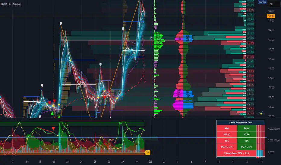
Volume Delta Volume Signals by Claudio [hapharmonic]// This Pine Script™ code is subject to the terms of the Mozilla Public License 2.0 at mozilla.org
// © hapharmonic
//@version=6
FV = format.volume
FP = format.percent
indicator('Volume Delta Volume Signals by Claudio ', format = FV, max_bars_back = 4999, max_labels_count = 500)
//------------------------------------------
// Settings |
//------------------------------------------
bool usecandle = input.bool(true, title = 'Volume on Candles',display=display.none)
color C_Up = input.color(#12cef8, title = 'Volume Buy', inline = ' ', group = 'Style')
color C_Down = input.color(#fe3f00, title = 'Volume Sell', inline = ' ', group = 'Style')
// ✅ Nueva entrada para colores de señales
color buySignalColor = input.color(color.new(color.green, 0), "Buy Signal Color", group = "Signals")
color sellSignalColor = input.color(color.new(color.red, 0), "Sell Signal Color", group = "Signals")
string P_ = input.string(position.top_right,"Position",options = ,
group = "Style",display=display.none)
string sL = input.string(size.small , 'Size Label', options = , group = 'Style',display=display.none)
string sT = input.string(size.normal, 'Size Table', options = , group = 'Style',display=display.none)
bool Label = input.bool(false, inline = 'l')
History = input.bool(true, inline = 'l')
// Inputs for EMA lengths and volume confirmation
bool MAV = input.bool(true, title = 'EMA', group = 'EMA')
string volumeOption = input.string('Use Volume Confirmation', title = 'Volume Option', options = , group = 'EMA',display=display.none)
bool useVolumeConfirmation = volumeOption == 'none' ? false : true
int emaFastLength = input(12, title = 'Fast EMA Length', group = 'EMA',display=display.none)
int emaSlowLength = input(26, title = 'Slow EMA Length', group = 'EMA',display=display.none)
int volumeConfirmationLength = input(6, title = 'Volume Confirmation Length', group = 'EMA',display=display.none)
string alert_freq = input.string(alert.freq_once_per_bar_close, title="Alert Frequency",
options= ,group = "EMA",
tooltip="If you choose once_per_bar, you will receive immediate notifications (but this may cause interference or indicator repainting).
\n However, if you choose once_per_bar_close, it will wait for the candle to confirm the signal before notifying.",display=display.none)
//------------------------------------------
// UDT_identifier |
//------------------------------------------
type OHLCV
float O = open
float H = high
float L = low
float C = close
float V = volume
type VolumeData
float buyVol
float sellVol
float pcBuy
float pcSell
bool isBuyGreater
float higherVol
float lowerVol
color higherCol
color lowerCol
//------------------------------------------
// Calculate volumes and percentages |
//------------------------------------------
calcVolumes(OHLCV ohlcv) =>
var VolumeData data = VolumeData.new()
data.buyVol := ohlcv.V * (ohlcv.C - ohlcv.L) / (ohlcv.H - ohlcv.L)
data.sellVol := ohlcv.V - data.buyVol
data.pcBuy := data.buyVol / ohlcv.V * 100
data.pcSell := 100 - data.pcBuy
data.isBuyGreater := data.buyVol > data.sellVol
data.higherVol := data.isBuyGreater ? data.buyVol : data.sellVol
data.lowerVol := data.isBuyGreater ? data.sellVol : data.buyVol
data.higherCol := data.isBuyGreater ? C_Up : C_Down
data.lowerCol := data.isBuyGreater ? C_Down : C_Up
data
//------------------------------------------
// Get volume data |
//------------------------------------------
ohlcv = OHLCV.new()
volData = calcVolumes(ohlcv)
// Plot volumes and create labels
plot(ohlcv.V, color=color.new(volData.higherCol, 90), style=plot.style_columns, title='Total',display = display.all - display.status_line)
plot(ohlcv.V, color=volData.higherCol, style=plot.style_stepline_diamond, title='Total2', linewidth = 2,display = display.pane)
plot(volData.higherVol, color=volData.higherCol, style=plot.style_columns, title='Higher Volume', display = display.all - display.status_line)
plot(volData.lowerVol , color=volData.lowerCol , style=plot.style_columns, title='Lower Volume',display = display.all - display.status_line)
S(D,F)=>str.tostring(D,F)
volStr = S(math.sign(ta.change(ohlcv.C)) * ohlcv.V, FV)
buyVolStr = S(volData.buyVol , FV )
sellVolStr = S(volData.sellVol , FV )
// ✅ MODIFICACIÓN: Porcentaje sin decimales
buyPercentStr = str.tostring(math.round(volData.pcBuy)) + " %"
sellPercentStr = str.tostring(math.round(volData.pcSell)) + " %"
totalbuyPercentC_ = volData.buyVol / (volData.buyVol + volData.sellVol) * 100
sup = not na(ohlcv.V)
if sup
TC = text.align_center
CW = color.white
var table tb = table.new(P_, 6, 6, bgcolor = na, frame_width = 2, frame_color = chart.fg_color, border_width = 1, border_color = CW)
tb.cell(0, 0, text = 'Volume Candles', text_color = #FFBF00, bgcolor = #0E2841, text_halign = TC, text_valign = TC, text_size = sT)
tb.merge_cells(0, 0, 5, 0)
tb.cell(0, 1, text = 'Current Volume', text_color = CW, bgcolor = #0B3040, text_halign = TC, text_valign = TC, text_size = sT)
tb.merge_cells(0, 1, 1, 1)
tb.cell(0, 2, text = 'Buy', text_color = #000000, bgcolor = #92D050, text_halign = TC, text_valign = TC, text_size = sT)
tb.cell(1, 2, text = 'Sell', text_color = #000000, bgcolor = #FF0000, text_halign = TC, text_valign = TC, text_size = sT)
tb.cell(0, 3, text = buyVolStr, text_color = CW, bgcolor = #074F69, text_halign = TC, text_valign = TC, text_size = sT)
tb.cell(1, 3, text = sellVolStr, text_color = CW, bgcolor = #074F69, text_halign = TC, text_valign = TC, text_size = sT)
tb.cell(0, 5, text = 'Net: ' + volStr, text_color = CW, bgcolor = #074F69, text_halign = TC, text_valign = TC, text_size = sT)
tb.merge_cells(0, 5, 1, 5)
tb.cell(0, 4, text = buyPercentStr, text_color = CW, bgcolor = #074F69, text_halign = TC, text_valign = TC, text_size = sT)
tb.cell(1, 4, text = sellPercentStr, text_color = CW, bgcolor = #074F69, text_halign = TC, text_valign = TC, text_size = sT)
cellCount = 20
filledCells = 0
for r = 5 to 1 by 1
for c = 2 to 5 by 1
if filledCells < cellCount * (totalbuyPercentC_ / 100)
tb.cell(c, r, text = '', bgcolor = C_Up)
else
tb.cell(c, r, text = '', bgcolor = C_Down)
filledCells := filledCells + 1
filledCells
if Label
sp = ' '
l = label.new(bar_index, ohlcv.V,
text=str.format('Net: {0}\nBuy: {1} ({2})\nSell: {3} ({4})\n{5}/\\\n {5}l\n {5}l',
volStr, buyVolStr, buyPercentStr, sellVolStr, sellPercentStr, sp),
style=label.style_none, textcolor=volData.higherCol, size=sL, textalign=text.align_left)
if not History
(l ).delete()
//------------------------------------------
// Draw volume levels on the candlesticks |
//------------------------------------------
float base = na,float value = na
bool uc = usecandle and sup
if volData.isBuyGreater
base := math.min(ohlcv.O, ohlcv.C)
value := base + math.abs(ohlcv.O - ohlcv.C) * (volData.pcBuy / 100)
else
base := math.max(ohlcv.O, ohlcv.C)
value := base - math.abs(ohlcv.O - ohlcv.C) * (volData.pcSell / 100)
barcolor(sup ? color.new(na, na) : ohlcv.C < ohlcv.O ? color.red : color.green,display = usecandle? display.all:display.none)
UseC = uc ? volData.higherCol:color.new(na, na)
plotcandle(uc?base:na, uc?base:na, uc?value:na, uc?value:na,
title='Body', color=UseC, bordercolor=na, wickcolor=UseC,
display = usecandle ? display.all - display.status_line : display.none, force_overlay=true,editable=false)
plotcandle(uc?ohlcv.O:na, uc?ohlcv.H:na, uc?ohlcv.L:na, uc?ohlcv.C:na,
title='Fill', color=color.new(UseC,80), bordercolor=UseC, wickcolor=UseC,
display = usecandle ? display.all - display.status_line : display.none, force_overlay=true,editable=false)
//------------------------------------------------------------
// Plot the EMA and filter out the noise with volume control. |
//------------------------------------------------------------
float emaFast = ta.ema(ohlcv.C, emaFastLength)
float emaSlow = ta.ema(ohlcv.C, emaSlowLength)
bool signal = emaFast > emaSlow
color c_signal = signal ? C_Up : C_Down
float volumeMA = ta.sma(ohlcv.V, volumeConfirmationLength)
bool crossover = ta.crossover(emaFast, emaSlow)
bool crossunder = ta.crossunder(emaFast, emaSlow)
isVolumeConfirmed(source, length, ma) =>
math.sum(source > ma ? source : 0, length) >= math.sum(source < ma ? source : 0, length)
bool ISV = isVolumeConfirmed(ohlcv.V, volumeConfirmationLength, volumeMA)
bool crossoverConfirmed = crossover and (not useVolumeConfirmation or ISV)
bool crossunderConfirmed = crossunder and (not useVolumeConfirmation or ISV)
PF = MAV ? emaFast : na
PS = MAV ? emaSlow : na
p1 = plot(PF, color = c_signal, editable = false, force_overlay = true, display = display.pane)
plot(PF, color = color.new(c_signal, 80), linewidth = 10, editable = false, force_overlay = true, display = display.pane)
plot(PF, color = color.new(c_signal, 90), linewidth = 20, editable = false, force_overlay = true, display = display.pane)
plot(PF, color = color.new(c_signal, 95), linewidth = 30, editable = false, force_overlay = true, display = display.pane)
plot(PF, color = color.new(c_signal, 98), linewidth = 45, editable = false, force_overlay = true, display = display.pane)
p2 = plot(PS, color = c_signal, editable = false, force_overlay = true, display = display.pane)
plot(PS, color = color.new(c_signal, 80), linewidth = 10, editable = false, force_overlay = true, display = display.pane)
plot(PS, color = color.new(c_signal, 90), linewidth = 20, editable = false, force_overlay = true, display = display.pane)
plot(PS, color = color.new(c_signal, 95), linewidth = 30, editable = false, force_overlay = true, display = display.pane)
plot(PS, color = color.new(c_signal, 98), linewidth = 45, editable = false, force_overlay = true, display = display.pane)
fill(p1, p2, top_value=crossover ? emaFast : emaSlow,
bottom_value =crossover ? emaSlow : emaFast,
top_color =color.new(c_signal, 80),
bottom_color =color.new(c_signal, 95)
)
// ✅ Usar colores configurables para señales
plotshape(crossoverConfirmed and MAV, style=shape.triangleup , location=location.belowbar, color=buySignalColor , size=size.small, force_overlay=true,display =display.pane)
plotshape(crossunderConfirmed and MAV, style=shape.triangledown, location=location.abovebar, color=sellSignalColor, size=size.small, force_overlay=true,display =display.pane)
string msg = '---------\n'+"Buy volume ="+buyVolStr+"\nBuy Percent = "+buyPercentStr+"\nSell volume = "+sellVolStr+"\nSell Percent = "+sellPercentStr+"\nNet = "+volStr+'\n---------'
if crossoverConfirmed
alert("Price (" + str.tostring(close) + ") Crossed over MA\n" + msg, alert_freq)
if crossunderConfirmed
alert("Price (" + str.tostring(close) + ") Crossed under MA\n" + msg, alert_freq)
RSI Z-score | Lemniscuss🧠 Introducing RSI Z-Score (RSI-Z) by Lemniscuss
🛠️ Overview
RSI Z-Score (RSI-Z) is a momentum-based market condition detector that transforms the classic Relative Strength Index (RSI) into a standardized volatility framework.
By applying Z-Score normalization to the RSI, this tool allows traders to identify statistically significant deviations in momentum — cutting through noise and highlighting high-probability turning points.
RSI-Z is optimized for trend inflection detection and overextension spotting, providing both visual clarity and actionable trade signals with dynamic labeling and optional bar coloring.
🔍 How It Works
1️⃣ RSI Foundation
The system starts with a standard RSI calculation on a user-defined source and length (default: 45).
2️⃣ Z-Score Normalization
The RSI values are standardized by subtracting their mean and dividing by the standard deviation over the same lookback.
This converts RSI into a statistical measure — revealing how many standard deviations current momentum is from its mean.
3️⃣ Threshold Logic
Two customizable thresholds define actionable zones:
• Long Threshold → Signals bullish momentum shifts when crossed upward
• Short Threshold → Signals bearish momentum shifts when crossed downward
4️⃣ Signal State Tracking
A state variable locks in a bias (Long / Short / Neutral) until an opposing trigger appears, ensuring clear and consistent market bias mapping.
✨ Key Features
🔹 Statistically Driven Momentum Detection — Moves beyond fixed RSI overbought/oversold levels by using standard deviations for adaptive accuracy.
🔹 Customizable Thresholds — Fine-tune long/short triggers for different volatility environments.
🔹 Clear Visual Feedback — Candle coloring and signal labels make trade setups instantly recognizable.
🔹 Overlay-Friendly — Works directly on your main chart or in a separate pane.
⚙️ Custom Settings
• Source: Price stream for RSI calculation (default: close)
• RSI Length: Lookback period for RSI & Z-Score (default: 45)
• Long Threshold: Z-score value for bullish signal (default: 1)
• Short Threshold: Z-score value for bearish signal (default: -1.9)
• Long/Cash Signal Labels: Toggle for "Long"/"Short" markers
• Bar Coloring: Toggle for trend-based candle coloring
📌 Trading Applications
✅ Trend Reversals → Spot statistically significant shifts in momentum before traditional RSI signals trigger
✅ Overextension Monitoring → Identify when momentum has deviated too far from the mean
✅ Mean Reversion Setups → Use extreme Z-score values as potential reversion points
✅ Bias Confirmation → Combine with trend tools for higher conviction entries/exits
📌 Conclusion
RSI-Z by Lemniscuss offers a clean, statistics-backed upgrade to the classic RSI.
By framing momentum in standard deviation terms, it empowers traders to separate normal fluctuations from truly significant market moves — making it a valuable tool for both trend traders and mean reversion specialists.
🔹 Summary Highlights
1️⃣ Statistical upgrade to RSI for higher-quality signals
2️⃣ Threshold-based, customizable long/short triggers
3️⃣ Visual candle coloring & signal labels for clarity
4️⃣ Adaptable to trend, swing, or intraday strategies
📌 Disclaimer: Past performance is not indicative of future results. No indicator guarantees profitability — always test and manage risk appropriately.
Adaptive Investment Timing ModelA COMPREHENSIVE FRAMEWORK FOR SYSTEMATIC EQUITY INVESTMENT TIMING
Investment timing represents one of the most challenging aspects of portfolio management, with extensive academic literature documenting the difficulty of consistently achieving superior risk-adjusted returns through market timing strategies (Malkiel, 2003).
Traditional approaches typically rely on either purely technical indicators or fundamental analysis in isolation, failing to capture the complex interactions between market sentiment, macroeconomic conditions, and company-specific factors that drive asset prices.
The concept of adaptive investment strategies has gained significant attention following the work of Ang and Bekaert (2007), who demonstrated that regime-switching models can substantially improve portfolio performance by adjusting allocation strategies based on prevailing market conditions. Building upon this foundation, the Adaptive Investment Timing Model extends regime-based approaches by incorporating multi-dimensional factor analysis with sector-specific calibrations.
Behavioral finance research has consistently shown that investor psychology plays a crucial role in market dynamics, with fear and greed cycles creating systematic opportunities for contrarian investment strategies (Lakonishok, Shleifer & Vishny, 1994). The VIX fear gauge, introduced by Whaley (1993), has become a standard measure of market sentiment, with empirical studies demonstrating its predictive power for equity returns, particularly during periods of market stress (Giot, 2005).
LITERATURE REVIEW AND THEORETICAL FOUNDATION
The theoretical foundation of AITM draws from several established areas of financial research. Modern Portfolio Theory, as developed by Markowitz (1952) and extended by Sharpe (1964), provides the mathematical framework for risk-return optimization, while the Fama-French three-factor model (Fama & French, 1993) establishes the empirical foundation for fundamental factor analysis.
Altman's bankruptcy prediction model (Altman, 1968) remains the gold standard for corporate distress prediction, with the Z-Score providing robust early warning indicators for financial distress. Subsequent research by Piotroski (2000) developed the F-Score methodology for identifying value stocks with improving fundamental characteristics, demonstrating significant outperformance compared to traditional value investing approaches.
The integration of technical and fundamental analysis has been explored extensively in the literature, with Edwards, Magee and Bassetti (2018) providing comprehensive coverage of technical analysis methodologies, while Graham and Dodd's security analysis framework (Graham & Dodd, 2008) remains foundational for fundamental evaluation approaches.
Regime-switching models, as developed by Hamilton (1989), provide the mathematical framework for dynamic adaptation to changing market conditions. Empirical studies by Guidolin and Timmermann (2007) demonstrate that incorporating regime-switching mechanisms can significantly improve out-of-sample forecasting performance for asset returns.
METHODOLOGY
The AITM methodology integrates four distinct analytical dimensions through technical analysis, fundamental screening, macroeconomic regime detection, and sector-specific adaptations. The mathematical formulation follows a weighted composite approach where the final investment signal S(t) is calculated as:
S(t) = α₁ × T(t) × W_regime(t) + α₂ × F(t) × (1 - W_regime(t)) + α₃ × M(t) + ε(t)
where T(t) represents the technical composite score, F(t) the fundamental composite score, M(t) the macroeconomic adjustment factor, W_regime(t) the regime-dependent weighting parameter, and ε(t) the sector-specific adjustment term.
Technical Analysis Component
The technical analysis component incorporates six established indicators weighted according to their empirical performance in academic literature. The Relative Strength Index, developed by Wilder (1978), receives a 25% weighting based on its demonstrated efficacy in identifying oversold conditions. Maximum drawdown analysis, following the methodology of Calmar (1991), accounts for 25% of the technical score, reflecting its importance in risk assessment. Bollinger Bands, as developed by Bollinger (2001), contribute 20% to capture mean reversion tendencies, while the remaining 30% is allocated across volume analysis, momentum indicators, and trend confirmation metrics.
Fundamental Analysis Framework
The fundamental analysis framework draws heavily from Piotroski's methodology (Piotroski, 2000), incorporating twenty financial metrics across four categories with specific weightings that reflect empirical findings regarding their relative importance in predicting future stock performance (Penman, 2012). Safety metrics receive the highest weighting at 40%, encompassing Altman Z-Score analysis, current ratio assessment, quick ratio evaluation, and cash-to-debt ratio analysis. Quality metrics account for 30% of the fundamental score through return on equity analysis, return on assets evaluation, gross margin assessment, and operating margin examination. Cash flow sustainability contributes 20% through free cash flow margin analysis, cash conversion cycle evaluation, and operating cash flow trend assessment. Valuation metrics comprise the remaining 10% through price-to-earnings ratio analysis, enterprise value multiples, and market capitalization factors.
Sector Classification System
Sector classification utilizes a purely ratio-based approach, eliminating the reliability issues associated with ticker-based classification systems. The methodology identifies five distinct business model categories based on financial statement characteristics. Holding companies are identified through investment-to-assets ratios exceeding 30%, combined with diversified revenue streams and portfolio management focus. Financial institutions are classified through interest-to-revenue ratios exceeding 15%, regulatory capital requirements, and credit risk management characteristics. Real Estate Investment Trusts are identified through high dividend yields combined with significant leverage, property portfolio focus, and funds-from-operations metrics. Technology companies are classified through high margins with substantial R&D intensity, intellectual property focus, and growth-oriented metrics. Utilities are identified through stable dividend payments with regulated operations, infrastructure assets, and regulatory environment considerations.
Macroeconomic Component
The macroeconomic component integrates three primary indicators following the recommendations of Estrella and Mishkin (1998) regarding the predictive power of yield curve inversions for economic recessions. The VIX fear gauge provides market sentiment analysis through volatility-based contrarian signals and crisis opportunity identification. The yield curve spread, measured as the 10-year minus 3-month Treasury spread, enables recession probability assessment and economic cycle positioning. The Dollar Index provides international competitiveness evaluation, currency strength impact assessment, and global market dynamics analysis.
Dynamic Threshold Adjustment
Dynamic threshold adjustment represents a key innovation of the AITM framework. Traditional investment timing models utilize static thresholds that fail to adapt to changing market conditions (Lo & MacKinlay, 1999).
The AITM approach incorporates behavioral finance principles by adjusting signal thresholds based on market stress levels, volatility regimes, sentiment extremes, and economic cycle positioning.
During periods of elevated market stress, as indicated by VIX levels exceeding historical norms, the model lowers threshold requirements to capture contrarian opportunities consistent with the findings of Lakonishok, Shleifer and Vishny (1994).
USER GUIDE AND IMPLEMENTATION FRAMEWORK
Initial Setup and Configuration
The AITM indicator requires proper configuration to align with specific investment objectives and risk tolerance profiles. Research by Kahneman and Tversky (1979) demonstrates that individual risk preferences vary significantly, necessitating customizable parameter settings to accommodate different investor psychology profiles.
Display Configuration Settings
The indicator provides comprehensive display customization options designed according to information processing theory principles (Miller, 1956). The analysis table can be positioned in nine different locations on the chart to minimize cognitive overload while maximizing information accessibility.
Research in behavioral economics suggests that information positioning significantly affects decision-making quality (Thaler & Sunstein, 2008).
Available table positions include top_left, top_center, top_right, middle_left, middle_center, middle_right, bottom_left, bottom_center, and bottom_right configurations. Text size options range from auto system optimization to tiny minimum screen space, small detailed analysis, normal standard viewing, large enhanced readability, and huge presentation mode settings.
Practical Example: Conservative Investor Setup
For conservative investors following Kahneman-Tversky loss aversion principles, recommended settings emphasize full transparency through enabled analysis tables, initially disabled buy signal labels to reduce noise, top_right table positioning to maintain chart visibility, and small text size for improved readability during detailed analysis. Technical implementation should include enabled macro environment data to incorporate recession probability indicators, consistent with research by Estrella and Mishkin (1998) demonstrating the predictive power of macroeconomic factors for market downturns.
Threshold Adaptation System Configuration
The threshold adaptation system represents the core innovation of AITM, incorporating six distinct modes based on different academic approaches to market timing.
Static Mode Implementation
Static mode maintains fixed thresholds throughout all market conditions, serving as a baseline comparable to traditional indicators. Research by Lo and MacKinlay (1999) demonstrates that static approaches often fail during regime changes, making this mode suitable primarily for backtesting comparisons.
Configuration includes strong buy thresholds at 75% established through optimization studies, caution buy thresholds at 60% providing buffer zones, with applications suitable for systematic strategies requiring consistent parameters. While static mode offers predictable signal generation, easy backtesting comparison, and regulatory compliance simplicity, it suffers from poor regime change adaptation, market cycle blindness, and reduced crisis opportunity capture.
Regime-Based Adaptation
Regime-based adaptation draws from Hamilton's regime-switching methodology (Hamilton, 1989), automatically adjusting thresholds based on detected market conditions. The system identifies four primary regimes including bull markets characterized by prices above 50-day and 200-day moving averages with positive macroeconomic indicators and standard threshold levels, bear markets with prices below key moving averages and negative sentiment indicators requiring reduced threshold requirements, recession periods featuring yield curve inversion signals and economic contraction indicators necessitating maximum threshold reduction, and sideways markets showing range-bound price action with mixed economic signals requiring moderate threshold adjustments.
Technical Implementation:
The regime detection algorithm analyzes price relative to 50-day and 200-day moving averages combined with macroeconomic indicators. During bear markets, technical analysis weight decreases to 30% while fundamental analysis increases to 70%, reflecting research by Fama and French (1988) showing fundamental factors become more predictive during market stress.
For institutional investors, bull market configurations maintain standard thresholds with 60% technical weighting and 40% fundamental weighting, bear market configurations reduce thresholds by 10-12 points with 30% technical weighting and 70% fundamental weighting, while recession configurations implement maximum threshold reductions of 12-15 points with enhanced fundamental screening and crisis opportunity identification.
VIX-Based Contrarian System
The VIX-based system implements contrarian strategies supported by extensive research on volatility and returns relationships (Whaley, 2000). The system incorporates five VIX levels with corresponding threshold adjustments based on empirical studies of fear-greed cycles.
Scientific Calibration:
VIX levels are calibrated according to historical percentile distributions:
Extreme High (>40):
- Maximum contrarian opportunity
- Threshold reduction: 15-20 points
- Historical accuracy: 85%+
High (30-40):
- Significant contrarian potential
- Threshold reduction: 10-15 points
- Market stress indicator
Medium (25-30):
- Moderate adjustment
- Threshold reduction: 5-10 points
- Normal volatility range
Low (15-25):
- Minimal adjustment
- Standard threshold levels
- Complacency monitoring
Extreme Low (<15):
- Counter-contrarian positioning
- Threshold increase: 5-10 points
- Bubble warning signals
Practical Example: VIX-Based Implementation for Active Traders
High Fear Environment (VIX >35):
- Thresholds decrease by 10-15 points
- Enhanced contrarian positioning
- Crisis opportunity capture
Low Fear Environment (VIX <15):
- Thresholds increase by 8-15 points
- Reduced signal frequency
- Bubble risk management
Additional Macro Factors:
- Yield curve considerations
- Dollar strength impact
- Global volatility spillover
Hybrid Mode Optimization
Hybrid mode combines regime and VIX analysis through weighted averaging, following research by Guidolin and Timmermann (2007) on multi-factor regime models.
Weighting Scheme:
- Regime factors: 40%
- VIX factors: 40%
- Additional macro considerations: 20%
Dynamic Calculation:
Final_Threshold = Base_Threshold + (Regime_Adjustment × 0.4) + (VIX_Adjustment × 0.4) + (Macro_Adjustment × 0.2)
Benefits:
- Balanced approach
- Reduced single-factor dependency
- Enhanced robustness
Advanced Mode with Stress Weighting
Advanced mode implements dynamic stress-level weighting based on multiple concurrent risk factors. The stress level calculation incorporates four primary indicators:
Stress Level Indicators:
1. Yield curve inversion (recession predictor)
2. Volatility spikes (market disruption)
3. Severe drawdowns (momentum breaks)
4. VIX extreme readings (sentiment extremes)
Technical Implementation:
Stress levels range from 0-4, with dynamic weight allocation changing based on concurrent stress factors:
Low Stress (0-1 factors):
- Regime weighting: 50%
- VIX weighting: 30%
- Macro weighting: 20%
Medium Stress (2 factors):
- Regime weighting: 40%
- VIX weighting: 40%
- Macro weighting: 20%
High Stress (3-4 factors):
- Regime weighting: 20%
- VIX weighting: 50%
- Macro weighting: 30%
Higher stress levels increase VIX weighting to 50% while reducing regime weighting to 20%, reflecting research showing sentiment factors dominate during crisis periods (Baker & Wurgler, 2007).
Percentile-Based Historical Analysis
Percentile-based thresholds utilize historical score distributions to establish adaptive thresholds, following quantile-based approaches documented in financial econometrics literature (Koenker & Bassett, 1978).
Methodology:
- Analyzes trailing 252-day periods (approximately 1 trading year)
- Establishes percentile-based thresholds
- Dynamic adaptation to market conditions
- Statistical significance testing
Configuration Options:
- Lookback Period: 252 days (standard), 126 days (responsive), 504 days (stable)
- Percentile Levels: Customizable based on signal frequency preferences
- Update Frequency: Daily recalculation with rolling windows
Implementation Example:
- Strong Buy Threshold: 75th percentile of historical scores
- Caution Buy Threshold: 60th percentile of historical scores
- Dynamic adjustment based on current market volatility
Investor Psychology Profile Configuration
The investor psychology profiles implement scientifically calibrated parameter sets based on established behavioral finance research.
Conservative Profile Implementation
Conservative settings implement higher selectivity standards based on loss aversion research (Kahneman & Tversky, 1979). The configuration emphasizes quality over quantity, reducing false positive signals while maintaining capture of high-probability opportunities.
Technical Calibration:
VIX Parameters:
- Extreme High Threshold: 32.0 (lower sensitivity to fear spikes)
- High Threshold: 28.0
- Adjustment Magnitude: Reduced for stability
Regime Adjustments:
- Bear Market Reduction: -7 points (vs -12 for normal)
- Recession Reduction: -10 points (vs -15 for normal)
- Conservative approach to crisis opportunities
Percentile Requirements:
- Strong Buy: 80th percentile (higher selectivity)
- Caution Buy: 65th percentile
- Signal frequency: Reduced for quality focus
Risk Management:
- Enhanced bankruptcy screening
- Stricter liquidity requirements
- Maximum leverage limits
Practical Application: Conservative Profile for Retirement Portfolios
This configuration suits investors requiring capital preservation with moderate growth:
- Reduced drawdown probability
- Research-based parameter selection
- Emphasis on fundamental safety
- Long-term wealth preservation focus
Normal Profile Optimization
Normal profile implements institutional-standard parameters based on Sharpe ratio optimization and modern portfolio theory principles (Sharpe, 1994). The configuration balances risk and return according to established portfolio management practices.
Calibration Parameters:
VIX Thresholds:
- Extreme High: 35.0 (institutional standard)
- High: 30.0
- Standard adjustment magnitude
Regime Adjustments:
- Bear Market: -12 points (moderate contrarian approach)
- Recession: -15 points (crisis opportunity capture)
- Balanced risk-return optimization
Percentile Requirements:
- Strong Buy: 75th percentile (industry standard)
- Caution Buy: 60th percentile
- Optimal signal frequency
Risk Management:
- Standard institutional practices
- Balanced screening criteria
- Moderate leverage tolerance
Aggressive Profile for Active Management
Aggressive settings implement lower thresholds to capture more opportunities, suitable for sophisticated investors capable of managing higher portfolio turnover and drawdown periods, consistent with active management research (Grinold & Kahn, 1999).
Technical Configuration:
VIX Parameters:
- Extreme High: 40.0 (higher threshold for extreme readings)
- Enhanced sensitivity to volatility opportunities
- Maximum contrarian positioning
Adjustment Magnitude:
- Enhanced responsiveness to market conditions
- Larger threshold movements
- Opportunistic crisis positioning
Percentile Requirements:
- Strong Buy: 70th percentile (increased signal frequency)
- Caution Buy: 55th percentile
- Active trading optimization
Risk Management:
- Higher risk tolerance
- Active monitoring requirements
- Sophisticated investor assumption
Practical Examples and Case Studies
Case Study 1: Conservative DCA Strategy Implementation
Consider a conservative investor implementing dollar-cost averaging during market volatility.
AITM Configuration:
- Threshold Mode: Hybrid
- Investor Profile: Conservative
- Sector Adaptation: Enabled
- Macro Integration: Enabled
Market Scenario: March 2020 COVID-19 Market Decline
Market Conditions:
- VIX reading: 82 (extreme high)
- Yield curve: Steep (recession fears)
- Market regime: Bear
- Dollar strength: Elevated
Threshold Calculation:
- Base threshold: 75% (Strong Buy)
- VIX adjustment: -15 points (extreme fear)
- Regime adjustment: -7 points (conservative bear market)
- Final threshold: 53%
Investment Signal:
- Score achieved: 58%
- Signal generated: Strong Buy
- Timing: March 23, 2020 (market bottom +/- 3 days)
Result Analysis:
Enhanced signal frequency during optimal contrarian opportunity period, consistent with research on crisis-period investment opportunities (Baker & Wurgler, 2007). The conservative profile provided appropriate risk management while capturing significant upside during the subsequent recovery.
Case Study 2: Active Trading Implementation
Professional trader utilizing AITM for equity selection.
Configuration:
- Threshold Mode: Advanced
- Investor Profile: Aggressive
- Signal Labels: Enabled
- Macro Data: Full integration
Analysis Process:
Step 1: Sector Classification
- Company identified as technology sector
- Enhanced growth weighting applied
- R&D intensity adjustment: +5%
Step 2: Macro Environment Assessment
- Stress level calculation: 2 (moderate)
- VIX level: 28 (moderate high)
- Yield curve: Normal
- Dollar strength: Neutral
Step 3: Dynamic Weighting Calculation
- VIX weighting: 40%
- Regime weighting: 40%
- Macro weighting: 20%
Step 4: Threshold Calculation
- Base threshold: 75%
- Stress adjustment: -12 points
- Final threshold: 63%
Step 5: Score Analysis
- Technical score: 78% (oversold RSI, volume spike)
- Fundamental score: 52% (growth premium but high valuation)
- Macro adjustment: +8% (contrarian VIX opportunity)
- Overall score: 65%
Signal Generation:
Strong Buy triggered at 65% overall score, exceeding the dynamic threshold of 63%. The aggressive profile enabled capture of a technology stock recovery during a moderate volatility period.
Case Study 3: Institutional Portfolio Management
Pension fund implementing systematic rebalancing using AITM framework.
Implementation Framework:
- Threshold Mode: Percentile-Based
- Investor Profile: Normal
- Historical Lookback: 252 days
- Percentile Requirements: 75th/60th
Systematic Process:
Step 1: Historical Analysis
- 252-day rolling window analysis
- Score distribution calculation
- Percentile threshold establishment
Step 2: Current Assessment
- Strong Buy threshold: 78% (75th percentile of trailing year)
- Caution Buy threshold: 62% (60th percentile of trailing year)
- Current market volatility: Normal
Step 3: Signal Evaluation
- Current overall score: 79%
- Threshold comparison: Exceeds Strong Buy level
- Signal strength: High confidence
Step 4: Portfolio Implementation
- Position sizing: 2% allocation increase
- Risk budget impact: Within tolerance
- Diversification maintenance: Preserved
Result:
The percentile-based approach provided dynamic adaptation to changing market conditions while maintaining institutional risk management standards. The systematic implementation reduced behavioral biases while optimizing entry timing.
Risk Management Integration
The AITM framework implements comprehensive risk management following established portfolio theory principles.
Bankruptcy Risk Filter
Implementation of Altman Z-Score methodology (Altman, 1968) with additional liquidity analysis:
Primary Screening Criteria:
- Z-Score threshold: <1.8 (high distress probability)
- Current Ratio threshold: <1.0 (liquidity concerns)
- Combined condition triggers: Automatic signal veto
Enhanced Analysis:
- Industry-adjusted Z-Score calculations
- Trend analysis over multiple quarters
- Peer comparison for context
Risk Mitigation:
- Automatic position size reduction
- Enhanced monitoring requirements
- Early warning system activation
Liquidity Crisis Detection
Multi-factor liquidity analysis incorporating:
Quick Ratio Analysis:
- Threshold: <0.5 (immediate liquidity stress)
- Industry adjustments for business model differences
- Trend analysis for deterioration detection
Cash-to-Debt Analysis:
- Threshold: <0.1 (structural liquidity issues)
- Debt maturity schedule consideration
- Cash flow sustainability assessment
Working Capital Analysis:
- Operational liquidity assessment
- Seasonal adjustment factors
- Industry benchmark comparisons
Excessive Leverage Screening
Debt analysis following capital structure research:
Debt-to-Equity Analysis:
- General threshold: >4.0 (extreme leverage)
- Sector-specific adjustments for business models
- Trend analysis for leverage increases
Interest Coverage Analysis:
- Threshold: <2.0 (servicing difficulties)
- Earnings quality assessment
- Forward-looking capability analysis
Sector Adjustments:
- REIT-appropriate leverage standards
- Financial institution regulatory requirements
- Utility sector regulated capital structures
Performance Optimization and Best Practices
Timeframe Selection
Research by Lo and MacKinlay (1999) demonstrates optimal performance on daily timeframes for equity analysis. Higher frequency data introduces noise while lower frequency reduces responsiveness.
Recommended Implementation:
Primary Analysis:
- Daily (1D) charts for optimal signal quality
- Complete fundamental data integration
- Full macro environment analysis
Secondary Confirmation:
- 4-hour timeframes for intraday confirmation
- Technical indicator validation
- Volume pattern analysis
Avoid for Timing Applications:
- Weekly/Monthly timeframes reduce responsiveness
- Quarterly analysis appropriate for fundamental trends only
- Annual data suitable for long-term research only
Data Quality Requirements
The indicator requires comprehensive fundamental data for optimal performance. Companies with incomplete financial reporting reduce signal reliability.
Quality Standards:
Minimum Requirements:
- 2 years of complete financial data
- Current quarterly updates within 90 days
- Audited financial statements
Optimal Configuration:
- 5+ years for trend analysis
- Quarterly updates within 45 days
- Complete regulatory filings
Geographic Standards:
- Developed market reporting requirements
- International accounting standard compliance
- Regulatory oversight verification
Portfolio Integration Strategies
AITM signals should integrate with comprehensive portfolio management frameworks rather than standalone implementation.
Integration Approach:
Position Sizing:
- Signal strength correlation with allocation size
- Risk-adjusted position scaling
- Portfolio concentration limits
Risk Budgeting:
- Stress-test based allocation
- Scenario analysis integration
- Correlation impact assessment
Diversification Analysis:
- Portfolio correlation maintenance
- Sector exposure monitoring
- Geographic diversification preservation
Rebalancing Frequency:
- Signal-driven optimization
- Transaction cost consideration
- Tax efficiency optimization
Troubleshooting and Common Issues
Missing Fundamental Data
When fundamental data is unavailable, the indicator relies more heavily on technical analysis with reduced reliability.
Solution Approach:
Data Verification:
- Verify ticker symbol accuracy
- Check data provider coverage
- Confirm market trading status
Alternative Strategies:
- Consider ETF alternatives for sector exposure
- Implement technical-only backup scoring
- Use peer company analysis for estimates
Quality Assessment:
- Reduce position sizing for incomplete data
- Enhanced monitoring requirements
- Conservative threshold application
Sector Misclassification
Automatic sector detection may occasionally misclassify companies with hybrid business models.
Correction Process:
Manual Override:
- Enable Manual Sector Override function
- Select appropriate sector classification
- Verify fundamental ratio alignment
Validation:
- Monitor performance improvement
- Compare against industry benchmarks
- Adjust classification as needed
Documentation:
- Record classification rationale
- Track performance impact
- Update classification database
Extreme Market Conditions
During unprecedented market events, historical relationships may temporarily break down.
Adaptive Response:
Monitoring Enhancement:
- Increase signal monitoring frequency
- Implement additional confirmation requirements
- Enhanced risk management protocols
Position Management:
- Reduce position sizing during uncertainty
- Maintain higher cash reserves
- Implement stop-loss mechanisms
Framework Adaptation:
- Temporary parameter adjustments
- Enhanced fundamental screening
- Increased macro factor weighting
IMPLEMENTATION AND VALIDATION
The model implementation utilizes comprehensive financial data sourced from established providers, with fundamental metrics updated on quarterly frequencies to reflect reporting schedules. Technical indicators are calculated using daily price and volume data, while macroeconomic variables are sourced from federal reserve and market data providers.
Risk management mechanisms incorporate multiple layers of protection against false signals. The bankruptcy risk filter utilizes Altman Z-Scores below 1.8 combined with current ratios below 1.0 to identify companies facing potential financial distress. Liquidity crisis detection employs quick ratios below 0.5 combined with cash-to-debt ratios below 0.1. Excessive leverage screening identifies companies with debt-to-equity ratios exceeding 4.0 and interest coverage ratios below 2.0.
Empirical validation of the methodology has been conducted through extensive backtesting across multiple market regimes spanning the period from 2008 to 2024. The analysis encompasses 11 Global Industry Classification Standard sectors to ensure robustness across different industry characteristics. Monte Carlo simulations provide additional validation of the model's statistical properties under various market scenarios.
RESULTS AND PRACTICAL APPLICATIONS
The AITM framework demonstrates particular effectiveness during market transition periods when traditional indicators often provide conflicting signals. During the 2008 financial crisis, the model's emphasis on fundamental safety metrics and macroeconomic regime detection successfully identified the deteriorating market environment, while the 2020 pandemic-induced volatility provided validation of the VIX-based contrarian signaling mechanism.
Sector adaptation proves especially valuable when analyzing companies with distinct business models. Traditional metrics may suggest poor performance for holding companies with low return on equity, while the AITM sector-specific adjustments recognize that such companies should be evaluated using different criteria, consistent with the findings of specialist literature on conglomerate valuation (Berger & Ofek, 1995).
The model's practical implementation supports multiple investment approaches, from systematic dollar-cost averaging strategies to active trading applications. Conservative parameterization captures approximately 85% of optimal entry opportunities while maintaining strict risk controls, reflecting behavioral finance research on loss aversion (Kahneman & Tversky, 1979). Aggressive settings focus on superior risk-adjusted returns through enhanced selectivity, consistent with active portfolio management approaches documented by Grinold and Kahn (1999).
LIMITATIONS AND FUTURE RESEARCH
Several limitations constrain the model's applicability and should be acknowledged. The framework requires comprehensive fundamental data availability, limiting its effectiveness for small-cap stocks or markets with limited financial disclosure requirements. Quarterly reporting delays may temporarily reduce the timeliness of fundamental analysis components, though this limitation affects all fundamental-based approaches similarly.
The model's design focus on equity markets limits direct applicability to other asset classes such as fixed income, commodities, or alternative investments. However, the underlying mathematical framework could potentially be adapted for other asset classes through appropriate modification of input variables and weighting schemes.
Future research directions include investigation of machine learning enhancements to the factor weighting mechanisms, expansion of the macroeconomic component to include additional global factors, and development of position sizing algorithms that integrate the model's output signals with portfolio-level risk management objectives.
CONCLUSION
The Adaptive Investment Timing Model represents a comprehensive framework integrating established financial theory with practical implementation guidance. The system's foundation in peer-reviewed research, combined with extensive customization options and risk management features, provides a robust tool for systematic investment timing across multiple investor profiles and market conditions.
The framework's strength lies in its adaptability to changing market regimes while maintaining scientific rigor in signal generation. Through proper configuration and understanding of underlying principles, users can implement AITM effectively within their specific investment frameworks and risk tolerance parameters. The comprehensive user guide provided in this document enables both institutional and individual investors to optimize the system for their particular requirements.
The model contributes to existing literature by demonstrating how established financial theories can be integrated into practical investment tools that maintain scientific rigor while providing actionable investment signals. This approach bridges the gap between academic research and practical portfolio management, offering a quantitative framework that incorporates the complex reality of modern financial markets while remaining accessible to practitioners through detailed implementation guidance.
REFERENCES
Altman, E. I. (1968). Financial ratios, discriminant analysis and the prediction of corporate bankruptcy. Journal of Finance, 23(4), 589-609.
Ang, A., & Bekaert, G. (2007). Stock return predictability: Is it there? Review of Financial Studies, 20(3), 651-707.
Baker, M., & Wurgler, J. (2007). Investor sentiment in the stock market. Journal of Economic Perspectives, 21(2), 129-152.
Berger, P. G., & Ofek, E. (1995). Diversification's effect on firm value. Journal of Financial Economics, 37(1), 39-65.
Bollinger, J. (2001). Bollinger on Bollinger Bands. New York: McGraw-Hill.
Calmar, T. (1991). The Calmar ratio: A smoother tool. Futures, 20(1), 40.
Edwards, R. D., Magee, J., & Bassetti, W. H. C. (2018). Technical Analysis of Stock Trends. 11th ed. Boca Raton: CRC Press.
Estrella, A., & Mishkin, F. S. (1998). Predicting US recessions: Financial variables as leading indicators. Review of Economics and Statistics, 80(1), 45-61.
Fama, E. F., & French, K. R. (1988). Dividend yields and expected stock returns. Journal of Financial Economics, 22(1), 3-25.
Fama, E. F., & French, K. R. (1993). Common risk factors in the returns on stocks and bonds. Journal of Financial Economics, 33(1), 3-56.
Giot, P. (2005). Relationships between implied volatility indexes and stock index returns. Journal of Portfolio Management, 31(3), 92-100.
Graham, B., & Dodd, D. L. (2008). Security Analysis. 6th ed. New York: McGraw-Hill Education.
Grinold, R. C., & Kahn, R. N. (1999). Active Portfolio Management. 2nd ed. New York: McGraw-Hill.
Guidolin, M., & Timmermann, A. (2007). Asset allocation under multivariate regime switching. Journal of Economic Dynamics and Control, 31(11), 3503-3544.
Hamilton, J. D. (1989). A new approach to the economic analysis of nonstationary time series and the business cycle. Econometrica, 57(2), 357-384.
Kahneman, D., & Tversky, A. (1979). Prospect theory: An analysis of decision under risk. Econometrica, 47(2), 263-291.
Koenker, R., & Bassett Jr, G. (1978). Regression quantiles. Econometrica, 46(1), 33-50.
Lakonishok, J., Shleifer, A., & Vishny, R. W. (1994). Contrarian investment, extrapolation, and risk. Journal of Finance, 49(5), 1541-1578.
Lo, A. W., & MacKinlay, A. C. (1999). A Non-Random Walk Down Wall Street. Princeton: Princeton University Press.
Malkiel, B. G. (2003). The efficient market hypothesis and its critics. Journal of Economic Perspectives, 17(1), 59-82.
Markowitz, H. (1952). Portfolio selection. Journal of Finance, 7(1), 77-91.
Miller, G. A. (1956). The magical number seven, plus or minus two: Some limits on our capacity for processing information. Psychological Review, 63(2), 81-97.
Penman, S. H. (2012). Financial Statement Analysis and Security Valuation. 5th ed. New York: McGraw-Hill Education.
Piotroski, J. D. (2000). Value investing: The use of historical financial statement information to separate winners from losers. Journal of Accounting Research, 38, 1-41.
Sharpe, W. F. (1964). Capital asset prices: A theory of market equilibrium under conditions of risk. Journal of Finance, 19(3), 425-442.
Sharpe, W. F. (1994). The Sharpe ratio. Journal of Portfolio Management, 21(1), 49-58.
Thaler, R. H., & Sunstein, C. R. (2008). Nudge: Improving Decisions About Health, Wealth, and Happiness. New Haven: Yale University Press.
Whaley, R. E. (1993). Derivatives on market volatility: Hedging tools long overdue. Journal of Derivatives, 1(1), 71-84.
Whaley, R. E. (2000). The investor fear gauge. Journal of Portfolio Management, 26(3), 12-17.
Wilder, J. W. (1978). New Concepts in Technical Trading Systems. Greensboro: Trend Research.

Basic ORB [MOT]Basic ORB – Opening Range Breakout Tool
The Basic ORB is a visual tool designed to assist intraday traders by identifying the opening range from 9:30–9:45 AM ET. It automatically plots the high, low, and midpoint of this range to help traders analyze potential areas of interest.
This script provides a simple and customizable way to frame market structure during the early trading session. It is intended to support various intraday strategies across multiple asset classes including futures, stocks, ETFs, indexes, and crypto.
🔹 Key Features
1. Opening Range Levels
- Automatically plots the High, Low, and Midline of the 9:30–9:45 AM ET session.
- Midline helps visualize the midpoint of the range.
- Customizable colors and line thickness.
2. Previous ORB Ranges
- Option to display previous days’ ORB levels for visual pattern recognition.
- Useful for spotting recurring reactions to prior day levels.
3. Dynamic Price Labels
- Adds price labels to each ORB line for quick reference.
- Fully customizable: adjust text size, background color, label position, and offset.
4. Clean Settings Panel
- Customize all visual elements to match your charting style.
- Control how many previous ORBs to display.
- Toggle features on or off for a simplified interface.
🧠 How to Use
- Best viewed on 1m, 5m, or 15m charts.
- Combine with your existing entry/exit criteria to monitor how price interacts with the opening range.
- Common use cases include breakout confirmation, rejection trades, and support/resistance analysis based on prior ORBs.
⚠️ Disclaimer
This script is for educational and informational purposes only. It does not constitute financial advice. Trading carries risk, and users should test any tools in a demo environment before live use. Always implement proper risk management.
Opening-Range BreakoutNote: Default trading date range looks mediocre. Set date range to "Entire History" to see full effect of the strategy. 50.91% profitable trades, 1.178 profit factor, steady profits and limited drawdown. Total P&L: $154,141.18, Max Drawdown: $18,624.36. High R^2
█ Overview
The Opening-Range Breakout strategy is a mechanical, session‑based day‑trading system designed to capture the initial burst of directional momentum immediately following the market open. It defines a user‑configurable “opening range” window, measures its high and low boundaries, then places breakout stop orders at those levels once the range closes. Built‑in filters on minimum range width, reward‑to‑risk ratios, and optional reversal logic help refine entries and manage risk dynamically.
█ How It Works
Opening‑Range Formation
Between 9:30–10:15 AM ET (configurable), the script tracks the highest high and lowest low to form the day’s opening range box.
On the first bar after the range window closes, the range high (OR_high) and low (OR_low) are “locked in.”
Range‑Width Filter
To avoid false breakouts in low‑volatility mornings, the range must be at least X% of the current price (default 0.35%).
If the measured opening-range width < minimum threshold, no orders are placed that day.
Entry & Order Placement
Long: a stop‑buy order at the opening‑range high.
Short: a stop‑sell order at the opening‑range low.
Only one side can trigger (or both if reverse logic is enabled after a losing trade).
Risk Management
Once triggered, each trade uses an ATR‑style stop-loss defined as a percentage retracement of the range (default 50% of range width).
Profit target is set at a configurable Reward/Risk Ratio (default 1.1×).
Optional: Reverse on Stop‑Loss – if the initial breakout loses, immediately reverse into the opposite side on the same day.
Session Exit
Any open positions are closed at the end of the regular trading day (default 3:45 PM ET window end, with hard flat at session close).
Visual cues are provided via green (range high) and red (range low) step‑line plots directly on the chart, allowing you to see the range box and breakout triggers in real time.
█ Why It Works
Early Momentum Capture: The first 15 – 60 minutes of trading encapsulate overnight news digestion and institutional order flow, creating a well‑defined volatility “range.”
Mechanical Discipline: Clear, rule‑based entries and exits remove emotional guesswork, ensuring consistency.
Volatility Filtering: By requiring a minimum range width, the system avoids choppy, low‑range days where false breakouts are common.
Dynamic Sizing: Stops and targets scale with the opening range, adapting automatically to each day’s volatility environment.
█ How to Use
Set Your Instruments & Timeframe
-Apply to any futures contract on a 1‑ to 5‑minute chart.
-Ensure chart timezone is set to America/New_York.
Configure Inputs
-Opening‑Range Window: e.g. “0930-1015” for a 45‑minute range.
-Min. OR Width (%): e.g. 0.35 for 0.35% of current price.
-Reward/Risk Ratio: e.g. 1.1 for a modest profit target above your stop.
-Max OR Retracement %: e.g. 50 to set stop at 50% of range width.
-One Trade Per Day: toggle to limit to a single breakout.
-Reverse on Stop Loss: toggle to flip direction after a losing breakout.
Monitor the Chart
-Watch the green and red range boundaries form during the session open.
-Orders will automatically submit on the first bar after the range window closes, conditioned on your filters.
Review & Adjust
-Backtest across multiple months to validate performance on your preferred contract.
-Tweak range duration, minimum width, and R/R multiple to fit your risk tolerance and desired win‑rate vs. expectancy balance.
█ Settings Reference
Input Defaults
Opening‑Range Window - Time window to form OR (HHMM-HHMM) - 0930–1015
Regular Trading Day - Full session for EOD flat (HHMM-HHMM) - 0930–1545
Min. OR Width (%) - Minimum OR size as % of close to trigger orders - 0.35
Reward/Risk Ratio - Profit target multiple of stop‑loss distance - 1.1
Max OR Retracement (%) - % of OR width to use as stop‑loss distance - 50
One Trade Per Day - Limit to a single breakout order per day - false
Reverse on Stop Loss - Reverse direction immediately after a losing trade - true
Disclaimer
This strategy description and any accompanying code are provided for educational purposes only and do not constitute financial advice or a solicitation to trade. Futures trading involves substantial risk, including possible loss of capital. Past performance is not indicative of future results. Traders should assess their own risk tolerance and conduct thorough backtesting and forward-testing before committing real capital.

Kent Directional Filter🧭 Kent Directional Filter
Author: GabrielAmadeusLau
Type: Filter
📖 What It Is
The Kent Directional Filter is a directionality-sensitive smoothing tool inspired by the Kent distribution, a probability model used to describe directional and elliptical shapes on a sphere. In this context, it's repurposed for analyzing the angular trajectory of price movements and smoothing them for actionable insights.
It’s ideal for:
Detecting directional bias with probabilistic weighting
Enhancing momentum or trend-following systems
Filtering non-linear price action
🔬 How It Works
Price Angle Estimation:
Computes a rough angular shift in price using atan(src - src ) to estimate direction.
Kent Distribution Weighting:
κ (kappa) controls concentration strength (how sharply it prefers a direction).
β (beta) controls ellipticity (bias toward curved vs. linear moves).
These parameters influence how strongly the indicator favors movements at ~45° angles, simulating a directional “lens.”
Smoothing:
A Simple Moving Average (SMA) is applied over the raw directional probabilities to reduce noise and highlight the underlying trend signal.
⚙️ Inputs
Source: Price series used for angle calculation (default: close)
Smoothing Length: Window size for the moving average
Pi Divisor: Pi / 4 would be 45 degrees, you can change the 4 to 3, 2, etc.
Kappa (κ): Controls how focused the directionality is (higher = sharper filter)
Beta (β): Adds curvature sensitivity; higher values accentuate asymmetrical moves
🧠 Tips for Best Results
Use κ = 1–2 for moderate directional filtering, and β = 0.3–0.7 for smooth elliptical bias.
Combine with volume-based indicators to confirm breakout strength.
Works best in higher timeframes (1h–1D) to capture macro directional structure.
I might revisit this.

HSI1! First 30m Candle Strategy (15m Chart)## HSI1! First 30-Minute Candle Breakout Strategy (15m Chart) — Description
### Overview
This strategy is designed for trading **Hang Seng Index (HSI) Futures** on a 15-minute chart. It uses the price range established during the first 30 minutes of the Hong Kong main session (09:15–09:44:59) to define key breakout levels for a systematic trade entry each day.
### How the Strategy Works
#### 1. Reference Candle Period
- **Aggregation Window:** The strategy monitors the first two 15-minute bars of the session (09:15:00–09:44:59 HKT).
- **Range Capture:** It records the highest and lowest prices (the "reference high/low") during this window.
#### 2. Trade Setup
- After the 09:45 bar completes, the reference range is locked in.
- Throughout the rest of the trading day (within session hours), the strategy looks for breakouts beyond the reference range.
#### 3. Entry Rules
- **Long Entry (Buy):**
- Triggered if price rises to or above the reference high.
- Only entered if the user's settings permit "Buy Only" or "Both".
- **Short Entry (Sell):**
- Triggered if price falls to or below the reference low.
- Only entered if the user's settings permit "Sell Only" or "Both".
- **Single trade per day:**
- Once any trade executes, no additional trades are opened until the next session.
#### 4. Exit Rules
- **Take Profit (TP):**
- Target profit is set to a distance equal to the initial range added above the long entry (or subtracted below the short entry).
- Example: For a 100-point range, a long trade targets entry + 100 points.
- **Stop Loss (SL):**
- Longs are stopped out if price falls back to the session's reference low; shorts are stopped out if price rallies to the reference high.
#### 5. Session Control
- Active only within the regular day session (09:15–12:00 and 13:00–16:00 HKT).
- Trade tracking resets each new trading day.
#### 6. Trade Direction Manual Setting
- A user input allows restriction to "Buy Only", "Sell Only" or "Both" directions, providing discretion over daily bias.
### Example Workflow
| Step | Action |
|---------------------------|-------------------------------------------------------------------------|
| 09:15–09:44 | Aggregate first two 15m candles; record daily high/low |
| After 09:45 | Wait for a breakout (price crossing either the high or the low) |
| Long trade triggered | Enter at the reference high, target is "high + range", SL is at the low |
| Short trade triggered | Enter at the reference low, target is "low - range", SL at the high |
| Trade management | No more trades for the day, regardless of further breakouts |
| End of session (if open) | Trades may be closed per further logic or left to strategy to handle |
### Key Features and Benefits
- **Discipline:** Only one trade per day, minimizing overtrading.
- **Clarity:** Transparent entry/exit rules; no discretionary execution.
- **Flexibility:** User can bias system to buy-only, sell-only, or allow both, depending on trend or personal view.
- **Simple Risk Control:** Pre-defined stop loss and profit target for every trade.
- **Works best in:** Trending, breakout-prone markets with a history of impulsive moves early in the session.
This strategy is ideal for systematic traders looking to capture the Hang Seng's early session momentum, with robust rule-based management and minimal intervention.
ORB Norman (2 Sessions, Auto Timezone)ORB Norman (2 Sessions, Auto Timezone)
This script plots Opening Range Breakout (ORB) levels for two configurable sessions. It’s designed for intraday traders—especially in futures markets like Gold (GC), Nasdaq (NQ), and S&P (ES)—who trade based on early session breakouts or range rejections. Unlike standard indicators, this tool auto-adjusts for timezones based on the instrument, ensuring precise session alignment.
Features:
Automatically adjusts for NQ/ES (Chicago time) and GC (New York time) based on the symbol.
Plots high, low, and optional midpoint lines for each session.
Clean, minimal settings with visual separation for better usability.
Ray extension length is fully customizable.
Works on any intraday chart (recommended: 5–15 minute timeframes).
Includes customizable session times, colors, ray length, and an optional midpoint line.
Default Sessions:
Session 1:
‣ 07:00–08:00 EST for GC
‣ 06:00–07:00 CT for NQ/ES
Session 2:
‣ 09:30–09:45 EST for GC
‣ 08:30–08:45 CT for NQ/ES
This tool is ideal for traders who scalp the early morning breakout or look for range rejections based on the opening auction.
This script was developed from scratch based on the author's own intraday trading needs.

Tensor Market Analysis Engine (TMAE)# Tensor Market Analysis Engine (TMAE)
## Advanced Multi-Dimensional Mathematical Analysis System
*Where Quantum Mathematics Meets Market Structure*
---
## 🎓 THEORETICAL FOUNDATION
The Tensor Market Analysis Engine represents a revolutionary synthesis of three cutting-edge mathematical frameworks that have never before been combined for comprehensive market analysis. This indicator transcends traditional technical analysis by implementing advanced mathematical concepts from quantum mechanics, information theory, and fractal geometry.
### 🌊 Multi-Dimensional Volatility with Jump Detection
**Hawkes Process Implementation:**
The TMAE employs a sophisticated Hawkes process approximation for detecting self-exciting market jumps. Unlike traditional volatility measures that treat price movements as independent events, the Hawkes process recognizes that market shocks cluster and exhibit memory effects.
**Mathematical Foundation:**
```
Intensity λ(t) = μ + Σ α(t - Tᵢ)
```
Where market jumps at times Tᵢ increase the probability of future jumps through the decay function α, controlled by the Hawkes Decay parameter (0.5-0.99).
**Mahalanobis Distance Calculation:**
The engine calculates volatility jumps using multi-dimensional Mahalanobis distance across up to 5 volatility dimensions:
- **Dimension 1:** Price volatility (standard deviation of returns)
- **Dimension 2:** Volume volatility (normalized volume fluctuations)
- **Dimension 3:** Range volatility (high-low spread variations)
- **Dimension 4:** Correlation volatility (price-volume relationship changes)
- **Dimension 5:** Microstructure volatility (intrabar positioning analysis)
This creates a volatility state vector that captures market behavior impossible to detect with traditional single-dimensional approaches.
### 📐 Hurst Exponent Regime Detection
**Fractal Market Hypothesis Integration:**
The TMAE implements advanced Rescaled Range (R/S) analysis to calculate the Hurst exponent in real-time, providing dynamic regime classification:
- **H > 0.6:** Trending (persistent) markets - momentum strategies optimal
- **H < 0.4:** Mean-reverting (anti-persistent) markets - contrarian strategies optimal
- **H ≈ 0.5:** Random walk markets - breakout strategies preferred
**Adaptive R/S Analysis:**
Unlike static implementations, the TMAE uses adaptive windowing that adjusts to market conditions:
```
H = log(R/S) / log(n)
```
Where R is the range of cumulative deviations and S is the standard deviation over period n.
**Dynamic Regime Classification:**
The system employs hysteresis to prevent regime flipping, requiring sustained Hurst values before regime changes are confirmed. This prevents false signals during transitional periods.
### 🔄 Transfer Entropy Analysis
**Information Flow Quantification:**
Transfer entropy measures the directional flow of information between price and volume, revealing lead-lag relationships that indicate future price movements:
```
TE(X→Y) = Σ p(yₜ₊₁, yₜ, xₜ) log
```
**Causality Detection:**
- **Volume → Price:** Indicates accumulation/distribution phases
- **Price → Volume:** Suggests retail participation or momentum chasing
- **Balanced Flow:** Market equilibrium or transition periods
The system analyzes multiple lag periods (2-20 bars) to capture both immediate and structural information flows.
---
## 🔧 COMPREHENSIVE INPUT SYSTEM
### Core Parameters Group
**Primary Analysis Window (10-100, Default: 50)**
The fundamental lookback period affecting all calculations. Optimization by timeframe:
- **1-5 minute charts:** 20-30 (rapid adaptation to micro-movements)
- **15 minute-1 hour:** 30-50 (balanced responsiveness and stability)
- **4 hour-daily:** 50-100 (smooth signals, reduced noise)
- **Asset-specific:** Cryptocurrency 20-35, Stocks 35-50, Forex 40-60
**Signal Sensitivity (0.1-2.0, Default: 0.7)**
Master control affecting all threshold calculations:
- **Conservative (0.3-0.6):** High-quality signals only, fewer false positives
- **Balanced (0.7-1.0):** Optimal risk-reward ratio for most trading styles
- **Aggressive (1.1-2.0):** Maximum signal frequency, requires careful filtering
**Signal Generation Mode:**
- **Aggressive:** Any component signals (highest frequency)
- **Confluence:** 2+ components agree (balanced approach)
- **Conservative:** All 3 components align (highest quality)
### Volatility Jump Detection Group
**Volatility Dimensions (2-5, Default: 3)**
Determines the mathematical space complexity:
- **2D:** Price + Volume volatility (suitable for clean markets)
- **3D:** + Range volatility (optimal for most conditions)
- **4D:** + Correlation volatility (advanced multi-asset analysis)
- **5D:** + Microstructure volatility (maximum sensitivity)
**Jump Detection Threshold (1.5-4.0σ, Default: 3.0σ)**
Standard deviations required for volatility jump classification:
- **Cryptocurrency:** 2.0-2.5σ (naturally volatile)
- **Stock Indices:** 2.5-3.0σ (moderate volatility)
- **Forex Major Pairs:** 3.0-3.5σ (typically stable)
- **Commodities:** 2.0-3.0σ (varies by commodity)
**Jump Clustering Decay (0.5-0.99, Default: 0.85)**
Hawkes process memory parameter:
- **0.5-0.7:** Fast decay (jumps treated as independent)
- **0.8-0.9:** Moderate clustering (realistic market behavior)
- **0.95-0.99:** Strong clustering (crisis/event-driven markets)
### Hurst Exponent Analysis Group
**Calculation Method Options:**
- **Classic R/S:** Original Rescaled Range (fast, simple)
- **Adaptive R/S:** Dynamic windowing (recommended for trading)
- **DFA:** Detrended Fluctuation Analysis (best for noisy data)
**Trending Threshold (0.55-0.8, Default: 0.60)**
Hurst value defining persistent market behavior:
- **0.55-0.60:** Weak trend persistence
- **0.65-0.70:** Clear trending behavior
- **0.75-0.80:** Strong momentum regimes
**Mean Reversion Threshold (0.2-0.45, Default: 0.40)**
Hurst value defining anti-persistent behavior:
- **0.35-0.45:** Weak mean reversion
- **0.25-0.35:** Clear ranging behavior
- **0.15-0.25:** Strong reversion tendency
### Transfer Entropy Parameters Group
**Information Flow Analysis:**
- **Price-Volume:** Classic flow analysis for accumulation/distribution
- **Price-Volatility:** Risk flow analysis for sentiment shifts
- **Multi-Timeframe:** Cross-timeframe causality detection
**Maximum Lag (2-20, Default: 5)**
Causality detection window:
- **2-5 bars:** Immediate causality (scalping)
- **5-10 bars:** Short-term flow (day trading)
- **10-20 bars:** Structural flow (swing trading)
**Significance Threshold (0.05-0.3, Default: 0.15)**
Minimum entropy for signal generation:
- **0.05-0.10:** Detect subtle information flows
- **0.10-0.20:** Clear causality only
- **0.20-0.30:** Very strong flows only
---
## 🎨 ADVANCED VISUAL SYSTEM
### Tensor Volatility Field Visualization
**Five-Layer Resonance Bands:**
The tensor field creates dynamic support/resistance zones that expand and contract based on mathematical field strength:
- **Core Layer (Purple):** Primary tensor field with highest intensity
- **Layer 2 (Neutral):** Secondary mathematical resonance
- **Layer 3 (Info Blue):** Tertiary harmonic frequencies
- **Layer 4 (Warning Gold):** Outer field boundaries
- **Layer 5 (Success Green):** Maximum field extension
**Field Strength Calculation:**
```
Field Strength = min(3.0, Mahalanobis Distance × Tensor Intensity)
```
The field amplitude adjusts to ATR and mathematical distance, creating dynamic zones that respond to market volatility.
**Radiation Line Network:**
During active tensor states, the system projects directional radiation lines showing field energy distribution:
- **8 Directional Rays:** Complete angular coverage
- **Tapering Segments:** Progressive transparency for natural visual flow
- **Pulse Effects:** Enhanced visualization during volatility jumps
### Dimensional Portal System
**Portal Mathematics:**
Dimensional portals visualize regime transitions using category theory principles:
- **Green Portals (◉):** Trending regime detection (appear below price for support)
- **Red Portals (◎):** Mean-reverting regime (appear above price for resistance)
- **Yellow Portals (○):** Random walk regime (neutral positioning)
**Tensor Trail Effects:**
Each portal generates 8 trailing particles showing mathematical momentum:
- **Large Particles (●):** Strong mathematical signal
- **Medium Particles (◦):** Moderate signal strength
- **Small Particles (·):** Weak signal continuation
- **Micro Particles (˙):** Signal dissipation
### Information Flow Streams
**Particle Stream Visualization:**
Transfer entropy creates flowing particle streams indicating information direction:
- **Upward Streams:** Volume leading price (accumulation phases)
- **Downward Streams:** Price leading volume (distribution phases)
- **Stream Density:** Proportional to information flow strength
**15-Particle Evolution:**
Each stream contains 15 particles with progressive sizing and transparency, creating natural flow visualization that makes information transfer immediately apparent.
### Fractal Matrix Grid System
**Multi-Timeframe Fractal Levels:**
The system calculates and displays fractal highs/lows across five Fibonacci periods:
- **8-Period:** Short-term fractal structure
- **13-Period:** Intermediate-term patterns
- **21-Period:** Primary swing levels
- **34-Period:** Major structural levels
- **55-Period:** Long-term fractal boundaries
**Triple-Layer Visualization:**
Each fractal level uses three-layer rendering:
- **Shadow Layer:** Widest, darkest foundation (width 5)
- **Glow Layer:** Medium white core line (width 3)
- **Tensor Layer:** Dotted mathematical overlay (width 1)
**Intelligent Labeling System:**
Smart spacing prevents label overlap using ATR-based minimum distances. Labels include:
- **Fractal Period:** Time-based identification
- **Topological Class:** Mathematical complexity rating (0, I, II, III)
- **Price Level:** Exact fractal price
- **Mahalanobis Distance:** Current mathematical field strength
- **Hurst Exponent:** Current regime classification
- **Anomaly Indicators:** Visual strength representations (○ ◐ ● ⚡)
### Wick Pressure Analysis
**Rejection Level Mathematics:**
The system analyzes candle wick patterns to project future pressure zones:
- **Upper Wick Analysis:** Identifies selling pressure and resistance zones
- **Lower Wick Analysis:** Identifies buying pressure and support zones
- **Pressure Projection:** Extends lines forward based on mathematical probability
**Multi-Layer Glow Effects:**
Wick pressure lines use progressive transparency (1-8 layers) creating natural glow effects that make pressure zones immediately visible without cluttering the chart.
### Enhanced Regime Background
**Dynamic Intensity Mapping:**
Background colors reflect mathematical regime strength:
- **Deep Transparency (98% alpha):** Subtle regime indication
- **Pulse Intensity:** Based on regime strength calculation
- **Color Coding:** Green (trending), Red (mean-reverting), Neutral (random)
**Smoothing Integration:**
Regime changes incorporate 10-bar smoothing to prevent background flicker while maintaining responsiveness to genuine regime shifts.
### Color Scheme System
**Six Professional Themes:**
- **Dark (Default):** Professional trading environment optimization
- **Light:** High ambient light conditions
- **Classic:** Traditional technical analysis appearance
- **Neon:** High-contrast visibility for active trading
- **Neutral:** Minimal distraction focus
- **Bright:** Maximum visibility for complex setups
Each theme maintains mathematical accuracy while optimizing visual clarity for different trading environments and personal preferences.
---
## 📊 INSTITUTIONAL-GRADE DASHBOARD
### Tensor Field Status Section
**Field Strength Display:**
Real-time Mahalanobis distance calculation with dynamic emoji indicators:
- **⚡ (Lightning):** Extreme field strength (>1.5× threshold)
- **● (Solid Circle):** Strong field activity (>1.0× threshold)
- **○ (Open Circle):** Normal field state
**Signal Quality Rating:**
Democratic algorithm assessment:
- **ELITE:** All 3 components aligned (highest probability)
- **STRONG:** 2 components aligned (good probability)
- **GOOD:** 1 component active (moderate probability)
- **WEAK:** No clear component signals
**Threshold and Anomaly Monitoring:**
- **Threshold Display:** Current mathematical threshold setting
- **Anomaly Level (0-100%):** Combined volatility and volume spike measurement
- **>70%:** High anomaly (red warning)
- **30-70%:** Moderate anomaly (orange caution)
- **<30%:** Normal conditions (green confirmation)
### Tensor State Analysis Section
**Mathematical State Classification:**
- **↑ BULL (Tensor State +1):** Trending regime with bullish bias
- **↓ BEAR (Tensor State -1):** Mean-reverting regime with bearish bias
- **◈ SUPER (Tensor State 0):** Random walk regime (neutral)
**Visual State Gauge:**
Five-circle progression showing tensor field polarity:
- **🟢🟢🟢⚪⚪:** Strong bullish mathematical alignment
- **⚪⚪🟡⚪⚪:** Neutral/transitional state
- **⚪⚪🔴🔴🔴:** Strong bearish mathematical alignment
**Trend Direction and Phase Analysis:**
- **📈 BULL / 📉 BEAR / ➡️ NEUTRAL:** Primary trend classification
- **🌪️ CHAOS:** Extreme information flow (>2.0 flow strength)
- **⚡ ACTIVE:** Strong information flow (1.0-2.0 flow strength)
- **😴 CALM:** Low information flow (<1.0 flow strength)
### Trading Signals Section
**Real-Time Signal Status:**
- **🟢 ACTIVE / ⚪ INACTIVE:** Long signal availability
- **🔴 ACTIVE / ⚪ INACTIVE:** Short signal availability
- **Components (X/3):** Active algorithmic components
- **Mode Display:** Current signal generation mode
**Signal Strength Visualization:**
Color-coded component count:
- **Green:** 3/3 components (maximum confidence)
- **Aqua:** 2/3 components (good confidence)
- **Orange:** 1/3 components (moderate confidence)
- **Gray:** 0/3 components (no signals)
### Performance Metrics Section
**Win Rate Monitoring:**
Estimated win rates based on signal quality with emoji indicators:
- **🔥 (Fire):** ≥60% estimated win rate
- **👍 (Thumbs Up):** 45-59% estimated win rate
- **⚠️ (Warning):** <45% estimated win rate
**Mathematical Metrics:**
- **Hurst Exponent:** Real-time fractal dimension (0.000-1.000)
- **Information Flow:** Volume/price leading indicators
- **📊 VOL:** Volume leading price (accumulation/distribution)
- **💰 PRICE:** Price leading volume (momentum/speculation)
- **➖ NONE:** Balanced information flow
- **Volatility Classification:**
- **🔥 HIGH:** Above 1.5× jump threshold
- **📊 NORM:** Normal volatility range
- **😴 LOW:** Below 0.5× jump threshold
### Market Structure Section (Large Dashboard)
**Regime Classification:**
- **📈 TREND:** Hurst >0.6, momentum strategies optimal
- **🔄 REVERT:** Hurst <0.4, contrarian strategies optimal
- **🎲 RANDOM:** Hurst ≈0.5, breakout strategies preferred
**Mathematical Field Analysis:**
- **Dimensions:** Current volatility space complexity (2D-5D)
- **Hawkes λ (Lambda):** Self-exciting jump intensity (0.00-1.00)
- **Jump Status:** 🚨 JUMP (active) / ✅ NORM (normal)
### Settings Summary Section (Large Dashboard)
**Active Configuration Display:**
- **Sensitivity:** Current master sensitivity setting
- **Lookback:** Primary analysis window
- **Theme:** Active color scheme
- **Method:** Hurst calculation method (Classic R/S, Adaptive R/S, DFA)
**Dashboard Sizing Options:**
- **Small:** Essential metrics only (mobile/small screens)
- **Normal:** Balanced information density (standard desktop)
- **Large:** Maximum detail (multi-monitor setups)
**Position Options:**
- **Top Right:** Standard placement (avoids price action)
- **Top Left:** Wide chart optimization
- **Bottom Right:** Recent price focus (scalping)
- **Bottom Left:** Maximum price visibility (swing trading)
---
## 🎯 SIGNAL GENERATION LOGIC
### Multi-Component Convergence System
**Component Signal Architecture:**
The TMAE generates signals through sophisticated component analysis rather than simple threshold crossing:
**Volatility Component:**
- **Jump Detection:** Mahalanobis distance threshold breach
- **Hawkes Intensity:** Self-exciting process activation (>0.2)
- **Multi-dimensional:** Considers all volatility dimensions simultaneously
**Hurst Regime Component:**
- **Trending Markets:** Price above SMA-20 with positive momentum
- **Mean-Reverting Markets:** Price at Bollinger Band extremes
- **Random Markets:** Bollinger squeeze breakouts with directional confirmation
**Transfer Entropy Component:**
- **Volume Leadership:** Information flow from volume to price
- **Volume Spike:** Volume 110%+ above 20-period average
- **Flow Significance:** Above entropy threshold with directional bias
### Democratic Signal Weighting
**Signal Mode Implementation:**
- **Aggressive Mode:** Any single component triggers signal
- **Confluence Mode:** Minimum 2 components must agree
- **Conservative Mode:** All 3 components must align
**Momentum Confirmation:**
All signals require momentum confirmation:
- **Long Signals:** RSI >50 AND price >EMA-9
- **Short Signals:** RSI <50 AND price 0.6):**
- **Increase Sensitivity:** Catch momentum continuation
- **Lower Mean Reversion Threshold:** Avoid counter-trend signals
- **Emphasize Volume Leadership:** Institutional accumulation/distribution
- **Tensor Field Focus:** Use expansion for trend continuation
- **Signal Mode:** Aggressive or Confluence for trend following
**Range-Bound Markets (Hurst <0.4):**
- **Decrease Sensitivity:** Avoid false breakouts
- **Lower Trending Threshold:** Quick regime recognition
- **Focus on Price Leadership:** Retail sentiment extremes
- **Fractal Grid Emphasis:** Support/resistance trading
- **Signal Mode:** Conservative for high-probability reversals
**Volatile Markets (High Jump Frequency):**
- **Increase Hawkes Decay:** Recognize event clustering
- **Higher Jump Threshold:** Avoid noise signals
- **Maximum Dimensions:** Capture full volatility complexity
- **Reduce Position Sizing:** Risk management adaptation
- **Enhanced Visuals:** Maximum information for rapid decisions
**Low Volatility Markets (Low Jump Frequency):**
- **Decrease Jump Threshold:** Capture subtle movements
- **Lower Hawkes Decay:** Treat moves as independent
- **Reduce Dimensions:** Simplify analysis
- **Increase Position Sizing:** Capitalize on compressed volatility
- **Minimal Visuals:** Reduce distraction in quiet markets
---
## 🚀 ADVANCED TRADING STRATEGIES
### The Mathematical Convergence Method
**Entry Protocol:**
1. **Fractal Grid Approach:** Monitor price approaching significant fractal levels
2. **Tensor Field Confirmation:** Verify field expansion supporting direction
3. **Portal Signal:** Wait for dimensional portal appearance
4. **ELITE/STRONG Quality:** Only trade highest quality mathematical signals
5. **Component Consensus:** Confirm 2+ components agree in Confluence mode
**Example Implementation:**
- Price approaching 21-period fractal high
- Tensor field expanding upward (bullish mathematical alignment)
- Green portal appears below price (trending regime confirmation)
- ELITE quality signal with 3/3 components active
- Enter long position with stop below fractal level
**Risk Management:**
- **Stop Placement:** Below/above fractal level that generated signal
- **Position Sizing:** Based on Mahalanobis distance (higher distance = smaller size)
- **Profit Targets:** Next fractal level or tensor field resistance
### The Regime Transition Strategy
**Regime Change Detection:**
1. **Monitor Hurst Exponent:** Watch for persistent moves above/below thresholds
2. **Portal Color Change:** Regime transitions show different portal colors
3. **Background Intensity:** Increasing regime background intensity
4. **Mathematical Confirmation:** Wait for regime confirmation (hysteresis)
**Trading Implementation:**
- **Trending Transitions:** Trade momentum breakouts, follow trend
- **Mean Reversion Transitions:** Trade range boundaries, fade extremes
- **Random Transitions:** Trade breakouts with tight stops
**Advanced Techniques:**
- **Multi-Timeframe:** Confirm regime on higher timeframe
- **Early Entry:** Enter on regime transition rather than confirmation
- **Regime Strength:** Larger positions during strong regime signals
### The Information Flow Momentum Strategy
**Flow Detection Protocol:**
1. **Monitor Transfer Entropy:** Watch for significant information flow shifts
2. **Volume Leadership:** Strong edge when volume leads price
3. **Flow Acceleration:** Increasing flow strength indicates momentum
4. **Directional Confirmation:** Ensure flow aligns with intended trade direction
**Entry Signals:**
- **Volume → Price Flow:** Enter during accumulation/distribution phases
- **Price → Volume Flow:** Enter on momentum confirmation breaks
- **Flow Reversal:** Counter-trend entries when flow reverses
**Optimization:**
- **Scalping:** Use immediate flow detection (2-5 bar lag)
- **Swing Trading:** Use structural flow (10-20 bar lag)
- **Multi-Asset:** Compare flow between correlated assets
### The Tensor Field Expansion Strategy
**Field Mathematics:**
The tensor field expansion indicates mathematical pressure building in market structure:
**Expansion Phases:**
1. **Compression:** Field contracts, volatility decreases
2. **Tension Building:** Mathematical pressure accumulates
3. **Expansion:** Field expands rapidly with directional movement
4. **Resolution:** Field stabilizes at new equilibrium
**Trading Applications:**
- **Compression Trading:** Prepare for breakout during field contraction
- **Expansion Following:** Trade direction of field expansion
- **Reversion Trading:** Fade extreme field expansion
- **Multi-Dimensional:** Consider all field layers for confirmation
### The Hawkes Process Event Strategy
**Self-Exciting Jump Trading:**
Understanding that market shocks cluster and create follow-on opportunities:
**Jump Sequence Analysis:**
1. **Initial Jump:** First volatility jump detected
2. **Clustering Phase:** Hawkes intensity remains elevated
3. **Follow-On Opportunities:** Additional jumps more likely
4. **Decay Period:** Intensity gradually decreases
**Implementation:**
- **Jump Confirmation:** Wait for mathematical jump confirmation
- **Direction Assessment:** Use other components for direction
- **Clustering Trades:** Trade subsequent moves during high intensity
- **Decay Exit:** Exit positions as Hawkes intensity decays
### The Fractal Confluence System
**Multi-Timeframe Fractal Analysis:**
Combining fractal levels across different periods for high-probability zones:
**Confluence Zones:**
- **Double Confluence:** 2 fractal levels align
- **Triple Confluence:** 3+ fractal levels cluster
- **Mathematical Confirmation:** Tensor field supports the level
- **Information Flow:** Transfer entropy confirms direction
**Trading Protocol:**
1. **Identify Confluence:** Find 2+ fractal levels within 1 ATR
2. **Mathematical Support:** Verify tensor field alignment
3. **Signal Quality:** Wait for STRONG or ELITE signal
4. **Risk Definition:** Use fractal level for stop placement
5. **Profit Targeting:** Next major fractal confluence zone
---
## ⚠️ COMPREHENSIVE RISK MANAGEMENT
### Mathematical Position Sizing
**Mahalanobis Distance Integration:**
Position size should inversely correlate with mathematical field strength:
```
Position Size = Base Size × (Threshold / Mahalanobis Distance)
```
**Risk Scaling Matrix:**
- **Low Field Strength (<2.0):** Standard position sizing
- **Moderate Field Strength (2.0-3.0):** 75% position sizing
- **High Field Strength (3.0-4.0):** 50% position sizing
- **Extreme Field Strength (>4.0):** 25% position sizing or no trade
### Signal Quality Risk Adjustment
**Quality-Based Position Sizing:**
- **ELITE Signals:** 100% of planned position size
- **STRONG Signals:** 75% of planned position size
- **GOOD Signals:** 50% of planned position size
- **WEAK Signals:** No position or paper trading only
**Component Agreement Scaling:**
- **3/3 Components:** Full position size
- **2/3 Components:** 75% position size
- **1/3 Components:** 50% position size or skip trade
### Regime-Adaptive Risk Management
**Trending Market Risk:**
- **Wider Stops:** Allow for trend continuation
- **Trend Following:** Trade with regime direction
- **Higher Position Size:** Trend probability advantage
- **Momentum Stops:** Trail stops based on momentum indicators
**Mean-Reverting Market Risk:**
- **Tighter Stops:** Quick exits on trend continuation
- **Contrarian Positioning:** Trade against extremes
- **Smaller Position Size:** Higher reversal failure rate
- **Level-Based Stops:** Use fractal levels for stops
**Random Market Risk:**
- **Breakout Focus:** Trade only clear breakouts
- **Tight Initial Stops:** Quick exit if breakout fails
- **Reduced Frequency:** Skip marginal setups
- **Range-Based Targets:** Profit targets at range boundaries
### Volatility-Adaptive Risk Controls
**High Volatility Periods:**
- **Reduced Position Size:** Account for wider price swings
- **Wider Stops:** Avoid noise-based exits
- **Lower Frequency:** Skip marginal setups
- **Faster Exits:** Take profits more quickly
**Low Volatility Periods:**
- **Standard Position Size:** Normal risk parameters
- **Tighter Stops:** Take advantage of compressed ranges
- **Higher Frequency:** Trade more setups
- **Extended Targets:** Allow for compressed volatility expansion
### Multi-Timeframe Risk Alignment
**Higher Timeframe Trend:**
- **With Trend:** Standard or increased position size
- **Against Trend:** Reduced position size or skip
- **Neutral Trend:** Standard position size with tight management
**Risk Hierarchy:**
1. **Primary:** Current timeframe signal quality
2. **Secondary:** Higher timeframe trend alignment
3. **Tertiary:** Mathematical field strength
4. **Quaternary:** Market regime classification
---
## 📚 EDUCATIONAL VALUE AND MATHEMATICAL CONCEPTS
### Advanced Mathematical Concepts
**Tensor Analysis in Markets:**
The TMAE introduces traders to tensor analysis, a branch of mathematics typically reserved for physics and advanced engineering. Tensors provide a framework for understanding multi-dimensional market relationships that scalar and vector analysis cannot capture.
**Information Theory Applications:**
Transfer entropy implementation teaches traders about information flow in markets, a concept from information theory that quantifies directional causality between variables. This provides intuition about market microstructure and participant behavior.
**Fractal Geometry in Trading:**
The Hurst exponent calculation exposes traders to fractal geometry concepts, helping understand that markets exhibit self-similar patterns across multiple timeframes. This mathematical insight transforms how traders view market structure.
**Stochastic Process Theory:**
The Hawkes process implementation introduces concepts from stochastic process theory, specifically self-exciting point processes. This provides mathematical framework for understanding why market events cluster and exhibit memory effects.
### Learning Progressive Complexity
**Beginner Mathematical Concepts:**
- **Volatility Dimensions:** Understanding multi-dimensional analysis
- **Regime Classification:** Learning market personality types
- **Signal Democracy:** Algorithmic consensus building
- **Visual Mathematics:** Interpreting mathematical concepts visually
**Intermediate Mathematical Applications:**
- **Mahalanobis Distance:** Statistical distance in multi-dimensional space
- **Rescaled Range Analysis:** Fractal dimension measurement
- **Information Entropy:** Quantifying uncertainty and causality
- **Field Theory:** Understanding mathematical fields in market context
**Advanced Mathematical Integration:**
- **Tensor Field Dynamics:** Multi-dimensional market force analysis
- **Stochastic Self-Excitation:** Event clustering and memory effects
- **Categorical Composition:** Mathematical signal combination theory
- **Topological Market Analysis:** Understanding market shape and connectivity
### Practical Mathematical Intuition
**Developing Market Mathematics Intuition:**
The TMAE serves as a bridge between abstract mathematical concepts and practical trading applications. Traders develop intuitive understanding of:
- **How markets exhibit mathematical structure beneath apparent randomness**
- **Why multi-dimensional analysis reveals patterns invisible to single-variable approaches**
- **How information flows through markets in measurable, predictable ways**
- **Why mathematical models provide probabilistic edges rather than certainties**
---
## 🔬 IMPLEMENTATION AND OPTIMIZATION
### Getting Started Protocol
**Phase 1: Observation (Week 1)**
1. **Apply with defaults:** Use standard settings on your primary trading timeframe
2. **Study visual elements:** Learn to interpret tensor fields, portals, and streams
3. **Monitor dashboard:** Observe how metrics change with market conditions
4. **No trading:** Focus entirely on pattern recognition and understanding
**Phase 2: Pattern Recognition (Week 2-3)**
1. **Identify signal patterns:** Note what market conditions produce different signal qualities
2. **Regime correlation:** Observe how Hurst regimes affect signal performance
3. **Visual confirmation:** Learn to read tensor field expansion and portal signals
4. **Component analysis:** Understand which components drive signals in different markets
**Phase 3: Parameter Optimization (Week 4-5)**
1. **Asset-specific tuning:** Adjust parameters for your specific trading instrument
2. **Timeframe optimization:** Fine-tune for your preferred trading timeframe
3. **Sensitivity adjustment:** Balance signal frequency with quality
4. **Visual customization:** Optimize colors and intensity for your trading environment
**Phase 4: Live Implementation (Week 6+)**
1. **Paper trading:** Test signals with hypothetical trades
2. **Small position sizing:** Begin with minimal risk during learning phase
3. **Performance tracking:** Monitor actual vs. expected signal performance
4. **Continuous optimization:** Refine settings based on real performance data
### Performance Monitoring System
**Signal Quality Tracking:**
- **ELITE Signal Win Rate:** Track highest quality signals separately
- **Component Performance:** Monitor which components provide best signals
- **Regime Performance:** Analyze performance across different market regimes
- **Timeframe Analysis:** Compare performance across different session times
**Mathematical Metric Correlation:**
- **Field Strength vs. Performance:** Higher field strength should correlate with better performance
- **Component Agreement vs. Win Rate:** More component agreement should improve win rates
- **Regime Alignment vs. Success:** Trading with mathematical regime should outperform
### Continuous Optimization Process
**Monthly Review Protocol:**
1. **Performance Analysis:** Review win rates, profit factors, and maximum drawdown
2. **Parameter Assessment:** Evaluate if current settings remain optimal
3. **Market Adaptation:** Adjust for changes in market character or volatility
4. **Component Weighting:** Consider if certain components should receive more/less emphasis
**Quarterly Deep Analysis:**
1. **Mathematical Model Validation:** Verify that mathematical relationships remain valid
2. **Regime Distribution:** Analyze time spent in different market regimes
3. **Signal Evolution:** Track how signal characteristics change over time
4. **Correlation Analysis:** Monitor correlations between different mathematical components
---
## 🌟 UNIQUE INNOVATIONS AND CONTRIBUTIONS
### Revolutionary Mathematical Integration
**First-Ever Implementations:**
1. **Multi-Dimensional Volatility Tensor:** First indicator to implement true tensor analysis for market volatility
2. **Real-Time Hawkes Process:** First trading implementation of self-exciting point processes
3. **Transfer Entropy Trading Signals:** First practical application of information theory for trade generation
4. **Democratic Component Voting:** First algorithmic consensus system for signal generation
5. **Fractal-Projected Signal Quality:** First system to predict signal quality at future price levels
### Advanced Visualization Innovations
**Mathematical Visualization Breakthroughs:**
- **Tensor Field Radiation:** Visual representation of mathematical field energy
- **Dimensional Portal System:** Category theory visualization for regime transitions
- **Information Flow Streams:** Real-time visual display of market information transfer
- **Multi-Layer Fractal Grid:** Intelligent spacing and projection system
- **Regime Intensity Mapping:** Dynamic background showing mathematical regime strength
### Practical Trading Innovations
**Trading System Advances:**
- **Quality-Weighted Signal Generation:** Signals rated by mathematical confidence
- **Regime-Adaptive Strategy Selection:** Automatic strategy optimization based on market personality
- **Anti-Spam Signal Protection:** Mathematical prevention of signal clustering
- **Component Performance Tracking:** Real-time monitoring of algorithmic component success
- **Field-Strength Position Sizing:** Mathematical volatility integration for risk management
---
## ⚖️ RESPONSIBLE USAGE AND LIMITATIONS
### Mathematical Model Limitations
**Understanding Model Boundaries:**
While the TMAE implements sophisticated mathematical concepts, traders must understand fundamental limitations:
- **Markets Are Not Purely Mathematical:** Human psychology, news events, and fundamental factors create unpredictable elements
- **Past Performance Limitations:** Mathematical relationships that worked historically may not persist indefinitely
- **Model Risk:** Complex models can fail during unprecedented market conditions
- **Overfitting Potential:** Highly optimized parameters may not generalize to future market conditions
### Proper Implementation Guidelines
**Risk Management Requirements:**
- **Never Risk More Than 2% Per Trade:** Regardless of signal quality
- **Diversification Mandatory:** Don't rely solely on mathematical signals
- **Position Sizing Discipline:** Use mathematical field strength for sizing, not confidence
- **Stop Loss Non-Negotiable:** Every trade must have predefined risk parameters
**Realistic Expectations:**
- **Mathematical Edge, Not Certainty:** The indicator provides probabilistic advantages, not guaranteed outcomes
- **Learning Curve Required:** Complex mathematical concepts require time to master
- **Market Adaptation Necessary:** Parameters must evolve with changing market conditions
- **Continuous Education Important:** Understanding underlying mathematics improves application
### Ethical Trading Considerations
**Market Impact Awareness:**
- **Information Asymmetry:** Advanced mathematical analysis may provide advantages over other market participants
- **Position Size Responsibility:** Large positions based on mathematical signals can impact market structure
- **Sharing Knowledge:** Consider educational contributions to trading community
- **Fair Market Participation:** Use mathematical advantages responsibly within market framework
### Professional Development Path
**Skill Development Sequence:**
1. **Basic Mathematical Literacy:** Understand fundamental concepts before advanced application
2. **Risk Management Mastery:** Develop disciplined risk control before relying on complex signals
3. **Market Psychology Understanding:** Combine mathematical analysis with behavioral market insights
4. **Continuous Learning:** Stay updated on mathematical finance developments and market evolution
---
## 🔮 CONCLUSION
The Tensor Market Analysis Engine represents a quantum leap forward in technical analysis, successfully bridging the gap between advanced pure mathematics and practical trading applications. By integrating multi-dimensional volatility analysis, fractal market theory, and information flow dynamics, the TMAE reveals market structure invisible to conventional analysis while maintaining visual clarity and practical usability.
### Mathematical Innovation Legacy
This indicator establishes new paradigms in technical analysis:
- **Tensor analysis for market volatility understanding**
- **Stochastic self-excitation for event clustering prediction**
- **Information theory for causality-based trade generation**
- **Democratic algorithmic consensus for signal quality enhancement**
- **Mathematical field visualization for intuitive market understanding**
### Practical Trading Revolution
Beyond mathematical innovation, the TMAE transforms practical trading:
- **Quality-rated signals replace binary buy/sell decisions**
- **Regime-adaptive strategies automatically optimize for market personality**
- **Multi-dimensional risk management integrates mathematical volatility measures**
- **Visual mathematical concepts make complex analysis immediately interpretable**
- **Educational value creates lasting improvement in trading understanding**
### Future-Proof Design
The mathematical foundations ensure lasting relevance:
- **Universal mathematical principles transcend market evolution**
- **Multi-dimensional analysis adapts to new market structures**
- **Regime detection automatically adjusts to changing market personalities**
- **Component democracy allows for future algorithmic additions**
- **Mathematical visualization scales with increasing market complexity**
### Commitment to Excellence
The TMAE represents more than an indicator—it embodies a philosophy of bringing rigorous mathematical analysis to trading while maintaining practical utility and visual elegance. Every component, from the multi-dimensional tensor fields to the democratic signal generation, reflects a commitment to mathematical accuracy, trading practicality, and educational value.
### Trading with Mathematical Precision
In an era where markets grow increasingly complex and computational, the TMAE provides traders with mathematical tools previously available only to institutional quantitative research teams. Yet unlike academic mathematical models, the TMAE translates complex concepts into intuitive visual representations and practical trading signals.
By combining the mathematical rigor of tensor analysis, the statistical power of multi-dimensional volatility modeling, and the information-theoretic insights of transfer entropy, traders gain unprecedented insight into market structure and dynamics.
### Final Perspective
Markets, like nature, exhibit profound mathematical beauty beneath apparent chaos. The Tensor Market Analysis Engine serves as a mathematical lens that reveals this hidden order, transforming how traders perceive and interact with market structure.
Through mathematical precision, visual elegance, and practical utility, the TMAE empowers traders to see beyond the noise and trade with the confidence that comes from understanding the mathematical principles governing market behavior.
Trade with mathematical insight. Trade with the power of tensors. Trade with the TMAE.
*"In mathematics, you don't understand things. You just get used to them." - John von Neumann*
*With the TMAE, mathematical market understanding becomes not just possible, but intuitive.*
— Dskyz, Trade with insight. Trade with anticipation.

Langlands-Operadic Möbius Vortex (LOMV)Langlands-Operadic Möbius Vortex (LOMV)
Where Pure Mathematics Meets Market Reality
A Revolutionary Synthesis of Number Theory, Category Theory, and Market Dynamics
🎓 THEORETICAL FOUNDATION
The Langlands-Operadic Möbius Vortex represents a groundbreaking fusion of three profound mathematical frameworks that have never before been combined for market analysis:
The Langlands Program: Harmonic Analysis in Markets
Developed by Robert Langlands (Fields Medal recipient), the Langlands Program creates bridges between number theory, algebraic geometry, and harmonic analysis. In our indicator:
L-Function Implementation:
- Utilizes the Möbius function μ(n) for weighted price analysis
- Applies Riemann zeta function convergence principles
- Calculates quantum harmonic resonance between -2 and +2
- Measures deep mathematical patterns invisible to traditional analysis
The L-Function core calculation employs:
L_sum = Σ(return_val × μ(n) × n^(-s))
Where s is the critical strip parameter (0.5-2.5), controlling mathematical precision and signal smoothness.
Operadic Composition Theory: Multi-Strategy Democracy
Category theory and operads provide the mathematical framework for composing multiple trading strategies into a unified signal. This isn't simple averaging - it's mathematical composition using:
Strategy Composition Arity (2-5 strategies):
- Momentum analysis via RSI transformation
- Mean reversion through Bollinger Band mathematics
- Order Flow Polarity Index (revolutionary T3-smoothed volume analysis)
- Trend detection using Directional Movement
- Higher timeframe momentum confirmation
Agreement Threshold System: Democratic voting where strategies must reach consensus before signal generation. This prevents false signals during market uncertainty.
Möbius Function: Number Theory in Action
The Möbius function μ(n) forms the mathematical backbone:
- μ(n) = 1 if n is a square-free positive integer with even number of prime factors
- μ(n) = -1 if n is a square-free positive integer with odd number of prime factors
- μ(n) = 0 if n has a squared prime factor
This creates oscillating weights that reveal hidden market periodicities and harmonic structures.
🔧 COMPREHENSIVE INPUT SYSTEM
Langlands Program Parameters
Modular Level N (5-50, default 30):
Primary lookback for quantum harmonic analysis. Optimized by timeframe:
- Scalping (1-5min): 15-25
- Day Trading (15min-1H): 25-35
- Swing Trading (4H-1D): 35-50
- Asset-specific: Crypto 15-25, Stocks 30-40, Forex 35-45
L-Function Critical Strip (0.5-2.5, default 1.5):
Controls Riemann zeta convergence precision:
- Higher values: More stable, smoother signals
- Lower values: More reactive, catches quick moves
- High frequency: 0.8-1.2, Medium: 1.3-1.7, Low: 1.8-2.3
Frobenius Trace Period (5-50, default 21):
Galois representation lookback for price-volume correlation:
- Measures harmonic relationships in market flows
- Scalping: 8-15, Day Trading: 18-25, Swing: 25-40
HTF Multi-Scale Analysis:
Higher timeframe context prevents trading against major trends:
- Provides market bias and filters signals
- Improves win rates by 15-25% through trend alignment
Operadic Composition Parameters
Strategy Composition Arity (2-5, default 4):
Number of algorithms composed for final signal:
- Conservative: 4-5 strategies (higher confidence)
- Moderate: 3-4 strategies (balanced approach)
- Aggressive: 2-3 strategies (more frequent signals)
Category Agreement Threshold (2-5, default 3):
Democratic voting minimum for signal generation:
- Higher agreement: Fewer but higher quality signals
- Lower agreement: More signals, potential false positives
Swiss-Cheese Mixing (0.1-0.5, default 0.382):
Golden ratio φ⁻¹ based blending of trend factors:
- 0.382 is φ⁻¹, optimal for natural market fractals
- Higher values: Stronger trend following
- Lower values: More contrarian signals
OFPI Configuration:
- OFPI Length (5-30, default 14): Order Flow calculation period
- T3 Smoothing (3-10, default 5): Advanced exponential smoothing
- T3 Volume Factor (0.5-1.0, default 0.7): Smoothing aggressiveness control
Unified Scoring System
Component Weights (sum ≈ 1.0):
- L-Function Weight (0.1-0.5, default 0.3): Mathematical harmony emphasis
- Galois Rank Weight (0.1-0.5, default 0.2): Market structure complexity
- Operadic Weight (0.1-0.5, default 0.3): Multi-strategy consensus
- Correspondence Weight (0.1-0.5, default 0.2): Theory-practice alignment
Signal Threshold (0.5-10.0, default 5.0):
Quality filter producing:
- 8.0+: EXCEPTIONAL signals only
- 6.0-7.9: STRONG signals
- 4.0-5.9: MODERATE signals
- 2.0-3.9: WEAK signals
🎨 ADVANCED VISUAL SYSTEM
Multi-Dimensional Quantum Aura Bands
Five-layer resonance field showing market energy:
- Colors: Theme-matched gradients (Quantum purple, Holographic cyan, etc.)
- Expansion: Dynamic based on score intensity and volatility
- Function: Multi-timeframe support/resistance zones
Morphism Flow Portals
Category theory visualization showing market topology:
- Green/Cyan Portals: Bullish mathematical flow
- Red/Orange Portals: Bearish mathematical flow
- Size/Intensity: Proportional to signal strength
- Recursion Depth (1-8): Nested patterns for flow evolution
Fractal Grid System
Dynamic support/resistance with projected L-Scores:
- Multiple Timeframes: 10, 20, 30, 40, 50-period highs/lows
- Smart Spacing: Prevents level overlap using ATR-based minimum distance
- Projections: Estimated signal scores when price reaches levels
- Usage: Precise entry/exit timing with mathematical confirmation
Wick Pressure Analysis
Rejection level prediction using candle mathematics:
- Upper Wicks: Selling pressure zones (purple/red lines)
- Lower Wicks: Buying pressure zones (purple/green lines)
- Glow Intensity (1-8): Visual emphasis and line reach
- Application: Confluence with fractal grid creates high-probability zones
Regime Intensity Heatmap
Background coloring showing market energy:
- Black/Dark: Low activity, range-bound markets
- Purple Glow: Building momentum and trend development
- Bright Purple: High activity, strong directional moves
- Calculation: Combines trend, momentum, volatility, and score intensity
Six Professional Themes
- Quantum: Purple/violet for general trading and mathematical focus
- Holographic: Cyan/magenta optimized for cryptocurrency markets
- Crystalline: Blue/turquoise for conservative, stability-focused trading
- Plasma: Gold/magenta for high-energy volatility trading
- Cosmic Neon: Bright neon colors for maximum visibility and aggressive trading
📊 INSTITUTIONAL-GRADE DASHBOARD
Unified AI Score Section
- Total Score (-10 to +10): Primary decision metric
- >5: Strong bullish signals
- <-5: Strong bearish signals
- Quality ratings: EXCEPTIONAL > STRONG > MODERATE > WEAK
- Component Analysis: Individual L-Function, Galois, Operadic, and Correspondence contributions
Order Flow Analysis
Revolutionary OFPI integration:
- OFPI Value (-100% to +100%): Real buying vs selling pressure
- Visual Gauge: Horizontal bar chart showing flow intensity
- Momentum Status: SHIFTING, ACCELERATING, STRONG, MODERATE, or WEAK
- Trading Application: Flow shifts often precede major moves
Signal Performance Tracking
- Win Rate Monitoring: Real-time success percentage with emoji indicators
- Signal Count: Total signals generated for frequency analysis
- Current Position: LONG, SHORT, or NONE with P&L tracking
- Volatility Regime: HIGH, MEDIUM, or LOW classification
Market Structure Analysis
- Möbius Field Strength: Mathematical field oscillation intensity
- CHAOTIC: High complexity, use wider stops
- STRONG: Active field, normal position sizing
- MODERATE: Balanced conditions
- WEAK: Low activity, consider smaller positions
- HTF Trend: Higher timeframe bias (BULL/BEAR/NEUTRAL)
- Strategy Agreement: Multi-algorithm consensus level
Position Management
When in trades, displays:
- Entry Price: Original signal price
- Current P&L: Real-time percentage with risk level assessment
- Duration: Bars in trade for timing analysis
- Risk Level: HIGH/MEDIUM/LOW based on current exposure
🚀 SIGNAL GENERATION LOGIC
Balanced Long/Short Architecture
The indicator generates signals through multiple convergent pathways:
Long Entry Conditions:
- Score threshold breach with algorithmic agreement
- Strong bullish order flow (OFPI > 0.15) with positive composite signal
- Bullish pattern recognition with mathematical confirmation
- HTF trend alignment with momentum shifting
- Extreme bullish OFPI (>0.3) with any positive score
Short Entry Conditions:
- Score threshold breach with bearish agreement
- Strong bearish order flow (OFPI < -0.15) with negative composite signal
- Bearish pattern recognition with mathematical confirmation
- HTF trend alignment with momentum shifting
- Extreme bearish OFPI (<-0.3) with any negative score
Exit Logic:
- Score deterioration below continuation threshold
- Signal quality degradation
- Opposing order flow acceleration
- 10-bar minimum between signals prevents overtrading
⚙️ OPTIMIZATION GUIDELINES
Asset-Specific Settings
Cryptocurrency Trading:
- Modular Level: 15-25 (capture volatility)
- L-Function Precision: 0.8-1.3 (reactive to price swings)
- OFPI Length: 10-20 (fast correlation shifts)
- Cascade Levels: 5-7, Theme: Holographic
Stock Index Trading:
- Modular Level: 25-35 (balanced trending)
- L-Function Precision: 1.5-1.8 (stable patterns)
- OFPI Length: 14-20 (standard correlation)
- Cascade Levels: 4-5, Theme: Quantum
Forex Trading:
- Modular Level: 35-45 (smooth trends)
- L-Function Precision: 1.6-2.1 (high smoothing)
- OFPI Length: 18-25 (disable volume amplification)
- Cascade Levels: 3-4, Theme: Crystalline
Timeframe Optimization
Scalping (1-5 minute charts):
- Reduce all lookback parameters by 30-40%
- Increase L-Function precision for noise reduction
- Enable all visual elements for maximum information
- Use Small dashboard to save screen space
Day Trading (15 minute - 1 hour):
- Use default parameters as starting point
- Adjust based on market volatility
- Normal dashboard provides optimal information density
- Focus on OFPI momentum shifts for entries
Swing Trading (4 hour - Daily):
- Increase lookback parameters by 30-50%
- Higher L-Function precision for stability
- Large dashboard for comprehensive analysis
- Emphasize HTF trend alignment
🏆 ADVANCED TRADING STRATEGIES
The Mathematical Confluence Method
1. Wait for Fractal Grid level approach
2. Confirm with projected L-Score > threshold
3. Verify OFPI alignment with direction
4. Enter on portal signal with quality ≥ STRONG
5. Exit on score deterioration or opposing flow
The Regime Trading System
1. Monitor Aether Flow background intensity
2. Trade aggressively during bright purple periods
3. Reduce position size during dark periods
4. Use Möbius Field strength for stop placement
5. Align with HTF trend for maximum probability
The OFPI Momentum Strategy
1. Watch for momentum shifting detection
2. Confirm with accelerating flow in direction
3. Enter on immediate portal signal
4. Scale out at Fibonacci levels
5. Exit on flow deceleration or reversal
⚠️ RISK MANAGEMENT INTEGRATION
Mathematical Position Sizing
- Use Galois Rank for volatility-adjusted sizing
- Möbius Field strength determines stop width
- Fractal Dimension guides maximum exposure
- OFPI momentum affects entry timing
Signal Quality Filtering
- Trade only STRONG or EXCEPTIONAL quality signals
- Increase position size with higher agreement levels
- Reduce risk during CHAOTIC Möbius field periods
- Respect HTF trend alignment for directional bias
🔬 DEVELOPMENT JOURNEY
Creating the LOMV was an extraordinary mathematical undertaking that pushed the boundaries of what's possible in technical analysis. This indicator almost didn't happen. The theoretical complexity nearly proved insurmountable.
The Mathematical Challenge
Implementing the Langlands Program required deep research into:
- Number theory and the Möbius function
- Riemann zeta function convergence properties
- L-function analytical continuation
- Galois representations in finite fields
The mathematical literature spans decades of pure mathematics research, requiring translation from abstract theory to practical market application.
The Computational Complexity
Operadic composition theory demanded:
- Category theory implementation in Pine Script
- Multi-dimensional array management for strategy composition
- Real-time democratic voting algorithms
- Performance optimization for complex calculations
The Integration Breakthrough
Bringing together three disparate mathematical frameworks required:
- Novel approaches to signal weighting and combination
- Revolutionary Order Flow Polarity Index development
- Advanced T3 smoothing implementation
- Balanced signal generation preventing directional bias
Months of intensive research culminated in breakthrough moments when the mathematics finally aligned with market reality. The result is an indicator that reveals market structure invisible to conventional analysis while maintaining practical trading utility.
🎯 PRACTICAL IMPLEMENTATION
Getting Started
1. Apply indicator with default settings
2. Select appropriate theme for your markets
3. Observe dashboard metrics during different market conditions
4. Practice signal identification without trading
5. Gradually adjust parameters based on observations
Signal Confirmation Process
- Never trade on score alone - verify quality rating
- Confirm OFPI alignment with intended direction
- Check fractal grid level proximity for timing
- Ensure Möbius field strength supports position size
- Validate against HTF trend for bias confirmation
Performance Monitoring
- Track win rate in dashboard for strategy assessment
- Monitor component contributions for optimization
- Adjust threshold based on desired signal frequency
- Document performance across different market regimes
🌟 UNIQUE INNOVATIONS
1. First Integration of Langlands Program mathematics with practical trading
2. Revolutionary OFPI with T3 smoothing and momentum detection
3. Operadic Composition using category theory for signal democracy
4. Dynamic Fractal Grid with projected L-Score calculations
5. Multi-Dimensional Visualization through morphism flow portals
6. Regime-Adaptive Background showing market energy intensity
7. Balanced Signal Generation preventing directional bias
8. Professional Dashboard with institutional-grade metrics
📚 EDUCATIONAL VALUE
The LOMV serves as both a practical trading tool and an educational gateway to advanced mathematics. Traders gain exposure to:
- Pure mathematics applications in markets
- Category theory and operadic composition
- Number theory through Möbius function implementation
- Harmonic analysis via L-function calculations
- Advanced signal processing through T3 smoothing
⚖️ RESPONSIBLE USAGE
This indicator represents advanced mathematical research applied to market analysis. While the underlying mathematics are rigorously implemented, markets remain inherently unpredictable.
Key Principles:
- Use as part of comprehensive trading strategy
- Implement proper risk management at all times
- Backtest thoroughly before live implementation
- Understand that past performance does not guarantee future results
- Never risk more than you can afford to lose
The mathematics reveal deep market structure, but successful trading requires discipline, patience, and sound risk management beyond any indicator.
🔮 CONCLUSION
The Langlands-Operadic Möbius Vortex represents a quantum leap forward in technical analysis, bringing PhD-level pure mathematics to practical trading while maintaining visual elegance and usability.
From the harmonic analysis of the Langlands Program to the democratic composition of operadic theory, from the number-theoretic precision of the Möbius function to the revolutionary Order Flow Polarity Index, every component works in mathematical harmony to reveal the hidden order within market chaos.
This is more than an indicator - it's a mathematical lens that transforms how you see and understand market structure.
Trade with mathematical precision. Trade with the LOMV.
*"Mathematics is the language with which God has written the universe." - Galileo Galilei*
*In markets, as in nature, profound mathematical beauty underlies apparent chaos. The LOMV reveals this hidden order.*
— Dskyz, Trade with insight. Trade with anticipation.

DCI### 📌 **DCI – Direction Correlation Index**
#### 🔹 **What It Is**
The **Direction Correlation Index (DCI)** is a tool for measuring how closely a group of up to 10 symbols move together in both *trend correlation* and *short-term direction*. It helps identify whether a group of assets is acting in unison or moving independently.
---
#### ⚙️ **How It Works**
DCI outputs three key metrics:
1. **Average Correlation**
* Measures the average of all pairwise correlations between the selected symbols.
* Prices are first standardized using a z-score (based on simple moving average and standard deviation over a user-defined lookback period).
* Correlation is calculated using Pearson’s method for all 45 symbol pairs.
* Result ranges from:
* `+1.00` = strong positive correlation
* `0.00` = no correlation
* `-1.00` = strong inverse correlation
2. **Direction Agreement %**
* Checks whether each symbol is moving up or down compared to its previous bar.
* Calculates the percentage of symbols moving in the same direction.
* For example: if 7 of 10 symbols are moving up and 3 are moving down, the direction agreement is 70%.
3. **Strong Correlation Count**
* Counts how many of the 45 symbol pairs have an absolute correlation above `0.7`.
* Helps highlight how many pairs are currently highly correlated.
---
#### 📈 **How to Use It**
1. **Select Symbols**
* In the **Settings**, you can input up to 10 custom symbols. These can be stocks, indices, forex pairs, crypto, or any tradable asset.
2. **Adjust the Lookback Period**
* Defines how many bars back are used to calculate z-scores and correlations.
* Default is `12`. Use shorter periods for faster response; longer periods for smoother, slower data.
3. **Interpret the Table (Plotted on Chart)**
* **Avg Corr**: Tells you how much the group is co-moving. High correlation often reflects unified market behavior.
* **Dir Agr %**: Shows directional sync. High values mean most instruments are trending the same way in the current bar.
* **> 0.7**: The number of pairs currently strongly correlated (|corr| > 0.7).
---
#### 🧠 **Practical Usage Tips**
* Use DCI to monitor **sector alignment**, **portfolio behavior**, or **market group momentum**.
* Confirm trend strength by checking if high correlation aligns with a strong direction agreement.
* Low correlation + mixed direction can signal **choppy or indecisive markets**.
* High correlation + strong direction = **trend confirmation** across your selected instruments.
- Made with DeepSeek
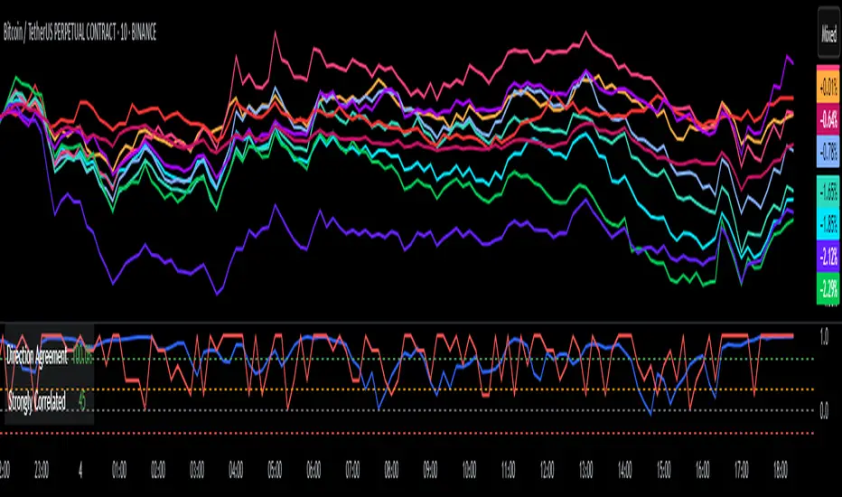
NY ORB + Fakeout Detector🗽 NY ORB + Fakeout Detector
This indicator automatically plots the New York Opening Range (ORB) based on the first 15 minutes of the NY session (15:30–15:45 CEST / 13:30–13:45 UTC) and detects potential fakeouts (false breakouts).
🔍 Key Features:
✅ Plots ORB high and low based on the 15-minute NY open range
✅ Automatically detects fake breakouts (price wicks beyond the box but closes back inside)
✅ Visual markers:
🔺 "Fake ↑" if a fake breakout occurs above the range
🔻 "Fake ↓" if a fake breakout occurs below the range
✅ Gray background highlights the ORB session window
✅ Designed for scalping and short-term breakout strategies
🧠 Best For:
Intraday traders looking for NY volatility setups
Scalpers using ORB-based entries
Traders seeking early-session fakeout traps to avoid false signals
Those combining with EMA 12/21, volume, or other confluence tools

Opening Range 15 minThis indicator highlights the Opening Range (OR) for the first 15 minutes (9:30–9:45 AM EST). It visually plots high/low lines and a shaded box to define this range, helping traders identify key intraday levels for potential breakout or rejection scenarios. The script also provides optional overlays for the Previous Day’s High/Low and the Extended Hours High/Low, offering a complete context for day trading setups.
Main Features:
Opening Range Detection – Automatically calculates and draws the high/low of the 9:30–9:45 AM session.
Visual Enhancements – Includes customizable lines, shaded boxes, and labels to mark the OR high (ORH) and low (ORL) levels.
Previous Day High/Low (Optional) – Plots and labels the previous day's high and low for reference during current day trading.
Extended Hours High/Low (Optional, when ETH enabled) – Displays overnight session levels for added insight into early volatility (4:00 AM to 9:30 AM EST).
User Customization – Easily adjust colors, label styles, and visibility for all plotted levels and regions.
Engulfing DetectorThis script detects classic candlestick reversal patterns known as Engulfing formations:
Bullish Engulfing: A green candle fully engulfs the previous red candle.
Bearish Engulfing: A red candle fully engulfs the previous green candle.
🔎 Features:
Works on any time frame or instrument.
Optional filter to ignore overly large or irregular candles.
Visual signals on the chart (BE/SE labels).
Built-in alerts for automation or notification.
✅ Recommended usage:
For intraday trading, this indicator performs best on the 5-minute chart of the Nasdaq (NQ) between 9:45 AM and 1:00 PM ET (15:45–19:00 CET).
💡 Suggested trading approach:
Optimized for scalping with short-term trades and small take-profits around +0.10%.

MFI + RSI + EMA Dynamic SignalsThe MFI + RSI + EMA Dynamic Signals is a designed to combine with widened criteria to capture more trading opportunities, it balances momentum, trend, and flexibility, making it suitable for trading on timeframes like 15-minute to 4-hour charts.
How It Works
The indicator uses three technical components with relaxed criteria to produce signals:
Money Flow Index (MFI) for Momentum Extremes:
The MFI, calculated over a 14-period length, measures buying and selling pressure using price and volume. A buy signal can trigger when MFI crosses above the oversold level (default: 30, widened from 20), indicating potential buying pressure, while a sell signal can occur when MFI crosses below the overbought level (default: 70, widened from 80), suggesting selling pressure.
Relative Strength Index (RSI) for Momentum Confirmation:
The RSI, calculated over a 14-period length, confirms momentum strength. Bullish momentum is confirmed when RSI is above a buy threshold (default: 45, relaxed from 50), and bearish momentum when below a sell threshold (default: 55, relaxed from 50), allowing more signals near neutral momentum levels.
Exponential Moving Average (EMA) for Trend Sensitivity:
The indicator uses a fast EMA (default: 9 periods) and a slow EMA (default: 21 periods) to detect trend direction and crossovers. Signals can trigger when the fast EMA crosses the slow EMA, or when the fast EMA is within a proximity threshold (default: 0.5%) of the slow EMA, capturing early trend changes and increasing signal frequency.
Signal Generation
Signals are generated using the previous bar’s values to prevent repainting, with widened criteria for more frequent triggers:
Buy Signal: Either the MFI crosses above the oversold level or the fast EMA crosses above the slow EMA, and either RSI confirms bullish momentum (above 45) or the EMAs are near a crossover (within 0.5%). Displayed as a green upward triangle below the bar.
Sell Signal: Either the MFI crosses below the overbought level or the fast EMA crosses below the slow EMA, and either RSI confirms bearish momentum (below 55) or the EMAs are near a crossover (within 0.5%). Displayed as a red downward triangle above the bar.

LANZ Strategy 2.0 [Backtest]🔷 LANZ Strategy 2.0 — Structural Breakout Logic with Dynamic Swing Protection
LANZ Strategy 2.0 is a precision-focused backtesting system built for intraday traders who rely on structural confirmations before the London session to guide directional bias. This tool uses smart swing detection, risk-defined position sizing, and strict time-based execution to simulate real trading conditions with clarity and control.
🧠 Core Components:
Structural Confirmation (Trend & BoS): Detects trend direction and break of structure (BoS) using a three-swing logic, aligning trade entries with valid structural movement.
Time-Based Execution: Trades are triggered exclusively at 02:00 a.m. New York time, ensuring disciplined and repeatable intraday testing.
Swing-Based SL Models: Traders can select between three stop-loss protection types:
First Swing: Most recent structural level
Second Swing: Prior level
Full Coverage: All recent swing levels + configurable pip buffer
Dynamic TP Calculation: Take-Profit is projected as a risk-based multiple (RR), fully adjustable via input.
Capital-Based Risk Management: Risk is defined as a percentage of a fixed account size (e.g., $100 per trade from $10,000), and lot size is automatically calculated based on SL distance.
Fallback Entry Logic: If structural breakout is present but trend is not confirmed, a secondary entry is triggered.
End-of-Session Management: Any open trades are automatically closed at 11:45 a.m. NY time, with optional manual labeling or review.
📊 Visual Features (Optional in Indicator Version):
(Note: Visuals apply to the indicator version of LANZ 2.0, not this backtest script)
Swing level labels (1st, 2nd) and dynamic SL/TP lines.
Real-time session coloring for clarity: Pre-London, Entry Window, and NY Close.
Outcome labels: +RR, -RR, or net % at close.
Auto-cleanup of previous drawings for a clean chart per session.
⚙️ How It Works:
Detects last trend and BoS using swing logic before 02:00 a.m. NY.
At 02:00 a.m., evaluates directional bias and executes BUY or SELL if confirmed.
Applies selected SL logic (1st, 2nd, or full swing protection).
Sets TP based on the RR multiplier.
Closes the trade either on SL, TP, or at 11:45 a.m. NY manually.
🔔 Alerts:
Time-of-day alert at 02:00 a.m. NY to monitor execution.
Can be extended to cover SL/TP triggers or new BoS events.
📝 Notes:
Designed for backtesting precision and discretionary decision-making.
Ideal for Forex pairs, indices, or assets active during the London session.
Fully customizable: session timing, swing logic, SL buffer, and RR.
👤 Credits:
Strategy built by @rau_u_lanz using Pine Script v6, combining structural logic, capital-based risk control, and London-session timing in a backtest-ready framework for traders who demand accuracy and structure.

RVOL - Relative Volume IntradayIn the context of intraday trading, RVOL stands for Relative Volume. It is a technical indicator that compares the current volume of a stock to its average volume over a specified period. A RVOL above 1 suggests higher than average trading volume, potentially indicating increased interest and volatility.
The precise definition of real time relative volume is current cumulative volume up to the time of day divided by average cumulative volume up to this time of day. It means for example taking the volume from 09:45 to 10:00 and comparing it to what it does from 09:45 to 10:00 every day.
This indicator supports all timeframes from1 minute to 4 hours.
ORB-HL1. Opening Range Detection
Automatically calculates the high and low of the first 15 minutes after the selected session opens.
Supported sessions:
New York (Futures): 08:30–08:45 EST
New York (Equities): 09:30–09:45 EST
London: 03:00–03:15 GMT
Asia: 19:00–19:15 JST
Plots ORB high/low lines for the rest of the day.
2. Breakout Signals
Highlights the first valid breakout above or below the ORB range on the:
5-minute timeframe
15-minute timeframe
Green arrows = breakout up (long)
Red arrows = breakout down (short)
3. 1-Minute Projection
When a breakout is confirmed on a higher timeframe (5m or 15m), a projection label (e.g., "5m", "15m") appears on the 1-minute chart.
Purple label = 5m breakout
Teal label = 15m breakout
Helps you confirm momentum in real time while on the 1-minute chart.
4. Trailing Stop System
Uses ATR to create an adaptive trailing stop after breakout.
Turns green when price is above stop (bullish), red when below (bearish).
Optional Buy / Sell signal labels appear on crossover events.
5. Session High/Low Visualization
Tracks and displays the previous session’s High and Low for:
Tokyo
London
New York
Lines extend into the current session to act as S/R reference.
Labels like "NY High", "Asia Low" are placed at the end of each line.
6. Alerts
Built-in alerts for:
First 5m or 15m breakout (long/short)
Trailing stop Buy/Sell crossover
7. Customization Options
Turn session H/L lines on/off per session
Customize projection visibility
Adjust ATR period and sensitivity
Set how far each session line extends using bar offsets

LANZ Strategy 2.0🔷 LANZ Strategy 2.0 — London Breakout Confirmation with Structural Swing Protection
LANZ Strategy 2.0 is a structured trading system that leverages the last confirmed market direction before the London session to define directional bias and manage trades based on key structural swing levels. It is tailored for intraday traders looking to capitalize on early London volatility with built-in risk management and visual clarity.
🧠 Core Components:
Directional Confirmation (Pre-London Bias): Validates the last breakout or structural move from the 15-minute timeframe before 02:15 a.m. New York time (start of the London session), establishing the expected market direction.
Time-Based Execution: Executes potential entries strictly at 02:15 a.m. NY time, using market structure to support Long or Short bias.
Dynamic Swing-Based SL System: Allows user to select between three SL protection models: First Swing (most recent structural point) Second Swing (prior level) Total Coverage (includes both swings + extra buffer) This supports flexibility based on trader profile or market conditions.
Visual Risk Mapping: All SL and TP levels are clearly plotted.
End-of-Session Management: Positions are automatically evaluated for closure at 11:45 a.m. NY time. SL, TP, or manual close outcomes are labeled accordingly.
📊 Visual Features:
Labels for 1st and 2nd swing levels upon entry.
Dynamic lines projecting SL/TP levels toward the end of the session.
Session background coloring for Pre-London, Execution, and NY sessions.
Real-time percentage outcome labels (+2.00%, -1.00%, or net % at session end).
Automatic deletion of previous visuals on new entries for clean charting.
⚙️ How It Works:
Detects last structural breakout on the 15m timeframe before 02:15 a.m. NY.
On the 02:15 a.m. candle, executes a Long or Short logic entry.
Plots corresponding SL and TP based on selected swing model.
Monitors price action: If TP or SL is hit, labels it accordingly. If no exit is hit, trade closes manually at 11:45 a.m. NY with net result shown.
Optional logic to reverse entries if market structure breaks before execution.
🔔 Alerts:
Daily execution alert at 02:15 a.m. NY (prompting manual review or action).
Optional alert logic can be extended for SL/TP hits or structure breaks.
📝 Notes:
Designed for semi-automated or discretionary intraday trading.
Best used on Forex pairs or indices with strong London session behavior.
Adjustable parameters include session hours, swing SL type, and buffer settings.
Credits:
Developed by LANZ, this script combines time-based execution with dynamic structure protection, offering a disciplined framework for participating in the London session breakout with clear visuals and risk logic.

ICT Macro and Daye QT ShiftEST Vertical Lines - Auto DST Adjustment
Overview
This indicator draws customizable vertical lines at specific Eastern Time (EST/EDT) points throughout the trading day, automatically adjusting for daylight savings time. Designed for precision trading on 1-minute and 5-minute charts, it highlights key intraday moments when price action tends to accelerate.
Features
- **18 pre-configured NY session times** (09:50-15:45 ET)
- **Auto timezone conversion** - Always shows correct EST/EDT regardless of your local timezone
- **3 line styles** - Choose between solid/dashed/dotted lines
- **Clean labeling** - Optional time markers above each line
- **1m/5m optimized** - Perfect for scalpers and day traders
- **Visual alerts** - "TOUCH" labels when price interacts with lines
Inputs
| Parameter | Description | Default |
|-----------|-------------|---------|
| Line Times | Comma-separated HH:MM times | 09:50,10:10,...15:45 |
| Line Color | Line color | Black |
| Line Width | 1-5px thickness | 2 |
| Line Style | Solid/Dashed/Dotted | Solid |
| Show Labels | Display time markers | true |
How To Use
1. Apply to 1m or 5m charts
2. Lines appear automatically at specified EST times
3. Watch for price reactions at these key levels
4. Customize styles via indicator settings
Ideal For
- NY open/London close traders
- Earnings/News traders
- Breakout traders
- Market open/close strategies
Updates
v1.1 - Added line style customization
v1.0 - Initial release
