EMD Oscillator (Zeiierman)█ Overview
The Empirical Mode Decomposition (EMD) Oscillator is an advanced indicator designed to analyze market trends and cycles with high precision. It breaks down complex price data into simpler parts called Intrinsic Mode Functions (IMFs), allowing traders to see underlying patterns and trends that aren’t visible with traditional indicators. The result is a dynamic oscillator that provides insights into overbought and oversold conditions, as well as trend direction and strength. This indicator is suitable for all types of traders, from beginners to advanced, looking to gain deeper insights into market behavior.
█ How It Works
The core of this indicator is the Empirical Mode Decomposition (EMD) process, a method typically used in signal processing and advanced scientific fields. It works by breaking down price data into various “layers,” each representing different frequencies in the market’s movement. Imagine peeling layers off an onion: each layer (or IMF) reveals a different aspect of the price action.
⚪ Data Decomposition (Sifting): The indicator “sifts” through historical price data to detect natural oscillations within it. Each oscillation (or IMF) highlights a unique rhythm in price behavior, from rapid fluctuations to broader, slower trends.
⚪ Adaptive Signal Reconstruction: The EMD Oscillator allows traders to select specific IMFs for a custom signal reconstruction. This reconstructed signal provides a composite view of market behavior, showing both short-term cycles and long-term trends based on which IMFs are included.
⚪ Normalization: To make the oscillator easy to interpret, the reconstructed signal is scaled between -1 and 1. This normalization lets traders quickly spot overbought and oversold conditions, as well as trend direction, without worrying about the raw magnitude of price changes.
The indicator adapts to changing market conditions, making it effective for identifying real-time market cycles and potential turning points.
█ Key Calculations: The Math Behind the EMD Oscillator
The EMD Oscillator’s advanced nature lies in its high-level mathematical operations:
⚪ Intrinsic Mode Functions (IMFs)
IMFs are extracted from the data and act as the building blocks of this indicator. Each IMF is a unique oscillation within the price data, similar to how a band might be divided into treble, mid, and bass frequencies. In the EMD Oscillator:
Higher-Frequency IMFs: Represent short-term market “noise” and quick fluctuations.
Lower-Frequency IMFs: Capture broader market trends, showing more stable and long-term patterns.
⚪ Sifting Process: The Heart of EMD
The sifting process isolates each IMF by repeatedly separating and refining the data. Think of this as filtering water through finer and finer mesh sieves until only the clearest parts remain. Mathematically, it involves:
Extrema Detection: Finding all peaks and troughs (local maxima and minima) in the data.
Envelope Calculation: Smoothing these peaks and troughs into upper and lower envelopes using cubic spline interpolation (a method for creating smooth curves between data points).
Mean Removal: Calculating the average between these envelopes and subtracting it from the data to isolate one IMF. This process repeats until the IMF criteria are met, resulting in a clean oscillation without trend influences.
⚪ Spline Interpolation
The cubic spline interpolation is an advanced mathematical technique that allows smooth curves between points, which is essential for creating the upper and lower envelopes around each IMF. This interpolation solves a tridiagonal matrix (a specialized mathematical problem) to ensure that the envelopes align smoothly with the data’s natural oscillations.
To give a relatable example: imagine drawing a smooth line that passes through each peak and trough of a mountain range on a map. Spline interpolation ensures that line is as smooth and close to reality as possible. Achieving this in Pine Script is technically demanding and demonstrates a high level of mathematical coding.
⚪ Amplitude Normalization
To make the oscillator more readable, the final signal is scaled by its maximum amplitude. This amplitude normalization brings the oscillator into a range of -1 to 1, creating consistent signals regardless of price level or volatility.
█ Comparison with Other Signal Processing Methods
Unlike standard technical indicators that often rely on fixed parameters or pre-defined mathematical functions, the EMD adapts to the data itself, capturing natural cycles and irregularities in real-time. For example, if the market becomes more volatile, EMD adjusts automatically to reflect this without requiring parameter changes from the trader. In this way, it behaves more like a “smart” indicator, intuitively adapting to the market, unlike most traditional methods. EMD’s adaptive approach is akin to AI’s ability to learn from data, making it both resilient and robust in non-linear markets. This makes it a great alternative to methods that struggle in volatile environments, such as fixed-parameter oscillators or moving averages.
█ How to Use
Identify Market Cycles and Trends: Use the EMD Oscillator to spot market cycles that represent phases of buying or selling pressure. The smoothed version of the oscillator can help highlight broader trends, while the main oscillator reveals immediate cycles.
Spot Overbought and Oversold Levels: When the oscillator approaches +1 or -1, it may indicate that the market is overbought or oversold, signaling potential entry or exit points.
Confirm Divergences: If the price movement diverges from the oscillator's direction, it may indicate a potential reversal. For example, if prices make higher highs while the oscillator makes lower highs, it could be a sign of weakening trend strength.
█ Settings
Window Length (N): Defines the number of historical bars used for EMD analysis. A larger window captures more data but may slow down performance.
Number of IMFs (M): Sets how many IMFs to extract. Higher values allow for a more detailed decomposition, isolating smaller cycles within the data.
Amplitude Window (L): Controls the length of the window used for amplitude calculation, affecting the smoothness of the normalized oscillator.
Extraction Range (IMF Start and End): Allows you to select which IMFs to include in the reconstructed signal. Starting with lower IMFs captures faster cycles, while ending with higher IMFs includes slower, trend-based components.
Sifting Stopping Criterion (S-number): Sets how precisely each IMF should be refined. Higher values yield more accurate IMFs but take longer to compute.
Max Sifting Iterations (num_siftings): Limits the number of sifting iterations for each IMF extraction, balancing between performance and accuracy.
Source: The price data used for the analysis, such as close or open prices. This determines which price movements are decomposed by the indicator.
-----------------
Disclaimer
The information contained in my Scripts/Indicators/Ideas/Algos/Systems does not constitute financial advice or a solicitation to buy or sell any securities of any type. I will not accept liability for any loss or damage, including without limitation any loss of profit, which may arise directly or indirectly from the use of or reliance on such information.
All investments involve risk, and the past performance of a security, industry, sector, market, financial product, trading strategy, backtest, or individual's trading does not guarantee future results or returns. Investors are fully responsible for any investment decisions they make. Such decisions should be based solely on an evaluation of their financial circumstances, investment objectives, risk tolerance, and liquidity needs.
My Scripts/Indicators/Ideas/Algos/Systems are only for educational purposes!
Pine Script®指标