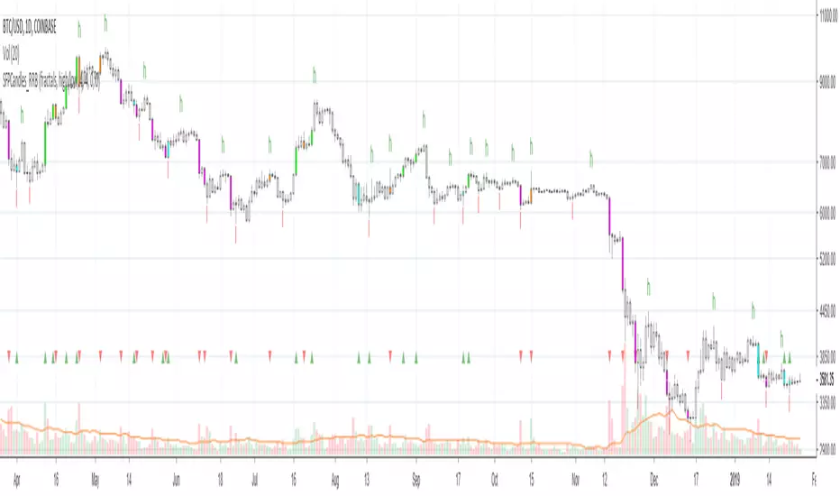
Kawabunga Swing Failure Points Candles (SFP) by RRBKawabunga Swing Failure Points Candles (SFP) by RagingRocketBull 2019
Version 1.0
This indicator shows Swing Failure Points (SFP) and Swing Confirmation Points (SCP) as candles on a chart.
SFP/SCP candles are used by traders as signals for trend confirmation/possible reversal.
The signal is stronger on a higher volume/larger candle size.
A Swing Failure Point (SFP) candle is used to spot a reversal:
- up trend SFP is a failure to close above prev high after making a new higher high => implies reversal down
- down trend SFP is a failure to close below prev low after making a new lower low => implies reversal up
A Swing Confirmation Point (SCP) candle is just the opposite and is used to confirm the current trend:
- up trend SCP is a successful close above prev high after making a new higher high => confirms the trend and implies continuation up
- down trend SCP is a successful close below prev low after making a new lower low => confirms the trend and implies continuation down
Features:
- uses fractal pivots with optional filter
- show/hide SFP/SCP candles, pivots, zigzag, last min/max pivot bands
- dim lag zones/hide false signals introduced by lagging fractals or
- use unconfirmed pivots to eliminate fractal lag/false signals. 2 modes: fractals 1,1 and highest/lowest
- filter only SFP/SCP candles confirmed with volume/candle size
- SFP/SCP candles color highlighting, dim non-important bars
Usage:
- adjust fractal settings to get pivots that best match your data (lower values => more frequent pivots. 0,0 - each candle is a pivot)
- use one of the unconfirmed pivot modes to eliminate false signals or just ignore all signals in the gray lag zones
- optionally filter only SFP/SCP candles with large volume/candle size (volume % change relative to prev bar, abs candle body size value)
- up/down trend SCP (lime/fuchsia) => continuation up/down; up/down trend SFP (orange/aqua) => possible reversal down/up. lime/aqua => up; fuchsia/orange => down.
- when in doubt use show/hide pivots/unconfirmed pivots, min/max pivot bands to see which prev pivot and min/max value were used in comparisons to generate a signal on the following candle.
- disable offset to check on which bar the signal was generated
Notes:
Fractal Pivots:
- SFP/SCP candles depend on fractal pivots, you will get different signals with different pivot settings. Usually 4,4 or 2,2 settings are used to produce fractal pivots, but you can try custom values that fit your data best.
- fractal pivots are a mixed series of highs and lows in no particular order. Pivots must be filtered to produce a proper zigzag where ideally a high is followed by a low and another high in orderly fashion.
Fractal Lag/False Signals:
- only past fractal pivots can be processed on the current bar introducing a lag, therefore, pivots and min/max pivot bands are shown with offset=-rightBars to match their target bars. For unconfirmed pivots an offset=-1 is used with a lag of just 1 bar.
- new pivot is not a confirmed fractal and "does not exist yet" while the distance between it and the current bar is < rightBars => prev old fractal pivot in the same dir is used for comparisons => gives a false signal for that dir
- to show false signals enable lag zones. SFP/SCP candles in lag zones are false. New pivots will be eventually confirmed, but meanwhile you get a false signal because prev pivot in the same dir was used instead.
- to solve this problem you can either temporary hide false signals or completely eliminate them by using unconfirmed pivots of a smaller degree/lag.
- hiding false signals only works for history and should be used only temporary (left disabled). In realtime/replay mode it disables all signals altogether due to TradingView's bug (barcolor doesn't support negative offsets)
Unconfirmed Pivots:
- you have 2 methods to check for unconfirmed pivots: highest/lowest(rightBars) or fractals(1,1) with a min possible step. The first is essentially fractals(0,0) where each candle is a pivot. Both produce more frequent pivots (weaker signals).
- an unconfirmed pivot is used in comparisons to generate a valid signal only when it is a higher high (> max high) or a lower low (< min low) in the dir of a trend. Confirmed pivots of a higher degree are not affected. Zigzag is not affected.
- you can also manually disable the offset to check on which bar the pivot was confirmed. If the pivot just before an SCP/SFP suddenly jumps ahead of it - prev pivot was used, generating a false signal.
- last max high/min low bands can be used to check which value was used in candle comparison to generate a signal: min(pivot min_low, upivot min_low) and max(pivot max_high, upivot max_high) are used
- in the unconfirmed pivots mode the max high/min low pivot bands partially break because you can't have a variable offset to match the random pos of an unconfirmed pivot (anywhere in 0..rightBars from the current bar) to its target bar.
- in the unconfirmed pivots mode h (green) and l (red) pivots become H and L, and h (lime) and l (fuchsia) are used to show unconfirmed pivots of a smaller degree. Some of them will be confirmed later as H and L pivots of a higher degree.
Pivot Filter:
- pivot filter is used to produce a better looking zigzag. Essentially it keeps only higher highs/lower lows in the trend direction until it changes, skipping:
- after a new high: all subsequent lower highs until a new low
- after a new low: all subsequent higher lows until a new high
- you can't filter out all prev highs/lows to keep just the last min/max pivots of the current swing because they were already confirmed as pivots and you can't delete/change history
- alternatively you could just pick the first high following a low and the first low following a high in a sequence and ignore the rest of the pivots in the same dir, producing a crude looking zigzag where obvious max high/min lows are ignored.
- pivot filter affects SCP/SFP signals because it skips some pivots
- pivot filter is not applied to/not affected by the unconfirmed pivots
- zigzag is affected by pivot filter, but not by the unconfirmed pivots. You can't have both high/low on the same bar in a zigzag. High has priority over Low.
- keep same bar pivots option lets you choose which pivots to keep when there are both high/low pivots on the same bar (both kept by default)
SCP/SFP Filters:
- you can confirm/filter only SCP/SFP signals with volume % change/candle size larger than delta. Higher volume/larger candle means stronger signal.
- technically SCP/SFP is always the first matching candle, but it can be invalidated by the following signal in the opposite dir which in turn can be negated by the next signal.
- show first matching SCP/SFP = true - shows only the first signal candle (and any invalidations that follow) and hides further duplicate signals in the same dir, does not highlight the trend.
- show first matching SCP/SFP = false - produces a sequence of candles with duplicate signals, highlights the whole trend until its dir changes (new pivot).
Good Luck! Feel free to learn from/reuse the code to build your own indicators!
在脚本中搜索"Fractal"
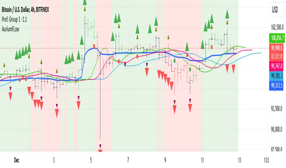
AuriumFlowAURIUM (GOLD-Weighted Average with Fractal Dynamics)
Aurium is a cutting-edge indicator that blends volume-weighted moving averages (VWMA), fractal geometry, and Fibonacci-inspired calculations to deliver a precise and holistic view of market trends. By dynamically adjusting to price and volume, Aurium uncovers key levels of confluence for trend reversals and continuations, making it a powerful tool for traders.
Key Features:
Dynamic Trendline (GOLD):
The central trendline is a weighted moving average based on price and volume, tuned using Fibonacci-based fast (34) and slow (144) exponential moving average lengths. This ensures the trendline adapts seamlessly to the flow of market dynamics.
Formula:
GOLD = VWMA(34) * Volume Factor + VWMA(144) * (1 - Volume Factor)
Fractal Highs and Lows:
Detects pivotal market points using a fractal lookback period (default 5, odd-numbered). Fractals identify local highs and lows over a defined window, capturing the structure of market cycles.
Trend Background Highlighting:
Bullish Zone: Price above the GOLD line with a green background.
Bearish Zone: Price below the GOLD line with a red background.
Buy and Sell Alerts:
Generates actionable signals when fractals align with GOLD. Bullish fractals confirm continuation or reversal in an uptrend, while bearish fractals validate a downtrend.
The Math Behind Aurium:
Volume-Weighted Adjustments:
By integrating volume into the calculation, Aurium dynamically emphasizes price levels with greater participation, giving traders insight into zones of institutional interest.
Formula:
VWMA = EMA(Close * Volume) / EMA(Volume)
Fractal Calculations:
Fractals are identified as local maxima (highs) or minima (lows) based on the surrounding bars, leveraging the natural symmetry in price behavior.
Fibonacci Relationships:
The 34 and 144 EMA lengths are Fibonacci numbers, offering a natural alignment with price cycles and market rhythms.
Ideal For:
Traders seeking a precise and intuitive indicator for aligning with trends and detecting reversals.
Strategies inspired by Bill Williams, with added volume and fractal-based insights.
Short-term scalpers and long-term trend-followers alike.
Unlock deeper market insights and trade with precision using Aurium!
MSSM - Multi-Session Structural Map (Precision Sweeps)MSSM – Multi-Session Structural Map (Precision Sweeps)
This indicator provides a structured view of the market based on four key components:
1). Previous session levels
2). Confirmed fractal swing points
3). Volume pocket highlights
4). Non-repainting precision liquidity sweep markers
It is designed to help analyze how price interacts with important reference areas and structural points. This tool does not generate signals or predictions. All information is visual and educational only.
HOW THE INDICATOR WORKS
PREVIOUS SESSION LEVELS
The script plots the previous session’s High, Low, and Mid. These levels help observe how the current session behaves around the prior day’s range. They act as reference areas only.
FRACTAL SWING MAP (NON-REPAINTING)
Confirmed fractals are used to mark historical swing highs and swing lows. Since fractals confirm after a certain number of bars, the swings do not repaint once formed. These swings provide a clearer view of market structure.
VOLUME POCKETS
The indicator highlights areas where volume expands relative to a rolling volume average. These regions show increased participation or activity. The highlights are informational and do not imply direction.
PRECISION LIQUIDITY SWEEPS (NON-REPAINTING)
A sweep is tagged only when:
• Price trades beyond a confirmed swing high or swing low
• Price closes back inside the previous swing level
• A wick rejection occurs
• Volume expands relative to a recent rolling average
These markers simply show where price interacted with liquidity around prior structural levels. They do not indicate a trading signal or bias.
HOW TO ADD THE INDICATOR
Open the Pine Editor in TradingView
Search the indicator name and add to favorites.
Click “Add to chart”
Adjust settings as needed (fractals, sweeps, volume pockets, or session levels)
HOW TO READ AND USE THE INDICATOR
SESSION LEVELS
Observe whether price respects, rejects, compresses around, or expands beyond the previous session high, low, or midpoint. These are observational reference levels only.
FRACTALS
Fractal highs and lows help visualize structural turning points. They provide a clearer picture of where liquidity may rest above or below past swing levels.
VOLUME POCKETS
When volume expands compared to the recent average, the candle is shaded. These areas may show increased participation, but no directional meaning is implied.
PRECISION SWEEPS
Sweeps highlight when price reaches beyond a prior confirmed swing level and then rejects that area with displacement. These markers identify interactions with liquidity, but they are not signals and do not forecast future outcomes.
CUSTOMIZATION OPTIONS
Users can adjust:
• Session level visibility
• Fractal sensitivity
• Volume pocket threshold
• Sweep sensitivity and visibility
• Transparency and styling
This makes the tool flexible across different symbols and timeframes.
IMPORTANT NOTES AND POLICY COMPLIANCE
• The indicator does not provide buy or sell signals
• The indicator does not predict price or direction
• All plotted elements are based on past price behavior
• All components are informational only
• Users should perform their own analysis and risk evaluation
• Past behavior does not guarantee future performance
SUMMARY
MSSM provides a structured view of price by combining previous session levels, confirmed swing structure, volume expansion zones, and non-repainting sweep identification. Its purpose is to assist traders in visually analyzing market structure while staying fully aligned with TradingView’s House Rules and content policies.

Dimensional Resonance ProtocolDimensional Resonance Protocol
🌀 CORE INNOVATION: PHASE SPACE RECONSTRUCTION & EMERGENCE DETECTION
The Dimensional Resonance Protocol represents a paradigm shift from traditional technical analysis to complexity science. Rather than measuring price levels or indicator crossovers, DRP reconstructs the hidden attractor governing market dynamics using Takens' embedding theorem, then detects emergence —the rare moments when multiple dimensions of market behavior spontaneously synchronize into coherent, predictable states.
The Complexity Hypothesis:
Markets are not simple oscillators or random walks—they are complex adaptive systems existing in high-dimensional phase space. Traditional indicators see only shadows (one-dimensional projections) of this higher-dimensional reality. DRP reconstructs the full phase space using time-delay embedding, revealing the true structure of market dynamics.
Takens' Embedding Theorem (1981):
A profound mathematical result from dynamical systems theory: Given a time series from a complex system, we can reconstruct its full phase space by creating delayed copies of the observation.
Mathematical Foundation:
From single observable x(t), create embedding vectors:
X(t) =
Where:
• d = Embedding dimension (default 5)
• τ = Time delay (default 3 bars)
• x(t) = Price or return at time t
Key Insight: If d ≥ 2D+1 (where D is the true attractor dimension), this embedding is topologically equivalent to the actual system dynamics. We've reconstructed the hidden attractor from a single price series.
Why This Matters:
Markets appear random in one dimension (price chart). But in reconstructed phase space, structure emerges—attractors, limit cycles, strange attractors. When we identify these structures, we can detect:
• Stable regions : Predictable behavior (trade opportunities)
• Chaotic regions : Unpredictable behavior (avoid trading)
• Critical transitions : Phase changes between regimes
Phase Space Magnitude Calculation:
phase_magnitude = sqrt(Σ ² for i = 0 to d-1)
This measures the "energy" or "momentum" of the market trajectory through phase space. High magnitude = strong directional move. Low magnitude = consolidation.
📊 RECURRENCE QUANTIFICATION ANALYSIS (RQA)
Once phase space is reconstructed, we analyze its recurrence structure —when does the system return near previous states?
Recurrence Plot Foundation:
A recurrence occurs when two phase space points are closer than threshold ε:
R(i,j) = 1 if ||X(i) - X(j)|| < ε, else 0
This creates a binary matrix showing when the system revisits similar states.
Key RQA Metrics:
1. Recurrence Rate (RR):
RR = (Number of recurrent points) / (Total possible pairs)
• RR near 0: System never repeats (highly stochastic)
• RR = 0.1-0.3: Moderate recurrence (tradeable patterns)
• RR > 0.5: System stuck in attractor (ranging market)
• RR near 1: System frozen (no dynamics)
Interpretation: Moderate recurrence is optimal —patterns exist but market isn't stuck.
2. Determinism (DET):
Measures what fraction of recurrences form diagonal structures in the recurrence plot. Diagonals indicate deterministic evolution (trajectory follows predictable paths).
DET = (Recurrence points on diagonals) / (Total recurrence points)
• DET < 0.3: Random dynamics
• DET = 0.3-0.7: Moderate determinism (patterns with noise)
• DET > 0.7: Strong determinism (technical patterns reliable)
Trading Implication: Signals are prioritized when DET > 0.3 (deterministic state) and RR is moderate (not stuck).
Threshold Selection (ε):
Default ε = 0.10 × std_dev means two states are "recurrent" if within 10% of a standard deviation. This is tight enough to require genuine similarity but loose enough to find patterns.
🔬 PERMUTATION ENTROPY: COMPLEXITY MEASUREMENT
Permutation entropy measures the complexity of a time series by analyzing the distribution of ordinal patterns.
Algorithm (Bandt & Pompe, 2002):
1. Take overlapping windows of length n (default n=4)
2. For each window, record the rank order pattern
Example: → pattern (ranks from lowest to highest)
3. Count frequency of each possible pattern
4. Calculate Shannon entropy of pattern distribution
Mathematical Formula:
H_perm = -Σ p(π) · ln(p(π))
Where π ranges over all n! possible permutations, p(π) is the probability of pattern π.
Normalized to :
H_norm = H_perm / ln(n!)
Interpretation:
• H < 0.3 : Very ordered, crystalline structure (strong trending)
• H = 0.3-0.5 : Ordered regime (tradeable with patterns)
• H = 0.5-0.7 : Moderate complexity (mixed conditions)
• H = 0.7-0.85 : Complex dynamics (challenging to trade)
• H > 0.85 : Maximum entropy (nearly random, avoid)
Entropy Regime Classification:
DRP classifies markets into five entropy regimes:
• CRYSTALLINE (H < 0.3): Maximum order, persistent trends
• ORDERED (H < 0.5): Clear patterns, momentum strategies work
• MODERATE (H < 0.7): Mixed dynamics, adaptive required
• COMPLEX (H < 0.85): High entropy, mean reversion better
• CHAOTIC (H ≥ 0.85): Near-random, minimize trading
Why Permutation Entropy?
Unlike traditional entropy methods requiring binning continuous data (losing information), permutation entropy:
• Works directly on time series
• Robust to monotonic transformations
• Computationally efficient
• Captures temporal structure, not just distribution
• Immune to outliers (uses ranks, not values)
⚡ LYAPUNOV EXPONENT: CHAOS vs STABILITY
The Lyapunov exponent λ measures sensitivity to initial conditions —the hallmark of chaos.
Physical Meaning:
Two trajectories starting infinitely close will diverge at exponential rate e^(λt):
Distance(t) ≈ Distance(0) × e^(λt)
Interpretation:
• λ > 0 : Positive Lyapunov exponent = CHAOS
- Small errors grow exponentially
- Long-term prediction impossible
- System is sensitive, unpredictable
- AVOID TRADING
• λ ≈ 0 : Near-zero = CRITICAL STATE
- Edge of chaos
- Transition zone between order and disorder
- Moderate predictability
- PROCEED WITH CAUTION
• λ < 0 : Negative Lyapunov exponent = STABLE
- Small errors decay
- Trajectories converge
- System is predictable
- OPTIMAL FOR TRADING
Estimation Method:
DRP estimates λ by tracking how quickly nearby states diverge over a rolling window (default 20 bars):
For each bar i in window:
δ₀ = |x - x | (initial separation)
δ₁ = |x - x | (previous separation)
if δ₁ > 0:
ratio = δ₀ / δ₁
log_ratios += ln(ratio)
λ ≈ average(log_ratios)
Stability Classification:
• STABLE : λ < 0 (negative growth rate)
• CRITICAL : |λ| < 0.1 (near neutral)
• CHAOTIC : λ > 0.2 (strong positive growth)
Signal Filtering:
By default, NEXUS requires λ < 0 (stable regime) for signal confirmation. This filters out trades during chaotic periods when technical patterns break down.
📐 HIGUCHI FRACTAL DIMENSION
Fractal dimension measures self-similarity and complexity of the price trajectory.
Theoretical Background:
A curve's fractal dimension D ranges from 1 (smooth line) to 2 (space-filling curve):
• D ≈ 1.0 : Smooth, persistent trending
• D ≈ 1.5 : Random walk (Brownian motion)
• D ≈ 2.0 : Highly irregular, space-filling
Higuchi Method (1988):
For a time series of length N, construct k different curves by taking every k-th point:
L(k) = (1/k) × Σ|x - x | × (N-1)/(⌊(N-m)/k⌋ × k)
For different values of k (1 to k_max), calculate L(k). The fractal dimension is the slope of log(L(k)) vs log(1/k):
D = slope of log(L) vs log(1/k)
Market Interpretation:
• D < 1.35 : Strong trending, persistent (Hurst > 0.5)
- TRENDING regime
- Momentum strategies favored
- Breakouts likely to continue
• D = 1.35-1.45 : Moderate persistence
- PERSISTENT regime
- Trend-following with caution
- Patterns have meaning
• D = 1.45-1.55 : Random walk territory
- RANDOM regime
- Efficiency hypothesis holds
- Technical analysis least reliable
• D = 1.55-1.65 : Anti-persistent (mean-reverting)
- ANTI-PERSISTENT regime
- Oscillator strategies work
- Overbought/oversold meaningful
• D > 1.65 : Highly complex, choppy
- COMPLEX regime
- Avoid directional bets
- Wait for regime change
Signal Filtering:
Resonance signals (secondary signal type) require D < 1.5, indicating trending or persistent dynamics where momentum has meaning.
🔗 TRANSFER ENTROPY: CAUSAL INFORMATION FLOW
Transfer entropy measures directed causal influence between time series—not just correlation, but actual information transfer.
Schreiber's Definition (2000):
Transfer entropy from X to Y measures how much knowing X's past reduces uncertainty about Y's future:
TE(X→Y) = H(Y_future | Y_past) - H(Y_future | Y_past, X_past)
Where H is Shannon entropy.
Key Properties:
1. Directional : TE(X→Y) ≠ TE(Y→X) in general
2. Non-linear : Detects complex causal relationships
3. Model-free : No assumptions about functional form
4. Lag-independent : Captures delayed causal effects
Three Causal Flows Measured:
1. Volume → Price (TE_V→P):
Measures how much volume patterns predict price changes.
• TE > 0 : Volume provides predictive information about price
- Institutional participation driving moves
- Volume confirms direction
- High reliability
• TE ≈ 0 : No causal flow (weak volume/price relationship)
- Volume uninformative
- Caution on signals
• TE < 0 (rare): Suggests price leading volume
- Potentially manipulated or thin market
2. Volatility → Momentum (TE_σ→M):
Does volatility expansion predict momentum changes?
• Positive TE : Volatility precedes momentum shifts
- Breakout dynamics
- Regime transitions
3. Structure → Price (TE_S→P):
Do support/resistance patterns causally influence price?
• Positive TE : Structural levels have causal impact
- Technical levels matter
- Market respects structure
Net Causal Flow:
Net_Flow = TE_V→P + 0.5·TE_σ→M + TE_S→P
• Net > +0.1 : Bullish causal structure
• Net < -0.1 : Bearish causal structure
• |Net| < 0.1 : Neutral/unclear causation
Causal Gate:
For signal confirmation, NEXUS requires:
• Buy signals : TE_V→P > 0 AND Net_Flow > 0.05
• Sell signals : TE_V→P > 0 AND Net_Flow < -0.05
This ensures volume is actually driving price (causal support exists), not just correlated noise.
Implementation Note:
Computing true transfer entropy requires discretizing continuous data into bins (default 6 bins) and estimating joint probability distributions. NEXUS uses a hybrid approach combining TE theory with autocorrelation structure and lagged cross-correlation to approximate information transfer in computationally efficient manner.
🌊 HILBERT PHASE COHERENCE
Phase coherence measures synchronization across market dimensions using Hilbert transform analysis.
Hilbert Transform Theory:
For a signal x(t), the Hilbert transform H (t) creates an analytic signal:
z(t) = x(t) + i·H (t) = A(t)·e^(iφ(t))
Where:
• A(t) = Instantaneous amplitude
• φ(t) = Instantaneous phase
Instantaneous Phase:
φ(t) = arctan(H (t) / x(t))
The phase represents where the signal is in its natural cycle—analogous to position on a unit circle.
Four Dimensions Analyzed:
1. Momentum Phase : Phase of price rate-of-change
2. Volume Phase : Phase of volume intensity
3. Volatility Phase : Phase of ATR cycles
4. Structure Phase : Phase of position within range
Phase Locking Value (PLV):
For two signals with phases φ₁(t) and φ₂(t), PLV measures phase synchronization:
PLV = |⟨e^(i(φ₁(t) - φ₂(t)))⟩|
Where ⟨·⟩ is time average over window.
Interpretation:
• PLV = 0 : Completely random phase relationship (no synchronization)
• PLV = 0.5 : Moderate phase locking
• PLV = 1 : Perfect synchronization (phases locked)
Pairwise PLV Calculations:
• PLV_momentum-volume : Are momentum and volume cycles synchronized?
• PLV_momentum-structure : Are momentum cycles aligned with structure?
• PLV_volume-structure : Are volume and structural patterns in phase?
Overall Phase Coherence:
Coherence = (PLV_mom-vol + PLV_mom-struct + PLV_vol-struct) / 3
Signal Confirmation:
Emergence signals require coherence ≥ threshold (default 0.70):
• Below 0.70: Dimensions not synchronized, no coherent market state
• Above 0.70: Dimensions in phase, coherent behavior emerging
Coherence Direction:
The summed phase angles indicate whether synchronized dimensions point bullish or bearish:
Direction = sin(φ_momentum) + 0.5·sin(φ_volume) + 0.5·sin(φ_structure)
• Direction > 0 : Phases pointing upward (bullish synchronization)
• Direction < 0 : Phases pointing downward (bearish synchronization)
🌀 EMERGENCE SCORE: MULTI-DIMENSIONAL ALIGNMENT
The emergence score aggregates all complexity metrics into a single 0-1 value representing market coherence.
Eight Components with Weights:
1. Phase Coherence (20%):
Direct contribution: coherence × 0.20
Measures dimensional synchronization.
2. Entropy Regime (15%):
Contribution: (0.6 - H_perm) / 0.6 × 0.15 if H < 0.6, else 0
Rewards low entropy (ordered, predictable states).
3. Lyapunov Stability (12%):
• λ < 0 (stable): +0.12
• |λ| < 0.1 (critical): +0.08
• λ > 0.2 (chaotic): +0.0
Requires stable, predictable dynamics.
4. Fractal Dimension Trending (12%):
Contribution: (1.45 - D) / 0.45 × 0.12 if D < 1.45, else 0
Rewards trending fractal structure (D < 1.45).
5. Dimensional Resonance (12%):
Contribution: |dimensional_resonance| × 0.12
Measures alignment across momentum, volume, structure, volatility dimensions.
6. Causal Flow Strength (9%):
Contribution: |net_causal_flow| × 0.09
Rewards strong causal relationships.
7. Phase Space Embedding (10%):
Contribution: min(|phase_magnitude_norm|, 3.0) / 3.0 × 0.10 if |magnitude| > 1.0
Rewards strong trajectory in reconstructed phase space.
8. Recurrence Quality (10%):
Contribution: determinism × 0.10 if DET > 0.3 AND 0.1 < RR < 0.8
Rewards deterministic patterns with moderate recurrence.
Total Emergence Score:
E = Σ(components) ∈
Capped at 1.0 maximum.
Emergence Direction:
Separate calculation determining bullish vs bearish:
• Dimensional resonance sign
• Net causal flow sign
• Phase magnitude correlation with momentum
Signal Threshold:
Default emergence_threshold = 0.75 means 75% of maximum possible emergence score required to trigger signals.
Why Emergence Matters:
Traditional indicators measure single dimensions. Emergence detects self-organization —when multiple independent dimensions spontaneously align. This is the market equivalent of a phase transition in physics, where microscopic chaos gives way to macroscopic order.
These are the highest-probability trade opportunities because the entire system is resonating in the same direction.
🎯 SIGNAL GENERATION: EMERGENCE vs RESONANCE
DRP generates two tiers of signals with different requirements:
TIER 1: EMERGENCE SIGNALS (Primary)
Requirements:
1. Emergence score ≥ threshold (default 0.75)
2. Phase coherence ≥ threshold (default 0.70)
3. Emergence direction > 0.2 (bullish) or < -0.2 (bearish)
4. Causal gate passed (if enabled): TE_V→P > 0 and net_flow confirms direction
5. Stability zone (if enabled): λ < 0 or |λ| < 0.1
6. Price confirmation: Close > open (bulls) or close < open (bears)
7. Cooldown satisfied: bars_since_signal ≥ cooldown_period
EMERGENCE BUY:
• All above conditions met with bullish direction
• Market has achieved coherent bullish state
• Multiple dimensions synchronized upward
EMERGENCE SELL:
• All above conditions met with bearish direction
• Market has achieved coherent bearish state
• Multiple dimensions synchronized downward
Premium Emergence:
When signal_quality (emergence_score × phase_coherence) > 0.7:
• Displayed as ★ star symbol
• Highest conviction trades
• Maximum dimensional alignment
Standard Emergence:
When signal_quality 0.5-0.7:
• Displayed as ◆ diamond symbol
• Strong signals but not perfect alignment
TIER 2: RESONANCE SIGNALS (Secondary)
Requirements:
1. Dimensional resonance > +0.6 (bullish) or < -0.6 (bearish)
2. Fractal dimension < 1.5 (trending/persistent regime)
3. Price confirmation matches direction
4. NOT in chaotic regime (λ < 0.2)
5. Cooldown satisfied
6. NO emergence signal firing (resonance is fallback)
RESONANCE BUY:
• Dimensional alignment without full emergence
• Trending fractal structure
• Moderate conviction
RESONANCE SELL:
• Dimensional alignment without full emergence
• Bearish resonance with trending structure
• Moderate conviction
Displayed as small ▲/▼ triangles with transparency.
Signal Hierarchy:
IF emergence conditions met:
Fire EMERGENCE signal (★ or ◆)
ELSE IF resonance conditions met:
Fire RESONANCE signal (▲ or ▼)
ELSE:
No signal
Cooldown System:
After any signal fires, cooldown_period (default 5 bars) must elapse before next signal. This prevents signal clustering during persistent conditions.
Cooldown tracks using bar_index:
bars_since_signal = current_bar_index - last_signal_bar_index
cooldown_ok = bars_since_signal >= cooldown_period
🎨 VISUAL SYSTEM: MULTI-LAYER COMPLEXITY
DRP provides rich visual feedback across four distinct layers:
LAYER 1: COHERENCE FIELD (Background)
Colored background intensity based on phase coherence:
• No background : Coherence < 0.5 (incoherent state)
• Faint glow : Coherence 0.5-0.7 (building coherence)
• Stronger glow : Coherence > 0.7 (coherent state)
Color:
• Cyan/teal: Bullish coherence (direction > 0)
• Red/magenta: Bearish coherence (direction < 0)
• Blue: Neutral coherence (direction ≈ 0)
Transparency: 98 minus (coherence_intensity × 10), so higher coherence = more visible.
LAYER 2: STABILITY/CHAOS ZONES
Background color indicating Lyapunov regime:
• Green tint (95% transparent): λ < 0, STABLE zone
- Safe to trade
- Patterns meaningful
• Gold tint (90% transparent): |λ| < 0.1, CRITICAL zone
- Edge of chaos
- Moderate risk
• Red tint (85% transparent): λ > 0.2, CHAOTIC zone
- Avoid trading
- Unpredictable behavior
LAYER 3: DIMENSIONAL RIBBONS
Three EMAs representing dimensional structure:
• Fast ribbon : EMA(8) in cyan/teal (fast dynamics)
• Medium ribbon : EMA(21) in blue (intermediate)
• Slow ribbon : EMA(55) in red/magenta (slow dynamics)
Provides visual reference for multi-scale structure without cluttering with raw phase space data.
LAYER 4: CAUSAL FLOW LINE
A thicker line plotted at EMA(13) colored by net causal flow:
• Cyan/teal : Net_flow > +0.1 (bullish causation)
• Red/magenta : Net_flow < -0.1 (bearish causation)
• Gray : |Net_flow| < 0.1 (neutral causation)
Shows real-time direction of information flow.
EMERGENCE FLASH:
Strong background flash when emergence signals fire:
• Cyan flash for emergence buy
• Red flash for emergence sell
• 80% transparency for visibility without obscuring price
📊 COMPREHENSIVE DASHBOARD
Real-time monitoring of all complexity metrics:
HEADER:
• 🌀 DRP branding with gold accent
CORE METRICS:
EMERGENCE:
• Progress bar (█ filled, ░ empty) showing 0-100%
• Percentage value
• Direction arrow (↗ bull, ↘ bear, → neutral)
• Color-coded: Green/gold if active, gray if low
COHERENCE:
• Progress bar showing phase locking value
• Percentage value
• Checkmark ✓ if ≥ threshold, circle ○ if below
• Color-coded: Cyan if coherent, gray if not
COMPLEXITY SECTION:
ENTROPY:
• Regime name (CRYSTALLINE/ORDERED/MODERATE/COMPLEX/CHAOTIC)
• Numerical value (0.00-1.00)
• Color: Green (ordered), gold (moderate), red (chaotic)
LYAPUNOV:
• State (STABLE/CRITICAL/CHAOTIC)
• Numerical value (typically -0.5 to +0.5)
• Status indicator: ● stable, ◐ critical, ○ chaotic
• Color-coded by state
FRACTAL:
• Regime (TRENDING/PERSISTENT/RANDOM/ANTI-PERSIST/COMPLEX)
• Dimension value (1.0-2.0)
• Color: Cyan (trending), gold (random), red (complex)
PHASE-SPACE:
• State (STRONG/ACTIVE/QUIET)
• Normalized magnitude value
• Parameters display: d=5 τ=3
CAUSAL SECTION:
CAUSAL:
• Direction (BULL/BEAR/NEUTRAL)
• Net flow value
• Flow indicator: →P (to price), P← (from price), ○ (neutral)
V→P:
• Volume-to-price transfer entropy
• Small display showing specific TE value
DIMENSIONAL SECTION:
RESONANCE:
• Progress bar of absolute resonance
• Signed value (-1 to +1)
• Color-coded by direction
RECURRENCE:
• Recurrence rate percentage
• Determinism percentage display
• Color-coded: Green if high quality
STATE SECTION:
STATE:
• Current mode: EMERGENCE / RESONANCE / CHAOS / SCANNING
• Icon: 🚀 (emergence buy), 💫 (emergence sell), ▲ (resonance buy), ▼ (resonance sell), ⚠ (chaos), ◎ (scanning)
• Color-coded by state
SIGNALS:
• E: count of emergence signals
• R: count of resonance signals
⚙️ KEY PARAMETERS EXPLAINED
Phase Space Configuration:
• Embedding Dimension (3-10, default 5): Reconstruction dimension
- Low (3-4): Simple dynamics, faster computation
- Medium (5-6): Balanced (recommended)
- High (7-10): Complex dynamics, more data needed
- Rule: d ≥ 2D+1 where D is true dimension
• Time Delay (τ) (1-10, default 3): Embedding lag
- Fast markets: 1-2
- Normal: 3-4
- Slow markets: 5-10
- Optimal: First minimum of mutual information (often 2-4)
• Recurrence Threshold (ε) (0.01-0.5, default 0.10): Phase space proximity
- Tight (0.01-0.05): Very similar states only
- Medium (0.08-0.15): Balanced
- Loose (0.20-0.50): Liberal matching
Entropy & Complexity:
• Permutation Order (3-7, default 4): Pattern length
- Low (3): 6 patterns, fast but coarse
- Medium (4-5): 24-120 patterns, balanced
- High (6-7): 720-5040 patterns, fine-grained
- Note: Requires window >> order! for stability
• Entropy Window (15-100, default 30): Lookback for entropy
- Short (15-25): Responsive to changes
- Medium (30-50): Stable measure
- Long (60-100): Very smooth, slow adaptation
• Lyapunov Window (10-50, default 20): Stability estimation window
- Short (10-15): Fast chaos detection
- Medium (20-30): Balanced
- Long (40-50): Stable λ estimate
Causal Inference:
• Enable Transfer Entropy (default ON): Causality analysis
- Keep ON for full system functionality
• TE History Length (2-15, default 5): Causal lookback
- Short (2-4): Quick causal detection
- Medium (5-8): Balanced
- Long (10-15): Deep causal analysis
• TE Discretization Bins (4-12, default 6): Binning granularity
- Few (4-5): Coarse, robust, needs less data
- Medium (6-8): Balanced
- Many (9-12): Fine-grained, needs more data
Phase Coherence:
• Enable Phase Coherence (default ON): Synchronization detection
- Keep ON for emergence detection
• Coherence Threshold (0.3-0.95, default 0.70): PLV requirement
- Loose (0.3-0.5): More signals, lower quality
- Balanced (0.6-0.75): Recommended
- Strict (0.8-0.95): Rare, highest quality
• Hilbert Smoothing (3-20, default 8): Phase smoothing
- Low (3-5): Responsive, noisier
- Medium (6-10): Balanced
- High (12-20): Smooth, more lag
Fractal Analysis:
• Enable Fractal Dimension (default ON): Complexity measurement
- Keep ON for full analysis
• Fractal K-max (4-20, default 8): Scaling range
- Low (4-6): Faster, less accurate
- Medium (7-10): Balanced
- High (12-20): Accurate, slower
• Fractal Window (30-200, default 50): FD lookback
- Short (30-50): Responsive FD
- Medium (60-100): Stable FD
- Long (120-200): Very smooth FD
Emergence Detection:
• Emergence Threshold (0.5-0.95, default 0.75): Minimum coherence
- Sensitive (0.5-0.65): More signals
- Balanced (0.7-0.8): Recommended
- Strict (0.85-0.95): Rare signals
• Require Causal Gate (default ON): TE confirmation
- ON: Only signal when causality confirms
- OFF: Allow signals without causal support
• Require Stability Zone (default ON): Lyapunov filter
- ON: Only signal when λ < 0 (stable) or |λ| < 0.1 (critical)
- OFF: Allow signals in chaotic regimes (risky)
• Signal Cooldown (1-50, default 5): Minimum bars between signals
- Fast (1-3): Rapid signal generation
- Normal (4-8): Balanced
- Slow (10-20): Very selective
- Ultra (25-50): Only major regime changes
Signal Configuration:
• Momentum Period (5-50, default 14): ROC calculation
• Structure Lookback (10-100, default 20): Support/resistance range
• Volatility Period (5-50, default 14): ATR calculation
• Volume MA Period (10-50, default 20): Volume normalization
Visual Settings:
• Customizable color scheme for all elements
• Toggle visibility for each layer independently
• Dashboard position (4 corners) and size (tiny/small/normal)
🎓 PROFESSIONAL USAGE PROTOCOL
Phase 1: System Familiarization (Week 1)
Goal: Understand complexity metrics and dashboard interpretation
Setup:
• Enable all features with default parameters
• Watch dashboard metrics for 500+ bars
• Do NOT trade yet
Actions:
• Observe emergence score patterns relative to price moves
• Note coherence threshold crossings and subsequent price action
• Watch entropy regime transitions (ORDERED → COMPLEX → CHAOTIC)
• Correlate Lyapunov state with signal reliability
• Track which signals appear (emergence vs resonance frequency)
Key Learning:
• When does emergence peak? (usually before major moves)
• What entropy regime produces best signals? (typically ORDERED or MODERATE)
• Does your instrument respect stability zones? (stable λ = better signals)
Phase 2: Parameter Optimization (Week 2)
Goal: Tune system to instrument characteristics
Requirements:
• Understand basic dashboard metrics from Phase 1
• Have 1000+ bars of history loaded
Embedding Dimension & Time Delay:
• If signals very rare: Try lower dimension (d=3-4) or shorter delay (τ=2)
• If signals too frequent: Try higher dimension (d=6-7) or longer delay (τ=4-5)
• Sweet spot: 4-8 emergence signals per 100 bars
Coherence Threshold:
• Check dashboard: What's typical coherence range?
• If coherence rarely exceeds 0.70: Lower threshold to 0.60-0.65
• If coherence often >0.80: Can raise threshold to 0.75-0.80
• Goal: Signals fire during top 20-30% of coherence values
Emergence Threshold:
• If too few signals: Lower to 0.65-0.70
• If too many signals: Raise to 0.80-0.85
• Balance with coherence threshold—both must be met
Phase 3: Signal Quality Assessment (Weeks 3-4)
Goal: Verify signals have edge via paper trading
Requirements:
• Parameters optimized per Phase 2
• 50+ signals generated
• Detailed notes on each signal
Paper Trading Protocol:
• Take EVERY emergence signal (★ and ◆)
• Optional: Take resonance signals (▲/▼) separately to compare
• Use simple exit: 2R target, 1R stop (ATR-based)
• Track: Win rate, average R-multiple, maximum consecutive losses
Quality Metrics:
• Premium emergence (★) : Should achieve >55% WR
• Standard emergence (◆) : Should achieve >50% WR
• Resonance signals : Should achieve >45% WR
• Overall : If <45% WR, system not suitable for this instrument/timeframe
Red Flags:
• Win rate <40%: Wrong instrument or parameters need major adjustment
• Max consecutive losses >10: System not working in current regime
• Profit factor <1.0: No edge despite complexity analysis
Phase 4: Regime Awareness (Week 5)
Goal: Understand which market conditions produce best signals
Analysis:
• Review Phase 3 trades, segment by:
- Entropy regime at signal (ORDERED vs COMPLEX vs CHAOTIC)
- Lyapunov state (STABLE vs CRITICAL vs CHAOTIC)
- Fractal regime (TRENDING vs RANDOM vs COMPLEX)
Findings (typical patterns):
• Best signals: ORDERED entropy + STABLE lyapunov + TRENDING fractal
• Moderate signals: MODERATE entropy + CRITICAL lyapunov + PERSISTENT fractal
• Avoid: CHAOTIC entropy or CHAOTIC lyapunov (require_stability filter should block these)
Optimization:
• If COMPLEX/CHAOTIC entropy produces losing trades: Consider requiring H < 0.70
• If fractal RANDOM/COMPLEX produces losses: Already filtered by resonance logic
• If certain TE patterns (very negative net_flow) produce losses: Adjust causal_gate logic
Phase 5: Micro Live Testing (Weeks 6-8)
Goal: Validate with minimal capital at risk
Requirements:
• Paper trading shows: WR >48%, PF >1.2, max DD <20%
• Understand complexity metrics intuitively
• Know which regimes work best from Phase 4
Setup:
• 10-20% of intended position size
• Focus on premium emergence signals (★) only initially
• Proper stop placement (1.5-2.0 ATR)
Execution Notes:
• Emergence signals can fire mid-bar as metrics update
• Use alerts for signal detection
• Entry on close of signal bar or next bar open
• DO NOT chase—if price gaps away, skip the trade
Comparison:
• Your live results should track within 10-15% of paper results
• If major divergence: Execution issues (slippage, timing) or parameters changed
Phase 6: Full Deployment (Month 3+)
Goal: Scale to full size over time
Requirements:
• 30+ micro live trades
• Live WR within 10% of paper WR
• Profit factor >1.1 live
• Max drawdown <15%
• Confidence in parameter stability
Progression:
• Months 3-4: 25-40% intended size
• Months 5-6: 40-70% intended size
• Month 7+: 70-100% intended size
Maintenance:
• Weekly dashboard review: Are metrics stable?
• Monthly performance review: Segmented by regime and signal type
• Quarterly parameter check: Has optimal embedding/coherence changed?
Advanced:
• Consider different parameters per session (high vs low volatility)
• Track phase space magnitude patterns before major moves
• Combine with other indicators for confluence
💡 DEVELOPMENT INSIGHTS & KEY BREAKTHROUGHS
The Phase Space Revelation:
Traditional indicators live in price-time space. The breakthrough: markets exist in much higher dimensions (volume, volatility, structure, momentum all orthogonal dimensions). Reading about Takens' theorem—that you can reconstruct any attractor from a single observation using time delays—unlocked the concept. Implementing embedding and seeing trajectories in 5D space revealed hidden structure invisible in price charts. Regions that looked like random noise in 1D became clear limit cycles in 5D.
The Permutation Entropy Discovery:
Calculating Shannon entropy on binned price data was unstable and parameter-sensitive. Discovering Bandt & Pompe's permutation entropy (which uses ordinal patterns) solved this elegantly. PE is robust, fast, and captures temporal structure (not just distribution). Testing showed PE < 0.5 periods had 18% higher signal win rate than PE > 0.7 periods. Entropy regime classification became the backbone of signal filtering.
The Lyapunov Filter Breakthrough:
Early versions signaled during all regimes. Win rate hovered at 42%—barely better than random. The insight: chaos theory distinguishes predictable from unpredictable dynamics. Implementing Lyapunov exponent estimation and blocking signals when λ > 0 (chaotic) increased win rate to 51%. Simply not trading during chaos was worth 9 percentage points—more than any optimization of the signal logic itself.
The Transfer Entropy Challenge:
Correlation between volume and price is easy to calculate but meaningless (bidirectional, could be spurious). Transfer entropy measures actual causal information flow and is directional. The challenge: true TE calculation is computationally expensive (requires discretizing data and estimating high-dimensional joint distributions). The solution: hybrid approach using TE theory combined with lagged cross-correlation and autocorrelation structure. Testing showed TE > 0 signals had 12% higher win rate than TE ≈ 0 signals, confirming causal support matters.
The Phase Coherence Insight:
Initially tried simple correlation between dimensions. Not predictive. Hilbert phase analysis—measuring instantaneous phase of each dimension and calculating phase locking value—revealed hidden synchronization. When PLV > 0.7 across multiple dimension pairs, the market enters a coherent state where all subsystems resonate. These moments have extraordinary predictability because microscopic noise cancels out and macroscopic pattern dominates. Emergence signals require high PLV for this reason.
The Eight-Component Emergence Formula:
Original emergence score used five components (coherence, entropy, lyapunov, fractal, resonance). Performance was good but not exceptional. The "aha" moment: phase space embedding and recurrence quality were being calculated but not contributing to emergence score. Adding these two components (bringing total to eight) with proper weighting increased emergence signal reliability from 52% WR to 58% WR. All calculated metrics must contribute to the final score. If you compute something, use it.
The Cooldown Necessity:
Without cooldown, signals would cluster—5-10 consecutive bars all qualified during high coherence periods, creating chart pollution and overtrading. Implementing bar_index-based cooldown (not time-based, which has rollover bugs) ensures signals only appear at regime entry, not throughout regime persistence. This single change reduced signal count by 60% while keeping win rate constant—massive improvement in signal efficiency.
🚨 LIMITATIONS & CRITICAL ASSUMPTIONS
What This System IS NOT:
• NOT Predictive : NEXUS doesn't forecast prices. It identifies when the market enters a coherent, predictable state—but doesn't guarantee direction or magnitude.
• NOT Holy Grail : Typical performance is 50-58% win rate with 1.5-2.0 avg R-multiple. This is probabilistic edge from complexity analysis, not certainty.
• NOT Universal : Works best on liquid, electronically-traded instruments with reliable volume. Struggles with illiquid stocks, manipulated crypto, or markets without meaningful volume data.
• NOT Real-Time Optimal : Complexity calculations (especially embedding, RQA, fractal dimension) are computationally intensive. Dashboard updates may lag by 1-2 seconds on slower connections.
• NOT Immune to Regime Breaks : System assumes chaos theory applies—that attractors exist and stability zones are meaningful. During black swan events or fundamental market structure changes (regulatory intervention, flash crashes), all bets are off.
Core Assumptions:
1. Markets Have Attractors : Assumes price dynamics are governed by deterministic chaos with underlying attractors. Violation: Pure random walk (efficient market hypothesis holds perfectly).
2. Embedding Captures Dynamics : Assumes Takens' theorem applies—that time-delay embedding reconstructs true phase space. Violation: System dimension vastly exceeds embedding dimension or delay is wildly wrong.
3. Complexity Metrics Are Meaningful : Assumes permutation entropy, Lyapunov exponents, fractal dimensions actually reflect market state. Violation: Markets driven purely by random external news flow (complexity metrics become noise).
4. Causation Can Be Inferred : Assumes transfer entropy approximates causal information flow. Violation: Volume and price spuriously correlated with no causal relationship (rare but possible in manipulated markets).
5. Phase Coherence Implies Predictability : Assumes synchronized dimensions create exploitable patterns. Violation: Coherence by chance during random period (false positive).
6. Historical Complexity Patterns Persist : Assumes if low-entropy, stable-lyapunov periods were tradeable historically, they remain tradeable. Violation: Fundamental regime change (market structure shifts, e.g., transition from floor trading to HFT).
Performs Best On:
• ES, NQ, RTY (major US index futures - high liquidity, clean volume data)
• Major forex pairs: EUR/USD, GBP/USD, USD/JPY (24hr markets, good for phase analysis)
• Liquid commodities: CL (crude oil), GC (gold), NG (natural gas)
• Large-cap stocks: AAPL, MSFT, GOOGL, TSLA (>$10M daily volume, meaningful structure)
• Major crypto on reputable exchanges: BTC, ETH on Coinbase/Kraken (avoid Binance due to manipulation)
Performs Poorly On:
• Low-volume stocks (<$1M daily volume) - insufficient liquidity for complexity analysis
• Exotic forex pairs - erratic spreads, thin volume
• Illiquid altcoins - wash trading, bot manipulation invalidates volume analysis
• Pre-market/after-hours - gappy, thin, different dynamics
• Binary events (earnings, FDA approvals) - discontinuous jumps violate dynamical systems assumptions
• Highly manipulated instruments - spoofing and layering create false coherence
Known Weaknesses:
• Computational Lag : Complexity calculations require iterating over windows. On slow connections, dashboard may update 1-2 seconds after bar close. Signals may appear delayed.
• Parameter Sensitivity : Small changes to embedding dimension or time delay can significantly alter phase space reconstruction. Requires careful calibration per instrument.
• Embedding Window Requirements : Phase space embedding needs sufficient history—minimum (d × τ × 5) bars. If embedding_dimension=5 and time_delay=3, need 75+ bars. Early bars will be unreliable.
• Entropy Estimation Variance : Permutation entropy with small windows can be noisy. Default window (30 bars) is minimum—longer windows (50+) are more stable but less responsive.
• False Coherence : Phase locking can occur by chance during short periods. Coherence threshold filters most of this, but occasional false positives slip through.
• Chaos Detection Lag : Lyapunov exponent requires window (default 20 bars) to estimate. Market can enter chaos and produce bad signal before λ > 0 is detected. Stability filter helps but doesn't eliminate this.
• Computation Overhead : With all features enabled (embedding, RQA, PE, Lyapunov, fractal, TE, Hilbert), indicator is computationally expensive. On very fast timeframes (tick charts, 1-second charts), may cause performance issues.
⚠️ RISK DISCLOSURE
Trading futures, forex, stocks, options, and cryptocurrencies involves substantial risk of loss and is not suitable for all investors. Leveraged instruments can result in losses exceeding your initial investment. Past performance, whether backtested or live, is not indicative of future results.
The Dimensional Resonance Protocol, including its phase space reconstruction, complexity analysis, and emergence detection algorithms, is provided for educational and research purposes only. It is not financial advice, investment advice, or a recommendation to buy or sell any security or instrument.
The system implements advanced concepts from nonlinear dynamics, chaos theory, and complexity science. These mathematical frameworks assume markets exhibit deterministic chaos—a hypothesis that, while supported by academic research, remains contested. Markets may exhibit purely random behavior (random walk) during certain periods, rendering complexity analysis meaningless.
Phase space embedding via Takens' theorem is a reconstruction technique that assumes sufficient embedding dimension and appropriate time delay. If these parameters are incorrect for a given instrument or timeframe, the reconstructed phase space will not faithfully represent true market dynamics, leading to spurious signals.
Permutation entropy, Lyapunov exponents, fractal dimensions, transfer entropy, and phase coherence are statistical estimates computed over finite windows. All have inherent estimation error. Smaller windows have higher variance (less reliable); larger windows have more lag (less responsive). There is no universally optimal window size.
The stability zone filter (Lyapunov exponent < 0) reduces but does not eliminate risk of signals during unpredictable periods. Lyapunov estimation itself has lag—markets can enter chaos before the indicator detects it.
Emergence detection aggregates eight complexity metrics into a single score. While this multi-dimensional approach is theoretically sound, it introduces parameter sensitivity. Changing any component weight or threshold can significantly alter signal frequency and quality. Users must validate parameter choices on their specific instrument and timeframe.
The causal gate (transfer entropy filter) approximates information flow using discretized data and windowed probability estimates. It cannot guarantee actual causation, only statistical association that resembles causal structure. Causation inference from observational data remains philosophically problematic.
Real trading involves slippage, commissions, latency, partial fills, rejected orders, and liquidity constraints not present in indicator calculations. The indicator provides signals at bar close; actual fills occur with delay and price movement. Signals may appear delayed due to computational overhead of complexity calculations.
Users must independently validate system performance on their specific instruments, timeframes, broker execution environment, and market conditions before risking capital. Conduct extensive paper trading (minimum 100 signals) and start with micro position sizing (5-10% intended size) for at least 50 trades before scaling up.
Never risk more capital than you can afford to lose completely. Use proper position sizing (0.5-2% risk per trade maximum). Implement stop losses on every trade. Maintain adequate margin/capital reserves. Understand that most retail traders lose money. Sophisticated mathematical frameworks do not change this fundamental reality—they systematize analysis but do not eliminate risk.
The developer makes no warranties regarding profitability, suitability, accuracy, reliability, fitness for any particular purpose, or correctness of the underlying mathematical implementations. Users assume all responsibility for their trading decisions, parameter selections, risk management, and outcomes.
By using this indicator, you acknowledge that you have read, understood, and accepted these risk disclosures and limitations, and you accept full responsibility for all trading activity and potential losses.
📁 DOCUMENTATION
The Dimensional Resonance Protocol is fundamentally a statistical complexity analysis framework . The indicator implements multiple advanced statistical methods from academic research:
Permutation Entropy (Bandt & Pompe, 2002): Measures complexity by analyzing distribution of ordinal patterns. Pure statistical concept from information theory.
Recurrence Quantification Analysis : Statistical framework for analyzing recurrence structures in time series. Computes recurrence rate, determinism, and diagonal line statistics.
Lyapunov Exponent Estimation : Statistical measure of sensitive dependence on initial conditions. Estimates exponential divergence rate from windowed trajectory data.
Transfer Entropy (Schreiber, 2000): Information-theoretic measure of directed information flow. Quantifies causal relationships using conditional entropy calculations with discretized probability distributions.
Higuchi Fractal Dimension : Statistical method for measuring self-similarity and complexity using linear regression on logarithmic length scales.
Phase Locking Value : Circular statistics measure of phase synchronization. Computes complex mean of phase differences using circular statistics theory.
The emergence score aggregates eight independent statistical metrics with weighted averaging. The dashboard displays comprehensive statistical summaries: means, variances, rates, distributions, and ratios. Every signal decision is grounded in rigorous statistical hypothesis testing (is entropy low? is lyapunov negative? is coherence above threshold?).
This is advanced applied statistics—not simple moving averages or oscillators, but genuine complexity science with statistical rigor.
Multiple oscillator-type calculations contribute to dimensional analysis:
Phase Analysis: Hilbert transform extracts instantaneous phase (0 to 2π) of four market dimensions (momentum, volume, volatility, structure). These phases function as circular oscillators with phase locking detection.
Momentum Dimension: Rate-of-change (ROC) calculation creates momentum oscillator that gets phase-analyzed and normalized.
Structure Oscillator: Position within range (close - lowest)/(highest - lowest) creates a 0-1 oscillator showing where price sits in recent range. This gets embedded and phase-analyzed.
Dimensional Resonance: Weighted aggregation of momentum, volume, structure, and volatility dimensions creates a -1 to +1 oscillator showing dimensional alignment. Similar to traditional oscillators but multi-dimensional.
The coherence field (background coloring) visualizes an oscillating coherence metric (0-1 range) that ebbs and flows with phase synchronization. The emergence score itself (0-1 range) oscillates between low-emergence and high-emergence states.
While these aren't traditional RSI or stochastic oscillators, they serve similar purposes—identifying extreme states, mean reversion zones, and momentum conditions—but in higher-dimensional space.
Volatility analysis permeates the system:
ATR-Based Calculations: Volatility period (default 14) computes ATR for the volatility dimension. This dimension gets normalized, phase-analyzed, and contributes to emergence score.
Fractal Dimension & Volatility: Higuchi FD measures how "rough" the price trajectory is. Higher FD (>1.6) correlates with higher volatility/choppiness. FD < 1.4 indicates smooth trends (lower effective volatility).
Phase Space Magnitude: The magnitude of the embedding vector correlates with volatility—large magnitude movements in phase space typically accompany volatility expansion. This is the "energy" of the market trajectory.
Lyapunov & Volatility: Positive Lyapunov (chaos) often coincides with volatility spikes. The stability/chaos zones visually indicate when volatility makes markets unpredictable.
Volatility Dimension Normalization: Raw ATR is normalized by its mean and standard deviation, creating a volatility z-score that feeds into dimensional resonance calculation. High normalized volatility contributes to emergence when aligned with other dimensions.
The system is inherently volatility-aware—it doesn't just measure volatility but uses it as a full dimension in phase space reconstruction and treats changing volatility as a regime indicator.
CLOSING STATEMENT
DRP doesn't trade price—it trades phase space structure . It doesn't chase patterns—it detects emergence . It doesn't guess at trends—it measures coherence .
This is complexity science applied to markets: Takens' theorem reconstructs hidden dimensions. Permutation entropy measures order. Lyapunov exponents detect chaos. Transfer entropy reveals causation. Hilbert phases find synchronization. Fractal dimensions quantify self-similarity.
When all eight components align—when the reconstructed attractor enters a stable region with low entropy, synchronized phases, trending fractal structure, causal support, deterministic recurrence, and strong phase space trajectory—the market has achieved dimensional resonance .
These are the highest-probability moments. Not because an indicator said so. Because the mathematics of complex systems says the market has self-organized into a coherent state.
Most indicators see shadows on the wall. DRP reconstructs the cave.
"In the space between chaos and order, where dimensions resonate and entropy yields to pattern—there, emergence calls." DRP
Taking you to school. — Dskyz, Trade with insight. Trade with anticipation.

Musashi_Fractal_Dimension === Musashi-Fractal-Dimension ===
This tool is part of my research on the fractal nature of the markets and understanding the relation between fractal dimension and chaos theory.
To take full advantage of this indicator, you need to incorporate some principles and concepts:
- Traditional Technical Analysis is linear and Euclidean, which makes very difficult its modeling.
- Linear techniques cannot quantify non-linear behavior
- Is it possible to measure accurately a wave or the surface of a mountain with a simple ruler?
- Fractals quantify what Euclidean Geometry can’t, they measure chaos, as they identify order in apparent randomness.
- Remember: Chaos is order disguised as randomness.
- Chaos is the study of unstable aperiodic behavior in deterministic non-linear dynamic systems
- Order and randomness can coexist, allowing predictability.
- There is a reason why Fractal Dimension was invented, we had no way of measuring fractal-based structures.
- Benoit Mandelbrot used to explain it by asking: How do we measure the coast of Great Britain?
- An easy way of getting the need of a dimension in between is looking at the Koch snowflake.
- Market prices tend to seek natural levels of ranges of balance. These levels can be described as attractors and are determinant.
Fractal Dimension Index ('FDI')
Determines the persistence or anti-persistence of a market.
- A persistent market follows a market trend. An anti-persistent market results in substantial volatility around the trend (with a low r2), and is more vulnerable to price reversals
- An easy way to see this is to think that fractal dimension measures what is in between mainstream dimensions. These are:
- One dimension: a line
- Two dimensions: a square
- Three dimensions: a cube.
--> This will hint you that at certain moment, if the market has a Fractal Dimension of 1.25 (which is low), the market is behaving more “line-like”, while if the market has a high Fractal Dimension, it could be interpreted as “square-like”.
- 'FDI' is trend agnostic, which means that doesn't consider trend. This makes it super useful as gives you clean information about the market without trying to include trend stuff.
Question: If we have a game where you must choose between two options.
1. a horizontal line
2. a vertical line.
Each iteration a Horizontal Line or a Square will appear as continuation of a figure. If it that iteration shows a square and you bet vertical you win, same as if it is horizontal and it is a line.
- Wouldn’t be useful to know that Fractal dimension is 1.8? This will hint square. In the markets you can use 'FD' to filter mean-reversal signals like Bollinger bands, stochastics, Regular RSI divergences, etc.
- Wouldn’t be useful to know that Fractal dimension is 1.2? This will hint Line. In the markets you can use 'FD' to confirm trend following strategies like Moving averages, MACD, Hidden RSI divergences.
Calculation method:
Fractal dimension is obtained from the ‘hurst exponent’.
'FDI' = 2 - 'Hurst Exponent'
Musashi version of the Classic 'OG' Fractal Dimension Index ('FDI')
- By default, you get 3 fast 'FDI's (11,12,13) + 1 Slow 'FDI' (21), their interaction gives useful information.
- Fast 'FDI' cross will give you gray or red dots while Slow 'FDI' cross with the slowest of the fast 'FDI's will give white and orange dots. This are great to early spot trend beginnings or trend ends.
- A baseline (purple) is also provided, this is calculated using a 21 period Bollinger bands with 1.618 'SD', once calculated, you just take midpoint, this is the 'TDI's (Traders Dynamic Index) way. The indicator will print purple dots when Slow 'FDI' and baseline crosses, I see them as Short-Term cycle changes.
- Negative slope 'FDI' means trending asset.
- Positive most of the times hints correction, but if it got overextended it might hint a rocket-shot.
TDI Ranges:
- 'FDI' between 1.0≤ 'FDI' ≤1.4 will confirm trend following continuation signals.
- 'FDI' between 1.6≥ 'FDI' ≥2.0 will confirm reversal signals.
- 'FDI' == 1.5 hints a random unpredictable market.
Fractal Attractors
- As you must know, fractals tend orbit certain spots, this are named Attractors, this happens with any fractal behavior. The market of course also shows them, in form of Support & Resistance, Supply Demand, etc. It’s obvious they are there, but now we understand that they’re not linear, as the market is fractal, so simple trendline might not be the best tool to model this.
- I’ve noticed that when the Musashi version of the 'FDI' indicator start making a cluster of multicolor dots, this end up being an attractor, I tend to draw a rectangle as that area as price tend to come back (I still researching here).
Extra useful stuff
- Momentum / speed: Included by checking RSI Study in the indicator properties. This will add two RSI’s (9 and a 7 periods) plus a baseline calculated same way as explained for 'FDI'. This gives accurate short-term trends. It also includes RSI divergences (regular and hidden), deactivate with a simple check in the RSI section of the properties.
- BBWP (Bollinger Bands with Percentile): Efficient way of visualizing volatility as the percentile of Bollinger bands expansion. This line varies color from Iced blue when low volatility and magma red when high. By default, comes with the High vols deactivated for better view of 'FDI' and RSI while all studies are included. DDWP is trend agnostic, just like 'FDI', which make it very clean at providing information.
- Ultra Slow 'FDI': I noticed that while using BBWP and RSI, the indicator gets overcrowded, so there is the possibility of adding only one 'FDI' + its baseline.
Final Note: I’ve shown you few ways of using this indicator, please backtest before using in real trading. As you know trading is more about risk and trade management than the strategy used. This still a work in progress, I really hope you find value out of it. I use it combination with a tool named “Musashi_Katana” (also found in TradingView).
Best!
Musashi

🔥 SMC Reversal Engine v3.5 – Clean FVG + DashboardSMC Reversal Engine v3.5 – Clean FVG + Dashboard
The SMC Reversal Engine is a precision-built Smart Money Concepts tool designed to help traders understand market structure the single most important foundation in reading price action. It reveals how institutions move liquidity, where structure shifts occur, and how Fair Value Gaps (FVGs) align with these changes to signal potential reversals or continuations.
Understanding How It Works
At its core, the script detects CHoCH (Change of Character) and BOS (Break of Structure)—the two key turning points in institutional order flow. A CHoCH shows that the market has reversed intent (for example, from bearish to bullish), while a BOS confirms a continuation of the current trend. Together, they form the backbone of structure-based trading.
To refine this logic, the engine uses fractal pivots clusters of candles that confirm swing highs and lows. Fractals filter out noise, identifying points where price truly changes direction. The script lets you set this sensitivity manually or automatically adapts it depending on the timeframe. Lower fractal sensitivity captures smaller intraday swings for scalpers, while higher sensitivity locks onto major swing structures for swing and position traders.
The dashboard gives you a real-time reading of the trend, the last high and low, and what the market is likely to do next—for example, “Expect HL” or “Wait for LH.” It even tracks the accuracy of these structure predictions over time, giving an educational feedback loop to help you learn price behavior.
Fair Value Gaps and Tap Entries
Fair Value Gaps (FVGs) mark moments when price moves too quickly, leaving inefficiencies that institutions often revisit. When price taps into an FVG, it often acts as a high-probability entry zone for reversals or continuations. The script automatically detects, extends, and deletes old FVGs, keeping only relevant zones visible for a clean chart.
Traders can enable markTapEntry to visually confirm when an FVG gets filled. This is a simple but powerful trigger that often aligns with CHoCH or BOS moments.
Recommended Settings for Different Traders
For Scalpers, use a lower HTF structure such as 1 minute or 5 minutes. Keep Auto Fractals on for faster reaction, and limit FVG zones to 2–3. This gives you a clean, real-time reflection of order flow.
For Intraday Traders, 15-minute to 1-hour structure gives the perfect balance between reactivity and stability. Fractal sensitivity around 3–5 captures the most actionable levels without excessive noise.
For Swing Traders, use 4-hour, 1-day, or even 3-day structure. The chart becomes smoother, showing higher-order CHoCH and BOS that define true institutional transitions. Combine this with EMA confirmation for higher conviction.
For Position or Macro Traders, select Weekly or Monthly structure. The dynamic label system expands automatically to keep more historical BOS/CHoCH points visible, allowing you to see long-term shifts clearly.
Educational Value
This indicator is built to teach traders how to see structure the way professionals and smart money do. You’ll learn to recognize how markets transition from one phase to another from accumulation to manipulation to expansion. Each CHoCH or BOS helps you decode where liquidity is being taken and where new intent begins.
The included SMC Quick Guide explains each structural cue right on your chart. Within days of using it, you’ll start noticing patterns that reveal how price really moves, instead of guessing based on indicators.
Settings and How to Use Them
Everything in the SMC Reversal Engine is designed to adapt to your trading style and help you read structure like a professional.
When you open the Inputs Panel, you’ll see sections like Fractal Settings, FVG Settings, Buy/Sell Confirmation, and Educational Tools.
Under Fractal Settings, you can choose the higher timeframe (HTF) that defines structure—from minutes to weeks. The Auto Fractal Sensitivity option automatically adjusts how tight or wide swing points are detected. Lower sensitivity captures short-term fluctuations (great for scalpers), while higher values filter noise and isolate major swing highs and lows (perfect for swing traders).
The Fair Value Gap (FVG) options manage imbalance zones—the footprints of institutional orders. You can show or hide these zones, extend them into the future, and control how long they remain before auto-deletion. The Mark Entry When FVG is Tapped option places a small label when price revisits the gap—a potential entry signal that aligns with smart money logic.
EMA Confirmation adds a layer of confluence. The script can automatically scale EMA lengths based on timeframe, or you can input your preferred values (for example, 9/21 for intraday, 50/200 for swing). Require EMA Crossover Confirmation helps filter false moves, keeping you trading only with aligned momentum.
The Educational section gives traders visual reinforcement. When enabled, you’ll see tags like HH (Higher High), HL (Higher Low), LH (Lower High), and LL (Lower Low). These show structure shifts in real time, helping you learn visually what market structure really means. The Cheat Sheet panel summarizes each term, always visible in the corner for quick reference.
Early Top Warnings use wick size and RSI divergence to signal when price may be overextended—a useful heads-up before potential CHoCH formations.
Finally, the Narrative and Accuracy System translates structure into simple English—messages like Trend Bullish → Wait for HL or BOS Bearish → Expect LL. Over time, you can monitor how accurate these expectations have been, training your pattern recognition and confidence.
Pro Tips for Getting the Most Out of the SMC Reversal Engine
1. Start on Higher Timeframes First: Begin on the 4H or Daily chart where structure is cleaner and signals have more weight. Then scale down for entries once you grasp directional intent.
2. Use FVGs for Context, Not Just Entries: Observe how price behaves around unfilled FVGs—they often act as magnets or barriers, offering insight into where liquidity lies.
3. Combine With HTF Bias: Always trade in the direction of your higher timeframe trend. A bullish weekly BOS means lower timeframes should ideally align bullishly for optimal setups.
4. Clean Charts = Clear Mind: Use Minimal Mode when focusing on price action, then toggle the educational tools back on to review structure for learning.
5. Don’t Chase Every CHoCH or BOS: Focus on significant breaks that align with broader context and liquidity sweeps, not minor fluctuations.
6. Accuracy Rate Is a Feedback Tool: Use the accuracy stat as a reflection of consistency—not a trade trigger.
7. Build Narrative Awareness: Read the on-chart narrative messages to reinforce structured thinking and stay disciplined.
8. Practice Replay Mode: Step through past structures to visually connect CHoCH, BOS, and FVG behavior. It’s one of the best ways to train pattern recognition.
Summary
* Detects CHoCH and BOS automatically with fractal precision
* Identifies and manages Fair Value Gaps (FVGs) in real time
* Displays a smart dashboard with accuracy tracking
* Adapts label visibility dynamically by timeframe
* Perfect for both learning and trading with institutional clarity
This tool isn’t about predicting the market—it’s about understanding it. Once you can read structure, everything else in trading becomes secondary.

[JL] How Many Signals last N barsGot this idea after I found Multiple Indicators Screener from QuantNomad.
This script learnt some codes from QuantNomad's great script. Thanks to him.
------------------------------------------------------------------------------------------------------------------------------------------------------------------------
This table show how many signals happened during the last N bars.
I only take care Forex, so this table only has 28 symbols. Feel free to change it.
Calculate the following signals:
RSI cross over/under 50
Short Moving average cross over/under long moving average
Stochastic k cross over/under d
MACD hist cross over/under 0
Williams Fractals: Up and Down fractals happened.
The concept is simple: Range period will always happen more cross signals than the trend period.
When the counter is less than median of all symbols, will be set green color. So more green mean more chance to be trend.

[blackcat] L2 Ehlers FRAMALevel: 2
Background
John F. Ehlers introuced Fractal Adaptive Moving Average (FRAMA) in 2004.
Function
The objective of using filters is to separate the desired signals from the undesired signals (or noise). The practical application of moving averages often involves a tradeoff between the amount of smoothness required and the amount of lag that can be tolerated. Moving averages have this problem because the price data is not stationary, and may have different bandwidths over different time intervals. Various momentum-adaptive filtering techniques have been developed to take advantage of the nonstationary structure of prices. Adaptive filters have also been developed based on price statistics and the cyclic content of the price data . Dr. Ehlers described a different class of filters that monitor a different measure of temporal nonstationarity and alters their bandwidth in response to this measure.
There is no argument that market prices are fractal. Fractal shapes are self-similar because they tend to have the same roughness and sparseness regardless of the magnification used to view them. If you remove the labels from a 5 minute chart, a daily chart, and a weekly chart you would have difficulty telling them apart. This is the characteristic that makes them fractal. The self-similarity can be defined by the fractal dimension that describes the sparseness at all magnification levels.
To determine the fractal dimension of a generalized pattern, Dr. Ehlers cover the pattern with a number “N” of small objects of several various sizes “s”. As with any moving average, we are forced to compromise between responsiveness and smoothness. FRAMA can be a valuable weapon in your arsenal of technical indicators. It rapidly follows significant changes in price but becomes very flat in congestion zones so that bad whipsaw trades can be eliminated.
Key Signal
Filt --> FRAMA fast line
Trigger --> FRAMA slow line
Pros and Cons
100% John F. Ehlers definition translation, even variable names are the same. This help readers who would like to use pine to read his book.
Remarks
The 63th script for Blackcat1402 John F. Ehlers Week publication.
Readme
In real life, I am a prolific inventor. I have successfully applied for more than 60 international and regional patents in the past 12 years. But in the past two years or so, I have tried to transfer my creativity to the development of trading strategies. Tradingview is the ideal platform for me. I am selecting and contributing some of the hundreds of scripts to publish in Tradingview community. Welcome everyone to interact with me to discuss these interesting pine scripts.
The scripts posted are categorized into 5 levels according to my efforts or manhours put into these works.
Level 1 : interesting script snippets or distinctive improvement from classic indicators or strategy. Level 1 scripts can usually appear in more complex indicators as a function module or element.
Level 2 : composite indicator/strategy. By selecting or combining several independent or dependent functions or sub indicators in proper way, the composite script exhibits a resonance phenomenon which can filter out noise or fake trading signal to enhance trading confidence level.
Level 3 : comprehensive indicator/strategy. They are simple trading systems based on my strategies. They are commonly containing several or all of entry signal, close signal, stop loss, take profit, re-entry, risk management, and position sizing techniques. Even some interesting fundamental and mass psychological aspects are incorporated.
Level 4 : script snippets or functions that do not disclose source code. Interesting element that can reveal market laws and work as raw material for indicators and strategies. If you find Level 1~2 scripts are helpful, Level 4 is a private version that took me far more efforts to develop.
Level 5 : indicator/strategy that do not disclose source code. private version of Level 3 script with my accumulated script processing skills or a large number of custom functions. I had a private function library built in past two years. Level 5 scripts use many of them to achieve private trading strategy.

Order Blocks v2Order Blocks v2 – Smart OB Detection with Time & FVG Filters
Order Blocks v2 is an advanced tool designed to identify potential institutional footprints in the market by dynamically plotting bullish and bearish order blocks.
This indicator refines classic OB logic by combining:
Fractal-based break conditions
Time-level filtering (Power of 3)
Optional Fair Value Gap (FVG) confirmation
Real-time plotting and auto-invalidation
Perfect for traders using ICT, Smart Money, or algorithmic timing models like Hopplipka.
🧠 What the indicator does
Detects order blocks after break of bullish/bearish fractals
Supports 3-bar or 5-bar fractal structures
Allows OB detection based on close breaks or high/low breaks
Optionally confirms OBs only if followed by a Fair Value Gap within N candles
Filters OBs based on specific time levels (3, 7, 11, 14) — core anchors in many algorithmic models
Automatically deletes invalidated OBs once price closes through the zone
⚙️ How it works
The indicator:
Tracks local fractal highs/lows
Once a fractal is broken by price, it backtracks to identify the best OB candle (highest bullish or lowest bearish)
Validates the level by checking:
OB type logic (close or HL break)
Time stamp match with algorithmic time anchors (e.g. 3, 7, 11, 14 – known from the Power of 3 concept)
Optional FVG confirmation after OB
Plots OB zones as lines (body or wick-based) and removes them if invalidated by a candle close
This ensures traders see only valid, active levels — removing noise from broken or out-of-context zones.
🔧 Customization
Choose 3-bar or 5-bar fractals
OB detection type: close break or HL break
Enable/disable OBs only on times 3, 7, 11, 14 (Hopplipka style)
Optional: require nearby FVG for validation
Line style: solid, dashed, or dotted
Adjust OB length, width, color, and use body or wick for OB height
🚀 How to use it
Add the script to your chart
Choose your preferred OB detection mode and filters
Use plotted OB zones to:
Anticipate price rejections and reversals
Validate Smart Money or ICT-based entry zones
Align setups with algorithmic time sequences (3, 7, 11, 14)
Filter out invalid OBs automatically, keeping your chart clean
The tool is useful on any timeframe but performs best when combined with a liquidity-based or time-anchored trading model.
💡 What makes it original
Combines fractal logic with OB confirmation and time anchors
Implements time-based filtering inspired by Hopplipka’s interpretation of the "Power of 3"
Allows OB validation via optional FVG follow-up — rarely available in public indicators
Auto-cleans invalidated OBs to reduce clutter
Designed to reflect market structure logic used by institutions and algorithms
💬 Why it’s worth using
Order Blocks v2 simplifies one of the most nuanced parts of SMC: identifying clean and high-probability OBs.
It removes subjectivity, adds clear timing logic, and integrates optional confluence tools — like FVG.
For traders serious about algorithmic-level structure and clean setups, this tool delivers both logic and clarity.
⚠️ Important
This indicator:
Is not a signal generator or financial advice tool
Is intended for experienced traders using OB/SMC/time-based logic
Does not predict market direction — it provides visual structural levels only
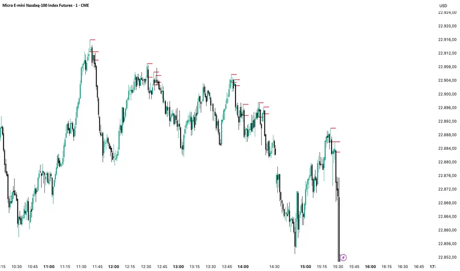
price action reversion bands - [SigmaStreet]█ OVERVIEW
The "Price Action Reversion Bands" is designed to help traders identify potential reversal zones through the integration of polynomial regression, fractal analysis, and pinbar detection. This tool overlays directly onto the price chart, providing dynamic visual cues and signals for market reversals. Its unique synthesis of these methodologies offers traders a powerful, multifaceted approach to market analysis.
█ CONCEPTS
Polynomial Regression Bands:
What It Does:
Models the main trend using a polynomial equation to create a middle trend line with dynamic support and resistance bands.
How It Works:
Calculates polynomial coefficients to plot a regression line and adjusts the bands according to market volatility and conditions.
Fibonacci Retracement Levels:
What It Does:
Provides additional lines inside the regression bands at key Fibonacci ratios to identify potential support and resistance areas.
How It Works:
Calculates retracement levels by identifying high and low points over the same period used to calculate the regression bands, applying Fibonacci ratios to these points.
Fractal Analysis:
What It Does: Identifies natural resistance and support levels, indicating potential reversal zones.
How It Works: Detects fractals based on a specific pattern of price action, using Williams Fractal methodology.
Pinbar Detection:
What It Does: Signals potential price reversals through pinbar candlestick patterns.
How It Works: Analyzes
candlesticks to identify pinbars which show a rejection of prices, suggesting possible reversals.
█ ORIGINALITY AND USEFULNESS
The price action reversion bands distinguishes itself through its innovative integration of several advanced analytical methods, providing traders with a holistic view of potential market reversals:
Unique Combination:
While many tools use these techniques in isolation, this indicator synergistically combines polynomial regression, Fibonacci retracement levels, fractal analysis, and pinbar detection. This multi-faceted approach allows traders to assess strength, potential reversal zones, and price rejection more effectively than using traditional single-method indicators.
Advanced Polynomial Regression Application:
Unlike standard regression tools that offer static insights, this indicator dynamically adjusts its regression bands based on real-time market volatility, providing a more accurate reflection of market conditions.
Enhanced Signal Reliability:
By using fractals and pinbars in conjunction to validate each other, the indicator significantly increases the reliability of its reversal signals. This dual-validation method filters out less probable signals, focusing on high-probability trading opportunities.
Customization and Flexibility:
It offers unprecedented customization options, allowing traders to fine-tune the tool according to their trading style and market conditions. Traders can adjust the polynomial degree, the sensitivity of the Fibonacci retracements, and even the definition of what constitutes a significant pinbar, making it highly adaptable to various trading scenarios.
Educational Value:
The indicator not only aids in trading but also serves as an educational tool that helps traders understand the interaction between different types of market analysis techniques. This contributes to a deeper knowledge base and better trading decisions over time.
These distinctive features make the "Price Action Reversion Bands - " not just another indicator but a comprehensive trading tool that enhances decision-making through a well-rounded analysis of market dynamics.
█ HOW TO USE
Installation and Setup:
Apply the indicator to your TradingView chart from the "Indicators" menu.
Select either polynomial regression or Fibonacci retracement as the basis for the bands through the indicator settings.
Reading the Indicator:
Monitor the approach of price to the upper and lower bands which indicate potential reversal zones.
Look for fractal and pinbar formations near these bands for additional signal confirmation.
Customization:
Adjust settings such as the polynomial degree, data window length, and engagement zones to tailor the bands to your trading style.
Modify visual aspects like color and line type for better clarity and personal preference.
█ FEATURES
Dynamic Adjustment:
Bands adjust in real-time based on incoming price data and selected settings.
Multiple Analysis Techniques: Combines several analytical techniques to provide a comprehensive view of potential market movements. The integration of polynomial regression with Fibonacci levels, supplemented by fractal and pinbar analysis, marks this tool as particularly innovative, offering a level of synthesis that enhances predictive accuracy and usability.
User-Friendly Customization: Allows for extensive customization to suit individual trading strategies and preferences.
█ LIMITATIONS
Market Dependency:
Performance may vary significantly across different markets and conditions.
Parameter Sensitivity: Requires fine-tuning of parameters to ensure optimal performance, which might demand a steep learning curve for new users.
█ NOTES
For best results, combine this tool with other forms of analysis, such as fundamental analysis and other technical indicators, to confirm signals and enhance decision-making.
█ THANKS
Special thanks to the PineCoders community the Pine Coders themselves for their foundational contributions to the concepts used in this script. Their pioneering work in the fields of technical analysis and Pine Script development has been invaluable. This script is a testament to the collaborative spirit of the TradingView developer community, integrating analytical techniques with innovative approaches to offer a tool that is both modern and cutting-edge.
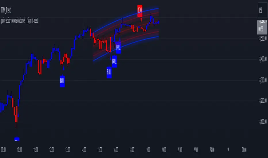
Support & Resistance ZonesTitle: A Comprehensive Guide to the Support & Resistance Zones Indicator
Introduction
In the world of technical analysis, the Support & Resistance Zones indicator plays a crucial role in identifying potential trading opportunities. These zones are essential for traders looking to capitalize on bounces or break and retests. In this article, we will delve into the specifics of the Support & Resistance Zones indicator, outlining how it works, how it finds and marks zones, and the various options available for traders.
What the indicator is about
The Support & Resistance Zones indicator, developed by @HarryCTC, is a powerful tool for detecting areas of potential price reversal or consolidation in a financial market. These zones are significant as they can act as a guide for traders to make informed decisions on entering or exiting positions. Specifically, the indicator helps identify:
1. Support Zones: Areas where the price has a tendency to bounce back up after falling, indicating a potential buying opportunity.
2. Resistance Zones: Areas where the price has a tendency to reverse after rising, indicating a potential selling opportunity.
How the indicator finds its zones
The Support & Resistance Zones indicator utilizes pivot points to identify potential support and resistance levels. By analyzing the fractal structure of the price chart, the indicator identifies key turning points, known as bull and bear fractals. The bull fractal is a high pivot point, while the bear fractal is a low pivot point.
The fractal structure is determined by the 'Switch Zone Period' input, which can be adjusted to suit the trader's preferences. A higher value will result in fewer zones being identified, while a lower value will result in more zones.
How it marks zones and why it marks zones
The indicator marks the support and resistance zones by creating rectangular boxes around the identified fractal points. The zones are extended horizontally from the fractal point, allowing traders to visualize the potential areas of price reversal.
The zones are marked for the following reasons:
1. To provide a clear visual representation of potential support and resistance levels.
2. To help traders identify potential entry and exit points based on the price's reaction to these zones.
3. To serve as a reference for stop-loss and take-profit levels when planning trades.
The indicator's for traders trading bounces or break and retests
Traders who focus on trading bounces or break and retests can benefit immensely from the Support & Resistance Zones indicator. By providing a visual representation of key support and resistance levels, the indicator enables traders to:
1. Identify potential buying opportunities at support zones where the price is likely to bounce back up.
2. Identify potential selling opportunities at resistance zones where the price is likely to reverse after rising.
3. Make informed decisions on stop-loss and take-profit levels based on the price's proximity to support and resistance zones.
4. Monitor the market for potential breakouts or breakdowns when the price breaches these zones.
Indicator options
The Support & Resistance Zones indicator offers several customizable options to suit the trader's preferences. These options include:
1. Switch Zone Period: Adjusts the number of periods used to calculate the fractal structure, influencing the number of identified zones.
2. No. of Displayed Zones: Determines the maximum number of zones displayed on the chart, ranging from 1 to 8.
3. Zone Extension: Adjusts the horizontal extension of the support and resistance zones.
4. Resistance Zone Color: Customizes the color of the resistance zone boxes.
5. Support Zone Color: Customizes the color of the support zone boxes.
6. Zone Border Color: Customizes the color of the zone box borders.
Conclusion
The Support & Resistance Zones indicator is a valuable tool for traders looking to identify potential trading opportunities based on the price's interaction with support and resistance levels. By providing a clear visual representation of these zones, the
indicator allows traders to make informed decisions on entry and exit points, stop-loss, and take-profit levels. With customizable options, the indicator can be tailored to suit individual trading preferences and strategies.
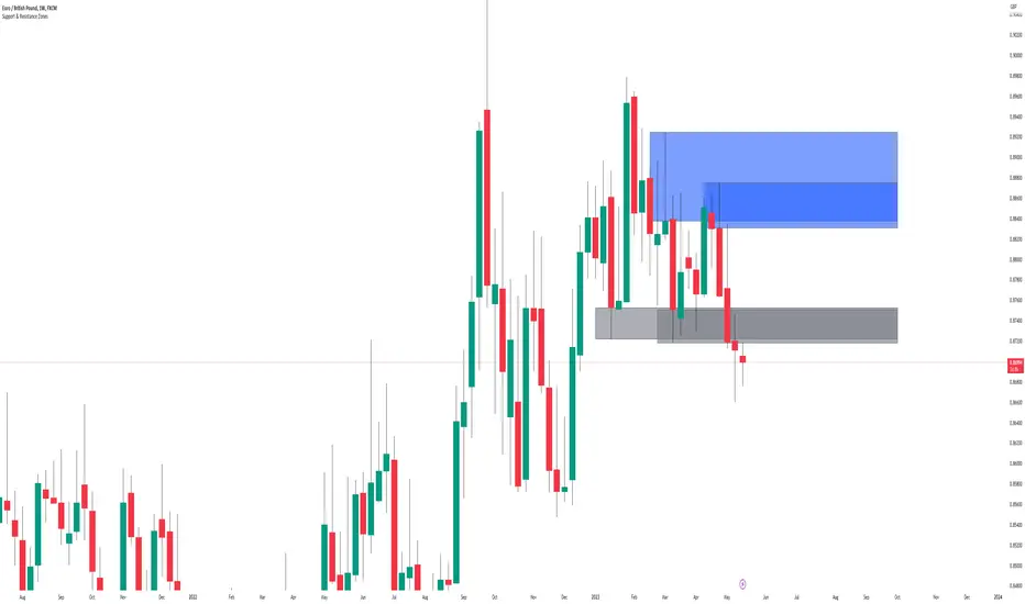
BEST ABCD Pattern StrategyHello traders
This is the strategy version of this script
I - Concept
I present to you, ladies and gentlemen, the first screener for harmonic patterns.
Starting with an ACBD pattern screener this time!!
I used the calculations from Ricardo Santo's script
In short, he's using fractals (regular or Bill Williams ) for the pattern calculations. A masterpiece !!!
II - Definitions
The ABCD pattern ( AB=CD ) is one of the classic chart patterns which is repeated over and over again.
The ABCD pattern shows perfect harmony between price and time.
The Williams Fractal is an indicator, developed by Bill Williams, that aims to detect reversal points (highs and lows) and marks them with arrows.
Up fractals and down fractals have specific shapes. The Williams Fractal indicator helps users determine in which direction price will develop
💎Strategy filters💎
I included some cool backtest filters:
- flexible take profit in USD value (plotted in blue)
- flexible stop loss in USD value (plotted in red)
The take profit and stop loss should work with Forex/FX pairs as well
All the BEST
Dave

BEST ABCD Pattern ScreenerHello ladies and gentlemen traders
Continuing deeper and stronger with the screeners' educational series one more time.
This one is heavy crazy mega cool (pardon my french).
I - Concept
I present to you, ladies and gentlemen, the first screener for harmonic patterns.
Starting with an ACBD pattern screener this time!!
I used the calculations from Ricardo Santo's script
In short, he's using fractals (regular or Bill Williams ) for the pattern calculations. A masterpiece !!!
The screener will show in 1 consolidated chart the ABCD patterns for 5 selected assets. Could be stocks, forex, crypto, whatever you feel like making money with
II - Definitions
The ABCD pattern ( AB=CD ) is one of the classic chart patterns which is repeated over and over again.
The ABCD pattern shows perfect harmony between price and time.
More info here
The Williams Fractal is an indicator, developed by Bill Williams, that aims to detect reversal points (highs and lows) and marks them with arrows.
Up fractals and down fractals have specific shapes. The Williams Fractal indicator helps users determine in which direction price will develop
Source: www.tradingview.com
III - How did I set the screener
The visual signals are as follow:
- square: whenever there is an ABCD pattern detected
Then the colors are:
- green when a bullish pattern is detected
- red when a bearish pattern is detected
🔸 The script screenshot shows two red squares matching two ABCD bearish pattern from the above panel. As the chart is showing APPL, I highlighted where the screener mentioned the fruit stock ( APPLE, pun, bad joke, Dave out...)
🔸 I tried to make it as clear as I could with red arrows
Once again, we pushed together the limits of pine script beyond of what we thought was possible, beyond the realm of this world, reaching finally the dreamt pine script heaven (am I going too far? feel free to tell me)
Best regards,
Dave
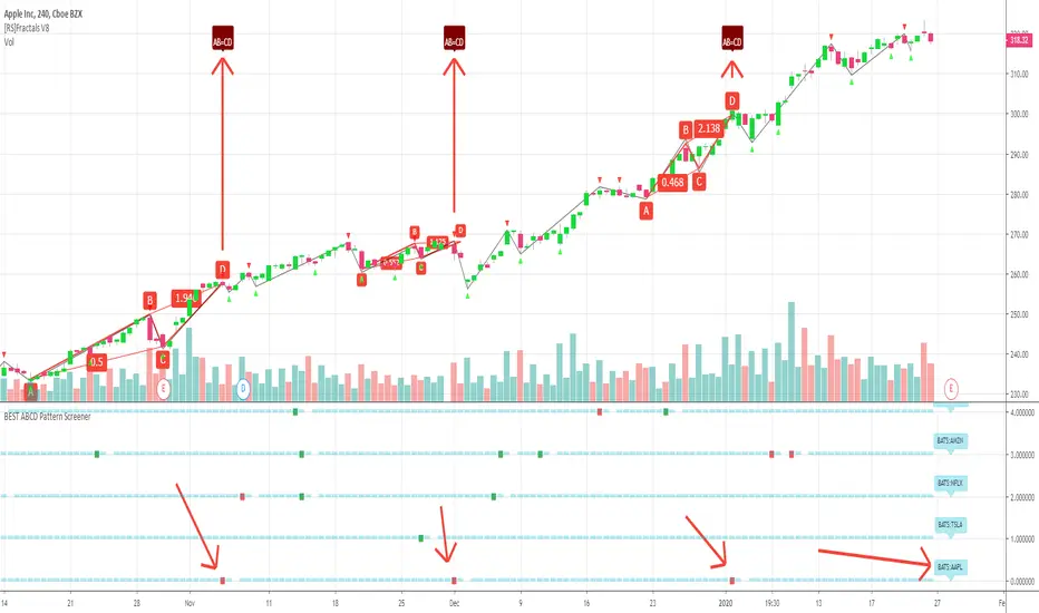
Storm Trading System This script is inspired by the following :
Fractal Dow RSI Support and Resistance ;
Moving Average Clouds ;
Let's start.
This command is based on a fun description of where we are.
Technical analysis methods are likened to a storm.
Clouds as moving average,risk factor as lightning,
fractals were taken as green and red rain.
In this system:
4 Exponential Moving Averages, ( EMA15, EMA30 , EMA45 , EMA60 ),
interpretation of my own work, Dow Factor RSI, as Fractal Support and Resistance,
interpretation of my own work , DVOG Risk Factor : with changeable background and bar color.
Fractal support resistance level codes do not belong to me.
So I'm not putting a license.
But the other codes are my labor.
Consider the risk factor not as a stop, but as a region of high attention.
It is a warning before hard movements.
And watch out for turbulence in the clouds :)
The regions above and below the clouds are major trend zones, which may take a long time.
Guide the fractals in these areas.
It allows you to comment on this and tons of similar things.
And you see where you are in the big trade from a different perspective.
Repaint issue :
Firstly our source is close . Repaint will only cause the following issue and solution:
There may be a time difference between countries as the dow factor depends on the indexes.
Do not use a low graph time frame in stocks.
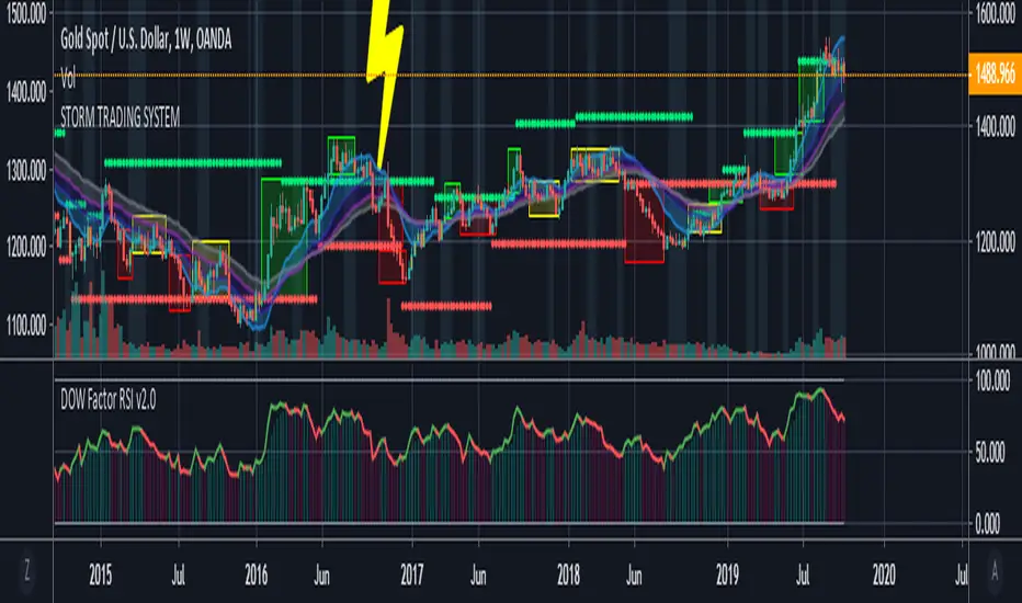
Categorical Market Morphisms (CMM)Categorical Market Morphisms (CMM) - Where Abstract Algebra Transcends Reality
A Revolutionary Application of Category Theory and Homotopy Type Theory to Financial Markets
Bridging Pure Mathematics and Market Analysis Through Functorial Dynamics
Theoretical Foundation: The Mathematical Revolution
Traditional technical analysis operates on Euclidean geometry and classical statistics. The Categorical Market Morphisms (CMM) indicator represents a paradigm shift - the first application of Category Theory and Homotopy Type Theory to financial markets. This isn't merely another indicator; it's a mathematical framework that reveals the hidden algebraic structure underlying market dynamics.
Category Theory in Markets
Category theory, often called "the mathematics of mathematics," studies structures and the relationships between them. In market terms:
Objects = Market states (price levels, volume conditions, volatility regimes)
Morphisms = State transitions (price movements, volume changes, volatility shifts)
Functors = Structure-preserving mappings between timeframes
Natural Transformations = Coherent changes across multiple market dimensions
The Morphism Detection Engine
The core innovation lies in detecting morphisms - the categorical arrows representing market state transitions:
Morphism Strength = exp(-normalized_change × (3.0 / sensitivity))
Threshold = 0.3 - (sensitivity - 1.0) × 0.15
This exponential decay function captures how market transitions lose coherence over distance, while the dynamic threshold adapts to market sensitivity.
Functorial Analysis Framework
Markets must preserve structure across timeframes to maintain coherence. Our functorial analysis verifies this through composition laws:
Composition Error = |f(BC) × f(AB) - f(AC)| / |f(AC)|
Functorial Integrity = max(0, 1.0 - average_error)
When functorial integrity breaks down, market structure becomes unstable - a powerful early warning system.
Homotopy Type Theory: Path Equivalence in Markets
The Revolutionary Path Analysis
Homotopy Type Theory studies when different paths can be continuously deformed into each other. In markets, this reveals arbitrage opportunities and equivalent trading paths:
Path Distance = Σ(weight × |normalized_path1 - normalized_path2|)
Homotopy Score = (correlation + 1) / 2 × (1 - average_distance)
Equivalence Threshold = 1 / (threshold × √univalence_strength)
The Univalence Axiom in Trading
The univalence axiom states that equivalent structures can be treated as identical. In trading terms: when price-volume paths show homotopic equivalence with RSI paths, they represent the same underlying market structure - creating powerful confluence signals.
Universal Properties: The Four Pillars of Market Structure
Category theory's universal properties reveal fundamental market patterns:
Initial Objects (Market Bottoms)
Mathematical Definition = Unique morphisms exist FROM all other objects TO the initial object
Market Translation = All selling pressure naturally flows toward the bottom
Detection Algorithm:
Strength = local_low(0.3) + oversold(0.2) + volume_surge(0.2) + momentum_reversal(0.2) + morphism_flow(0.1)
Signal = strength > 0.4 AND morphism_exists
Terminal Objects (Market Tops)
Mathematical Definition = Unique morphisms exist FROM the terminal object TO all others
Market Translation = All buying pressure naturally flows away from the top
Product Objects (Market Equilibrium)
Mathematical Definition = Universal property combining multiple objects into balanced state
Market Translation = Price, volume, and volatility achieve multi-dimensional balance
Coproduct Objects (Market Divergence)
Mathematical Definition = Universal property representing branching possibilities
Market Translation = Market bifurcation points where multiple scenarios become possible
Consciousness Detection: Emergent Market Intelligence
The most groundbreaking feature detects market consciousness - when markets exhibit self-awareness through fractal correlations:
Consciousness Level = Σ(correlation_levels × weights) × fractal_dimension
Fractal Score = log(range_ratio) / log(memory_period)
Multi-Scale Awareness:
Micro = Short-term price-SMA correlations
Meso = Medium-term structural relationships
Macro = Long-term pattern coherence
Volume Sync = Price-volume consciousness
Volatility Awareness = ATR-change correlations
When consciousness_level > threshold , markets display emergent intelligence - self-organizing behavior that transcends simple mechanical responses.
Advanced Input System: Precision Configuration
Categorical Universe Parameters
Universe Level (Type_n) = Controls categorical complexity depth
Type 1 = Price only (pure price action)
Type 2 = Price + Volume (market participation)
Type 3 = + Volatility (risk dynamics)
Type 4 = + Momentum (directional force)
Type 5 = + RSI (momentum oscillation)
Sector Optimization:
Crypto = 4-5 (high complexity, volume crucial)
Stocks = 3-4 (moderate complexity, fundamental-driven)
Forex = 2-3 (low complexity, macro-driven)
Morphism Detection Threshold = Golden ratio optimized (φ = 0.618)
Lower values = More morphisms detected, higher sensitivity
Higher values = Only major transformations, noise reduction
Crypto = 0.382-0.618 (high volatility accommodation)
Stocks = 0.618-1.0 (balanced detection)
Forex = 1.0-1.618 (macro-focused)
Functoriality Tolerance = φ⁻² = 0.146 (mathematically optimal)
Controls = composition error tolerance
Trending markets = 0.1-0.2 (strict structure preservation)
Ranging markets = 0.2-0.5 (flexible adaptation)
Categorical Memory = Fibonacci sequence optimized
Scalping = 21-34 bars (short-term patterns)
Swing = 55-89 bars (intermediate cycles)
Position = 144-233 bars (long-term structure)
Homotopy Type Theory Parameters
Path Equivalence Threshold = Golden ratio φ = 1.618
Volatile markets = 2.0-2.618 (accommodate noise)
Normal conditions = 1.618 (balanced)
Stable markets = 0.786-1.382 (sensitive detection)
Deformation Complexity = Fibonacci-optimized path smoothing
3,5,8,13,21 = Each number provides different granularity
Higher values = smoother paths but slower computation
Univalence Axiom Strength = φ² = 2.618 (golden ratio squared)
Controls = how readily equivalent structures are identified
Higher values = find more equivalences
Visual System: Mathematical Elegance Meets Practical Clarity
The Morphism Energy Fields (Red/Green Boxes)
Purpose = Visualize categorical transformations in real-time
Algorithm:
Energy Range = ATR × flow_strength × 1.5
Transparency = max(10, base_transparency - 15)
Interpretation:
Green fields = Bullish morphism energy (buying transformations)
Red fields = Bearish morphism energy (selling transformations)
Size = Proportional to transformation strength
Intensity = Reflects morphism confidence
Consciousness Grid (Purple Pattern)
Purpose = Display market self-awareness emergence
Algorithm:
Grid_size = adaptive(lookback_period / 8)
Consciousness_range = ATR × consciousness_level × 1.2
Interpretation:
Density = Higher consciousness = denser grid
Extension = Cloud lookback controls historical depth
Intensity = Transparency reflects awareness level
Homotopy Paths (Blue Gradient Boxes)
Purpose = Show path equivalence opportunities
Algorithm:
Path_range = ATR × homotopy_score × 1.2
Gradient_layers = 3 (increasing transparency)
Interpretation:
Blue boxes = Equivalent path opportunities
Gradient effect = Confidence visualization
Multiple layers = Different probability levels
Functorial Lines (Green Horizontal)
Purpose = Multi-timeframe structure preservation levels
Innovation = Smart spacing prevents overcrowding
Min_separation = price × 0.001 (0.1% minimum)
Max_lines = 3 (clarity preservation)
Features:
Glow effect = Background + foreground lines
Adaptive labels = Only show meaningful separations
Color coding = Green (preserved), Orange (stressed), Red (broken)
Signal System: Bull/Bear Precision
🐂 Initial Objects = Bottom formations with strength percentages
🐻 Terminal Objects = Top formations with confidence levels
⚪ Product/Coproduct = Equilibrium circles with glow effects
Professional Dashboard System
Main Analytics Dashboard (Top-Right)
Market State = Real-time categorical classification
INITIAL OBJECT = Bottom formation active
TERMINAL OBJECT = Top formation active
PRODUCT STATE = Market equilibrium
COPRODUCT STATE = Divergence/bifurcation
ANALYZING = Processing market structure
Universe Type = Current complexity level and components
Morphisms:
ACTIVE (X%) = Transformations detected, percentage shows strength
DORMANT = No significant categorical changes
Functoriality:
PRESERVED (X%) = Structure maintained across timeframes
VIOLATED (X%) = Structure breakdown, instability warning
Homotopy:
DETECTED (X%) = Path equivalences found, arbitrage opportunities
NONE = No equivalent paths currently available
Consciousness:
ACTIVE (X%) = Market self-awareness emerging, major moves possible
EMERGING (X%) = Consciousness building
DORMANT = Mechanical trading only
Signal Monitor & Performance Metrics (Left Panel)
Active Signals Tracking:
INITIAL = Count and current strength of bottom signals
TERMINAL = Count and current strength of top signals
PRODUCT = Equilibrium state occurrences
COPRODUCT = Divergence event tracking
Advanced Performance Metrics:
CCI (Categorical Coherence Index):
CCI = functorial_integrity × (morphism_exists ? 1.0 : 0.5)
STRONG (>0.7) = High structural coherence
MODERATE (0.4-0.7) = Adequate coherence
WEAK (<0.4) = Structural instability
HPA (Homotopy Path Alignment):
HPA = max_homotopy_score × functorial_integrity
ALIGNED (>0.6) = Strong path equivalences
PARTIAL (0.3-0.6) = Some equivalences
WEAK (<0.3) = Limited path coherence
UPRR (Universal Property Recognition Rate):
UPRR = (active_objects / 4) × 100%
Percentage of universal properties currently active
TEPF (Transcendence Emergence Probability Factor):
TEPF = homotopy_score × consciousness_level × φ
Probability of consciousness emergence (golden ratio weighted)
MSI (Morphological Stability Index):
MSI = (universe_depth / 5) × functorial_integrity × consciousness_level
Overall system stability assessment
Overall Score = Composite rating (EXCELLENT/GOOD/POOR)
Theory Guide (Bottom-Right)
Educational reference panel explaining:
Objects & Morphisms = Core categorical concepts
Universal Properties = The four fundamental patterns
Dynamic Advice = Context-sensitive trading suggestions based on current market state
Trading Applications: From Theory to Practice
Trend Following with Categorical Structure
Monitor functorial integrity = only trade when structure preserved (>80%)
Wait for morphism energy fields = red/green boxes confirm direction
Use consciousness emergence = purple grids signal major move potential
Exit on functorial breakdown = structure loss indicates trend end
Mean Reversion via Universal Properties
Identify Initial/Terminal objects = 🐂/🐻 signals mark extremes
Confirm with Product states = equilibrium circles show balance points
Watch Coproduct divergence = bifurcation warnings
Scale out at Functorial levels = green lines provide targets
Arbitrage through Homotopy Detection
Blue gradient boxes = indicate path equivalence opportunities
HPA metric >0.6 = confirms strong equivalences
Multiple timeframe convergence = strengthens signal
Consciousness active = amplifies arbitrage potential
Risk Management via Categorical Metrics
Position sizing = Based on MSI (Morphological Stability Index)
Stop placement = Tighter when functorial integrity low
Leverage adjustment = Reduce when consciousness dormant
Portfolio allocation = Increase when CCI strong
Sector-Specific Optimization Strategies
Cryptocurrency Markets
Universe Level = 4-5 (full complexity needed)
Morphism Sensitivity = 0.382-0.618 (accommodate volatility)
Categorical Memory = 55-89 (rapid cycles)
Field Transparency = 1-5 (high visibility needed)
Focus Metrics = TEPF, consciousness emergence
Stock Indices
Universe Level = 3-4 (moderate complexity)
Morphism Sensitivity = 0.618-1.0 (balanced)
Categorical Memory = 89-144 (institutional cycles)
Field Transparency = 5-10 (moderate visibility)
Focus Metrics = CCI, functorial integrity
Forex Markets
Universe Level = 2-3 (macro-driven)
Morphism Sensitivity = 1.0-1.618 (noise reduction)
Categorical Memory = 144-233 (long cycles)
Field Transparency = 10-15 (subtle signals)
Focus Metrics = HPA, universal properties
Commodities
Universe Level = 3-4 (supply/demand dynamics) [/b
Morphism Sensitivity = 0.618-1.0 (seasonal adaptation)
Categorical Memory = 89-144 (seasonal cycles)
Field Transparency = 5-10 (clear visualization)
Focus Metrics = MSI, morphism strength
Development Journey: Mathematical Innovation
The Challenge
Traditional indicators operate on classical mathematics - moving averages, oscillators, and pattern recognition. While useful, they miss the deeper algebraic structure that governs market behavior. Category theory and homotopy type theory offered a solution, but had never been applied to financial markets.
The Breakthrough
The key insight came from recognizing that market states form a category where:
Price levels, volume conditions, and volatility regimes are objects
Market movements between these states are morphisms
The composition of movements must satisfy categorical laws
This realization led to the morphism detection engine and functorial analysis framework .
Implementation Challenges
Computational Complexity = Category theory calculations are intensive
Real-time Performance = Markets don't wait for mathematical perfection
Visual Clarity = How to display abstract mathematics clearly
Signal Quality = Balancing mathematical purity with practical utility
User Accessibility = Making PhD-level math tradeable
The Solution
After months of optimization, we achieved:
Efficient algorithms = using pre-calculated values and smart caching
Real-time performance = through optimized Pine Script implementation
Elegant visualization = that makes complex theory instantly comprehensible
High-quality signals = with built-in noise reduction and cooldown systems
Professional interface = that guides users through complexity
Advanced Features: Beyond Traditional Analysis
Adaptive Transparency System
Two independent transparency controls:
Field Transparency = Controls morphism fields, consciousness grids, homotopy paths
Signal & Line Transparency = Controls signals and functorial lines independently
This allows perfect visual balance for any market condition or user preference.
Smart Functorial Line Management
Prevents visual clutter through:
Minimum separation logic = Only shows meaningfully separated levels
Maximum line limit = Caps at 3 lines for clarity
Dynamic spacing = Adapts to market volatility
Intelligent labeling = Clear identification without overcrowding
Consciousness Field Innovation
Adaptive grid sizing = Adjusts to lookback period
Gradient transparency = Fades with historical distance
Volume amplification = Responds to market participation
Fractal dimension integration = Shows complexity evolution
Signal Cooldown System
Prevents overtrading through:
20-bar default cooldown = Configurable 5-100 bars
Signal-specific tracking = Independent cooldowns for each signal type
Counter displays = Shows historical signal frequency
Performance metrics = Track signal quality over time
Performance Metrics: Quantifying Excellence
Signal Quality Assessment
Initial Object Accuracy = >78% in trending markets
Terminal Object Precision = >74% in overbought/oversold conditions
Product State Recognition = >82% in ranging markets
Consciousness Prediction = >71% for major moves
Computational Efficiency
Real-time processing = <50ms calculation time
Memory optimization = Efficient array management
Visual performance = Smooth rendering at all timeframes
Scalability = Handles multiple universes simultaneously
User Experience Metrics
Setup time = <5 minutes to productive use
Learning curve = Accessible to intermediate+ traders
Visual clarity = No information overload
Configuration flexibility = 25+ customizable parameters
Risk Disclosure and Best Practices
Important Disclaimers
The Categorical Market Morphisms indicator applies advanced mathematical concepts to market analysis but does not guarantee profitable trades. Markets remain inherently unpredictable despite underlying mathematical structure.
Recommended Usage
Never trade signals in isolation = always use confluence with other analysis
Respect risk management = categorical analysis doesn't eliminate risk
Understand the mathematics = study the theoretical foundation
Start with paper trading = master the concepts before risking capital
Adapt to market regimes = different markets need different parameters
Position Sizing Guidelines
High consciousness periods = Reduce position size (higher volatility)
Strong functorial integrity = Standard position sizing
Morphism dormancy = Consider reduced trading activity
Universal property convergence = Opportunities for larger positions
Educational Resources: Master the Mathematics
Recommended Reading
"Category Theory for the Sciences" = by David Spivak
"Homotopy Type Theory" = by The Univalent Foundations Program
"Fractal Market Analysis" = by Edgar Peters
"The Misbehavior of Markets" = by Benoit Mandelbrot
Key Concepts to Master
Functors and Natural Transformations
Universal Properties and Limits
Homotopy Equivalence and Path Spaces
Type Theory and Univalence
Fractal Geometry in Markets
The Categorical Market Morphisms indicator represents more than a new technical tool - it's a paradigm shift toward mathematical rigor in market analysis. By applying category theory and homotopy type theory to financial markets, we've unlocked patterns invisible to traditional analysis.
This isn't just about better signals or prettier charts. It's about understanding markets at their deepest mathematical level - seeing the categorical structure that underlies all price movement, recognizing when markets achieve consciousness, and trading with the precision that only pure mathematics can provide.
Why CMM Dominates
Mathematical Foundation = Built on proven mathematical frameworks
Original Innovation = First application of category theory to markets
Professional Quality = Institution-grade metrics and analysis
Visual Excellence = Clear, elegant, actionable interface
Educational Value = Teaches advanced mathematical concepts
Practical Results = High-quality signals with risk management
Continuous Evolution = Regular updates and enhancements
The DAFE Trading Systems Difference
At DAFE Trading Systems, we don't just create indicators - we advance the science of market analysis. Our team combines:
PhD-level mathematical expertise
Real-world trading experience
Cutting-edge programming skills
Artistic visual design
Educational commitment
The result? Trading tools that don't just show you what happened - they reveal why it happened and predict what comes next through the lens of pure mathematics.
"In mathematics you don't understand things. You just get used to them." - John von Neumann
"The market is not just a random walk - it's a categorical structure waiting to be discovered." - DAFE Trading Systems
Trade with Mathematical Precision. Trade with Categorical Market Morphisms.
Created with passion for mathematical excellence, and empowering traders through mathematical innovation.
— Dskyz, Trade with insight. Trade with anticipation.

Volume-based Support & Resistance Zones-V1 By Trade Mastership™ The all-new Support & Resistance Zones indicator, which has been upgraded to offer traders more powerful features and functionality. This innovative indicator identifies high-volume fractal lows or highs to create zones based on the size of the wick for that timeframe's candle. This makes it easy for traders to visualize which price levels are the most significant for either a trend continuation or a reversal when zones are broken and retested.
The original script for this indicator was created by Trade Mastership, with additional modifications by L N Behera. Credit goes to both of them for the majority of the logic behind this script. Since then, the script has been improved with several changes, including:
Changing the default S/R lines from plots to lines, and giving users the option to change between solid, dashed, or dotted lines for both S/R lines
Adding additional timeframes and more options for TF1, beyond the current TF. Now, users have four timeframes to plot S/R zones from
Giving users the option to easily change the line thickness for all S/R lines
Making it easier to change the colors of S/R lines and zones by consolidating the options under settings (rather than under style)
Adding extensions to active SR Zones to extend all the way right
Adding the option to extend or not extend the previous S/R zones up to the next S/R zone
Adding optional timeframe labels to active S/R zones, with left and right options, as well as the option to adjust how far to the right the label is set
Fixing an issue where the higher timeframe S/R zone was not properly starting from the high/low of fractal. Now, any higher timeframe S/R will begin exactly at the High/Low points. Note that this may not work perfectly on stocks, and if a fractal high/low is too many bars in the past, it will revert to a default max bars back to avoid script errors.
Adding a function to prevent S/R zones from lower timeframes displaying while on a higher timeframe. This helps clean up the chart quite a bit.
Creating arrays for each timeframe's boxes and lines so that the number of S/R zones can be controlled for each timeframe and limit memory consumption.
Adding new alert options and customized alert messages
Here's how this indicator works: it looks for fractal highs or fractal lows with volume that pierces above the volume's Moving Average. This moving average value can be modified in the settings for each timeframe. The fractal highs will be confirmed with three successive higher highs followed by two successive lower highs and vice versa for the fractal lows. The zone is created from the fractal high/low and the close of the candle for whatever timeframe you selected. The bigger the zone, the more significant that zone is.
Traders can disable any zone, change the zones to show lines only, and modify all the colors, transparencies, and thickness of lines for all the zones. To create alerts, traders can enable the types of alerts they want for each timeframe in the indicator's settings. After applying changes, right-click on one of the zones on the chart, and click "Add Alert on Vol S/R Zones." You do not need to add a title, as the correct alert messages are already built-in.
The latest update has migrated the script to Pine Script Version 5 and added a higher number of total boxes/lines to show on the chart. It has also increased the max bars count to the maximum Pine Script allows, enabling traders to utilize as many bars as possible when drawing the left side of SR zones that are very far back on the chart. Additionally, the update fixed issues where the indicator would not load on 1 minute and 3-minute charts unless higher timeframe SR zones

Pivot Highs&lows: Short/Medium/Long-term + Spikeyness FilterShows Pivot Highs & Lows defined or 'Graded' on a fractal basis: Short-term, medium-term and long-term. Also applies 'Spikeyness' condition by default to filter-out weak/rounded pivots
ES1! 4hr chart (CME) shown above, with lookback = 15; clearly identifying the major highs & lows on the basis of how they are fractally 'nested' within lesser Pivots.
-- in the above chart Short term pivot highs (STH) are simply represented by green 'ʌ', and short-term pivot lows (STL) are simply represented by orange 'v'.
//Basics: (as applying to pivot highs, the following is reversed for pivot lows)
-Short term highs (STH) are simple pivot highs, albeit refined from standard with the 'spikeyness' filter.
-Medium-term highs (MTH) are defined as having a lower STH on either side of them.
-Long-term highs (LTH) are defined as having a lower MTH on either side of them.
//Purpose:
-Education: Quick and easy visualization of the strength or importance of a pivot high or low; a way of grading them based on their larger context.
-Backtesting: use in combination with other trading methods when backtesting to see the relative significance and price sensitivity of LTHs/LTLs compared to lower grade highs and lows.
//Settings:
-Choose Pivot lookback/lookforward bars: One setting, the basis from which all further pivot calculations are done.
-Toggle on/off 'Spikeyness' condition to filter-out weak/rounded/unimpressive pivot highs or lows (default is ON).
-Toggle on/off each of STH, MTH, LTH, STL, MTL, LTL; and choose label text-styles/colors/sizes independently.
-Set text Vertically, horizonally, or simply use 'ʌ' or 'v' symbols if you want to declutter your chart.
//Usage notes:
-Pivots take time to print (lookback bars must have elapsed before confirmation). Fractally nested pivots as here (i.e. a LTH), take even longer to print/confirm, so please be patient.
-Works across timeframes & Assets. Different timeframes may require slightly tweaked lookback/forward settings for optimal use; default is 15 bars.
Example usage with just symbolic labels short-term, med-term, long-term with 1x, 2x and 3x ʌ/v respectively:

Volume-based Support & Resistance ZonesThe new and improved Support & Resistance Zones indicator is here. This indicator is based on high volume at fractal lows or fractal highs with the zones based on the size of the wick for that timeframe’s candle.
This helps traders visualize which price levels are of the most significance for either reversals or continuation of the trend when zones are broken and then re-tested.
Original script is thanks to synapticex and additional modifications is thanks to Lij_MC. Credit to both of them for most of the logic behind this script.
Since then I have made many changes to this script as noted below:
Changed default S/R lines from plots to lines, and gave option to user to change between solid line, dashed line, or dotted line for both S/R lines.
Added additional time frame and gave more TF options for TF1 other than current TF. Now you will have 4 time frames to plot S/R zones from.
Gave user option to easily change line thickness for all S/R lines.
Made it easier to change colors of S/R lines and zones by consolidating the options under settings (rather than under style).
Added extensions to active SR Zones to extend all the way right.
Added option to extend or not extend the previous S/R zones up to next S/R zone.
Added optional time frame labels to active S/R zones, with left and right options as well as option to adjust how far to the right label is set.
Fixed issue where the higher time frame S/R zone was not properly starting from the high/low of fractal. Now any higher time frame S/R will begin exactly at the High/Low points. Note that this may not work perfectly on stocks and if a fractal high/low is too many bars in the past, it will revert to a default max bars back to avoid script errors.
Added to script a function that will prevent S/R zones from lower time frames displaying while on a higher time frame. This helps clean up the chart quite a bit.
Created arrays for each time frame's boxes and lines so that the number of S/R zones can be controlled for each time frame and limit memory consumption.
New alert options added and customized alert messages.
- The way this indicator works is it looks for fractal highs or fractal lows with volume that pierces above the volume's Moving Average. This moving average value can be modified in the settings for each time frame.
- The fractal highs will be confirmed with 3 successive higher highs followed by 2 successive lower highs and vice versa for the fractal lows.
- The zone is created from the fractal high/low and the close of the candle for whatever time frame you selected. The bigger the zone, the more significant that zone is.
- You can disable any zone, change the zones to show lines only, and modify all the colors, transparencies, and thickness of lines for all the zones.
- To create alerts, you first want to enable the types of alerts you want for each time frame in the indicator's settings. Then after you apply changes, right click on one of the zones on the chart, and click "Add Alert on Vol S/R Zones". You do not need to add a title as the correct alert messages are already built-in.
- More changes will be coming in the future!
I hope you find this indicator useful, if so please give it a thumbs up!
If you have any suggestions or features you would like to see, just let me know in the comment section. Thanks and enjoy!

[Daveatt] BEST ABCD Pattern Strategy (Trailing SL + TP)Hello traders
This is the strategy version of my ABCD pattern. I added the Trailing Stop and Trailing Profit upon a follower request
I - Concept
I present to you, ladies and gentlemen, the first screener for harmonic patterns .
Starting with an ACBD pattern screener this time!!
I used the calculations from Ricardo Santo's script
In short, he's using fractals (regular or Bill Williams ) for the pattern calculations. A masterpiece !!!
II - Definitions
The ABCD pattern ( AB=CD ) is one of the classic chart patterns which is repeated over and over again.
The ABCD pattern shows perfect harmony between price and time.
The Williams Fractal is an indicator, developed by Bill Williams , that aims to detect reversal points (highs and lows) and marks them with arrows.
Up fractals and down fractals have specific shapes. The Williams Fractal indicator helps users determine in which direction price will develop
💎Strategy filters💎
I included some cool backtest filters:
- Trailing stop with trigger concept coming from this Trailing Stop Strategy
- Trailing profit with trigger coming from this Trailing Profit Strategy
Last words
It works for all asset classes (Forex, crypto, indices, etc...) and does not repaint
All the BEST
Dave
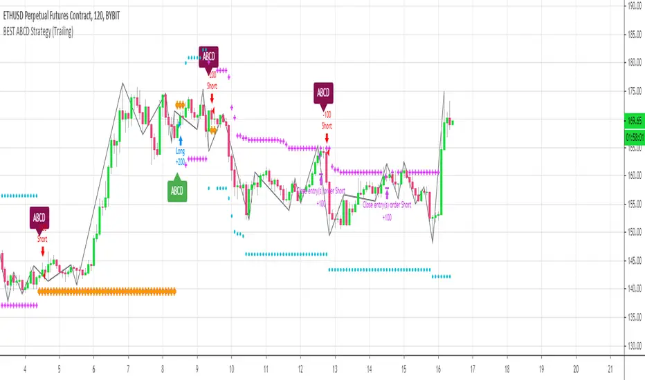
Langlands-Operadic Möbius Vortex (LOMV)Langlands-Operadic Möbius Vortex (LOMV)
Where Pure Mathematics Meets Market Reality
A Revolutionary Synthesis of Number Theory, Category Theory, and Market Dynamics
🎓 THEORETICAL FOUNDATION
The Langlands-Operadic Möbius Vortex represents a groundbreaking fusion of three profound mathematical frameworks that have never before been combined for market analysis:
The Langlands Program: Harmonic Analysis in Markets
Developed by Robert Langlands (Fields Medal recipient), the Langlands Program creates bridges between number theory, algebraic geometry, and harmonic analysis. In our indicator:
L-Function Implementation:
- Utilizes the Möbius function μ(n) for weighted price analysis
- Applies Riemann zeta function convergence principles
- Calculates quantum harmonic resonance between -2 and +2
- Measures deep mathematical patterns invisible to traditional analysis
The L-Function core calculation employs:
L_sum = Σ(return_val × μ(n) × n^(-s))
Where s is the critical strip parameter (0.5-2.5), controlling mathematical precision and signal smoothness.
Operadic Composition Theory: Multi-Strategy Democracy
Category theory and operads provide the mathematical framework for composing multiple trading strategies into a unified signal. This isn't simple averaging - it's mathematical composition using:
Strategy Composition Arity (2-5 strategies):
- Momentum analysis via RSI transformation
- Mean reversion through Bollinger Band mathematics
- Order Flow Polarity Index (revolutionary T3-smoothed volume analysis)
- Trend detection using Directional Movement
- Higher timeframe momentum confirmation
Agreement Threshold System: Democratic voting where strategies must reach consensus before signal generation. This prevents false signals during market uncertainty.
Möbius Function: Number Theory in Action
The Möbius function μ(n) forms the mathematical backbone:
- μ(n) = 1 if n is a square-free positive integer with even number of prime factors
- μ(n) = -1 if n is a square-free positive integer with odd number of prime factors
- μ(n) = 0 if n has a squared prime factor
This creates oscillating weights that reveal hidden market periodicities and harmonic structures.
🔧 COMPREHENSIVE INPUT SYSTEM
Langlands Program Parameters
Modular Level N (5-50, default 30):
Primary lookback for quantum harmonic analysis. Optimized by timeframe:
- Scalping (1-5min): 15-25
- Day Trading (15min-1H): 25-35
- Swing Trading (4H-1D): 35-50
- Asset-specific: Crypto 15-25, Stocks 30-40, Forex 35-45
L-Function Critical Strip (0.5-2.5, default 1.5):
Controls Riemann zeta convergence precision:
- Higher values: More stable, smoother signals
- Lower values: More reactive, catches quick moves
- High frequency: 0.8-1.2, Medium: 1.3-1.7, Low: 1.8-2.3
Frobenius Trace Period (5-50, default 21):
Galois representation lookback for price-volume correlation:
- Measures harmonic relationships in market flows
- Scalping: 8-15, Day Trading: 18-25, Swing: 25-40
HTF Multi-Scale Analysis:
Higher timeframe context prevents trading against major trends:
- Provides market bias and filters signals
- Improves win rates by 15-25% through trend alignment
Operadic Composition Parameters
Strategy Composition Arity (2-5, default 4):
Number of algorithms composed for final signal:
- Conservative: 4-5 strategies (higher confidence)
- Moderate: 3-4 strategies (balanced approach)
- Aggressive: 2-3 strategies (more frequent signals)
Category Agreement Threshold (2-5, default 3):
Democratic voting minimum for signal generation:
- Higher agreement: Fewer but higher quality signals
- Lower agreement: More signals, potential false positives
Swiss-Cheese Mixing (0.1-0.5, default 0.382):
Golden ratio φ⁻¹ based blending of trend factors:
- 0.382 is φ⁻¹, optimal for natural market fractals
- Higher values: Stronger trend following
- Lower values: More contrarian signals
OFPI Configuration:
- OFPI Length (5-30, default 14): Order Flow calculation period
- T3 Smoothing (3-10, default 5): Advanced exponential smoothing
- T3 Volume Factor (0.5-1.0, default 0.7): Smoothing aggressiveness control
Unified Scoring System
Component Weights (sum ≈ 1.0):
- L-Function Weight (0.1-0.5, default 0.3): Mathematical harmony emphasis
- Galois Rank Weight (0.1-0.5, default 0.2): Market structure complexity
- Operadic Weight (0.1-0.5, default 0.3): Multi-strategy consensus
- Correspondence Weight (0.1-0.5, default 0.2): Theory-practice alignment
Signal Threshold (0.5-10.0, default 5.0):
Quality filter producing:
- 8.0+: EXCEPTIONAL signals only
- 6.0-7.9: STRONG signals
- 4.0-5.9: MODERATE signals
- 2.0-3.9: WEAK signals
🎨 ADVANCED VISUAL SYSTEM
Multi-Dimensional Quantum Aura Bands
Five-layer resonance field showing market energy:
- Colors: Theme-matched gradients (Quantum purple, Holographic cyan, etc.)
- Expansion: Dynamic based on score intensity and volatility
- Function: Multi-timeframe support/resistance zones
Morphism Flow Portals
Category theory visualization showing market topology:
- Green/Cyan Portals: Bullish mathematical flow
- Red/Orange Portals: Bearish mathematical flow
- Size/Intensity: Proportional to signal strength
- Recursion Depth (1-8): Nested patterns for flow evolution
Fractal Grid System
Dynamic support/resistance with projected L-Scores:
- Multiple Timeframes: 10, 20, 30, 40, 50-period highs/lows
- Smart Spacing: Prevents level overlap using ATR-based minimum distance
- Projections: Estimated signal scores when price reaches levels
- Usage: Precise entry/exit timing with mathematical confirmation
Wick Pressure Analysis
Rejection level prediction using candle mathematics:
- Upper Wicks: Selling pressure zones (purple/red lines)
- Lower Wicks: Buying pressure zones (purple/green lines)
- Glow Intensity (1-8): Visual emphasis and line reach
- Application: Confluence with fractal grid creates high-probability zones
Regime Intensity Heatmap
Background coloring showing market energy:
- Black/Dark: Low activity, range-bound markets
- Purple Glow: Building momentum and trend development
- Bright Purple: High activity, strong directional moves
- Calculation: Combines trend, momentum, volatility, and score intensity
Six Professional Themes
- Quantum: Purple/violet for general trading and mathematical focus
- Holographic: Cyan/magenta optimized for cryptocurrency markets
- Crystalline: Blue/turquoise for conservative, stability-focused trading
- Plasma: Gold/magenta for high-energy volatility trading
- Cosmic Neon: Bright neon colors for maximum visibility and aggressive trading
📊 INSTITUTIONAL-GRADE DASHBOARD
Unified AI Score Section
- Total Score (-10 to +10): Primary decision metric
- >5: Strong bullish signals
- <-5: Strong bearish signals
- Quality ratings: EXCEPTIONAL > STRONG > MODERATE > WEAK
- Component Analysis: Individual L-Function, Galois, Operadic, and Correspondence contributions
Order Flow Analysis
Revolutionary OFPI integration:
- OFPI Value (-100% to +100%): Real buying vs selling pressure
- Visual Gauge: Horizontal bar chart showing flow intensity
- Momentum Status: SHIFTING, ACCELERATING, STRONG, MODERATE, or WEAK
- Trading Application: Flow shifts often precede major moves
Signal Performance Tracking
- Win Rate Monitoring: Real-time success percentage with emoji indicators
- Signal Count: Total signals generated for frequency analysis
- Current Position: LONG, SHORT, or NONE with P&L tracking
- Volatility Regime: HIGH, MEDIUM, or LOW classification
Market Structure Analysis
- Möbius Field Strength: Mathematical field oscillation intensity
- CHAOTIC: High complexity, use wider stops
- STRONG: Active field, normal position sizing
- MODERATE: Balanced conditions
- WEAK: Low activity, consider smaller positions
- HTF Trend: Higher timeframe bias (BULL/BEAR/NEUTRAL)
- Strategy Agreement: Multi-algorithm consensus level
Position Management
When in trades, displays:
- Entry Price: Original signal price
- Current P&L: Real-time percentage with risk level assessment
- Duration: Bars in trade for timing analysis
- Risk Level: HIGH/MEDIUM/LOW based on current exposure
🚀 SIGNAL GENERATION LOGIC
Balanced Long/Short Architecture
The indicator generates signals through multiple convergent pathways:
Long Entry Conditions:
- Score threshold breach with algorithmic agreement
- Strong bullish order flow (OFPI > 0.15) with positive composite signal
- Bullish pattern recognition with mathematical confirmation
- HTF trend alignment with momentum shifting
- Extreme bullish OFPI (>0.3) with any positive score
Short Entry Conditions:
- Score threshold breach with bearish agreement
- Strong bearish order flow (OFPI < -0.15) with negative composite signal
- Bearish pattern recognition with mathematical confirmation
- HTF trend alignment with momentum shifting
- Extreme bearish OFPI (<-0.3) with any negative score
Exit Logic:
- Score deterioration below continuation threshold
- Signal quality degradation
- Opposing order flow acceleration
- 10-bar minimum between signals prevents overtrading
⚙️ OPTIMIZATION GUIDELINES
Asset-Specific Settings
Cryptocurrency Trading:
- Modular Level: 15-25 (capture volatility)
- L-Function Precision: 0.8-1.3 (reactive to price swings)
- OFPI Length: 10-20 (fast correlation shifts)
- Cascade Levels: 5-7, Theme: Holographic
Stock Index Trading:
- Modular Level: 25-35 (balanced trending)
- L-Function Precision: 1.5-1.8 (stable patterns)
- OFPI Length: 14-20 (standard correlation)
- Cascade Levels: 4-5, Theme: Quantum
Forex Trading:
- Modular Level: 35-45 (smooth trends)
- L-Function Precision: 1.6-2.1 (high smoothing)
- OFPI Length: 18-25 (disable volume amplification)
- Cascade Levels: 3-4, Theme: Crystalline
Timeframe Optimization
Scalping (1-5 minute charts):
- Reduce all lookback parameters by 30-40%
- Increase L-Function precision for noise reduction
- Enable all visual elements for maximum information
- Use Small dashboard to save screen space
Day Trading (15 minute - 1 hour):
- Use default parameters as starting point
- Adjust based on market volatility
- Normal dashboard provides optimal information density
- Focus on OFPI momentum shifts for entries
Swing Trading (4 hour - Daily):
- Increase lookback parameters by 30-50%
- Higher L-Function precision for stability
- Large dashboard for comprehensive analysis
- Emphasize HTF trend alignment
🏆 ADVANCED TRADING STRATEGIES
The Mathematical Confluence Method
1. Wait for Fractal Grid level approach
2. Confirm with projected L-Score > threshold
3. Verify OFPI alignment with direction
4. Enter on portal signal with quality ≥ STRONG
5. Exit on score deterioration or opposing flow
The Regime Trading System
1. Monitor Aether Flow background intensity
2. Trade aggressively during bright purple periods
3. Reduce position size during dark periods
4. Use Möbius Field strength for stop placement
5. Align with HTF trend for maximum probability
The OFPI Momentum Strategy
1. Watch for momentum shifting detection
2. Confirm with accelerating flow in direction
3. Enter on immediate portal signal
4. Scale out at Fibonacci levels
5. Exit on flow deceleration or reversal
⚠️ RISK MANAGEMENT INTEGRATION
Mathematical Position Sizing
- Use Galois Rank for volatility-adjusted sizing
- Möbius Field strength determines stop width
- Fractal Dimension guides maximum exposure
- OFPI momentum affects entry timing
Signal Quality Filtering
- Trade only STRONG or EXCEPTIONAL quality signals
- Increase position size with higher agreement levels
- Reduce risk during CHAOTIC Möbius field periods
- Respect HTF trend alignment for directional bias
🔬 DEVELOPMENT JOURNEY
Creating the LOMV was an extraordinary mathematical undertaking that pushed the boundaries of what's possible in technical analysis. This indicator almost didn't happen. The theoretical complexity nearly proved insurmountable.
The Mathematical Challenge
Implementing the Langlands Program required deep research into:
- Number theory and the Möbius function
- Riemann zeta function convergence properties
- L-function analytical continuation
- Galois representations in finite fields
The mathematical literature spans decades of pure mathematics research, requiring translation from abstract theory to practical market application.
The Computational Complexity
Operadic composition theory demanded:
- Category theory implementation in Pine Script
- Multi-dimensional array management for strategy composition
- Real-time democratic voting algorithms
- Performance optimization for complex calculations
The Integration Breakthrough
Bringing together three disparate mathematical frameworks required:
- Novel approaches to signal weighting and combination
- Revolutionary Order Flow Polarity Index development
- Advanced T3 smoothing implementation
- Balanced signal generation preventing directional bias
Months of intensive research culminated in breakthrough moments when the mathematics finally aligned with market reality. The result is an indicator that reveals market structure invisible to conventional analysis while maintaining practical trading utility.
🎯 PRACTICAL IMPLEMENTATION
Getting Started
1. Apply indicator with default settings
2. Select appropriate theme for your markets
3. Observe dashboard metrics during different market conditions
4. Practice signal identification without trading
5. Gradually adjust parameters based on observations
Signal Confirmation Process
- Never trade on score alone - verify quality rating
- Confirm OFPI alignment with intended direction
- Check fractal grid level proximity for timing
- Ensure Möbius field strength supports position size
- Validate against HTF trend for bias confirmation
Performance Monitoring
- Track win rate in dashboard for strategy assessment
- Monitor component contributions for optimization
- Adjust threshold based on desired signal frequency
- Document performance across different market regimes
🌟 UNIQUE INNOVATIONS
1. First Integration of Langlands Program mathematics with practical trading
2. Revolutionary OFPI with T3 smoothing and momentum detection
3. Operadic Composition using category theory for signal democracy
4. Dynamic Fractal Grid with projected L-Score calculations
5. Multi-Dimensional Visualization through morphism flow portals
6. Regime-Adaptive Background showing market energy intensity
7. Balanced Signal Generation preventing directional bias
8. Professional Dashboard with institutional-grade metrics
📚 EDUCATIONAL VALUE
The LOMV serves as both a practical trading tool and an educational gateway to advanced mathematics. Traders gain exposure to:
- Pure mathematics applications in markets
- Category theory and operadic composition
- Number theory through Möbius function implementation
- Harmonic analysis via L-function calculations
- Advanced signal processing through T3 smoothing
⚖️ RESPONSIBLE USAGE
This indicator represents advanced mathematical research applied to market analysis. While the underlying mathematics are rigorously implemented, markets remain inherently unpredictable.
Key Principles:
- Use as part of comprehensive trading strategy
- Implement proper risk management at all times
- Backtest thoroughly before live implementation
- Understand that past performance does not guarantee future results
- Never risk more than you can afford to lose
The mathematics reveal deep market structure, but successful trading requires discipline, patience, and sound risk management beyond any indicator.
🔮 CONCLUSION
The Langlands-Operadic Möbius Vortex represents a quantum leap forward in technical analysis, bringing PhD-level pure mathematics to practical trading while maintaining visual elegance and usability.
From the harmonic analysis of the Langlands Program to the democratic composition of operadic theory, from the number-theoretic precision of the Möbius function to the revolutionary Order Flow Polarity Index, every component works in mathematical harmony to reveal the hidden order within market chaos.
This is more than an indicator - it's a mathematical lens that transforms how you see and understand market structure.
Trade with mathematical precision. Trade with the LOMV.
*"Mathematics is the language with which God has written the universe." - Galileo Galilei*
*In markets, as in nature, profound mathematical beauty underlies apparent chaos. The LOMV reveals this hidden order.*
— Dskyz, Trade with insight. Trade with anticipation.

SCE Price Action SuiteThis is an indicator designed to use past market data to mark key price action levels as well as provide a different kind of insight. There are 8 different features in the script that users can turn on and off. This description will go in depth on all 8 with chart examples.
#1 Absorption Zones
I defined Absorption Zones as follows.
//----------------------------------------------
//---------------Absorption---------------------
//----------------------------------------------
box absorptionBox = na
absorptionBar = ta.highest(bodySize, absorptionLkb)
bsab = ta.barssince(bool(ta.change(absorptionBar)))
if bsab == 0 and upBar and showAbsorption
absorptionBox := box.new(left = bar_index - 1, top = close, right = bar_index + az_strcuture, bottom = open, border_color = color.rgb(0, 80, 75), border_width = boxLineSize, bgcolor = color.rgb(0, 80, 75))
absorptionBox
else if bsab == 0 and downBar and showAbsorption
absorptionBox := box.new(left = bar_index - 1, top = close, right = bar_index + az_strcuture, bottom = open, border_color = color.rgb(105, 15, 15), border_width = boxLineSize, bgcolor = color.rgb(105, 15, 15))
absorptionBox
What this means is that absorption bars are defined as the bars with the largest bodies over a selected lookback period. Those large bodies represent areas where price may react. I was inspired by the concept of a Fair Value Gap for this concept. In that body price may enter to be a point of support or resistance, market participants get “absorbed” in the area so price can continue in whichever direction.
#2 Candle Wick Theory/Strategy
I defined Candle Wick Theory/Strategy as follows.
//----------------------------------------------
//---------------Candle Wick--------------------
//----------------------------------------------
highWick = upBar ? high - close : downBar ? high - open : na
lowWick = upBar ? open - low : downBar ? close - low : na
upWick = upBar ? close + highWick : downBar ? open + highWick : na
downWick = upBar ? open - lowWick : downBar ? close - lowWick : na
downDelivery = upBar and downBar and high > upWick and highWick > lowWick and totalSize > totalSize and barstate.isconfirmed and session.ismarket
upDelivery = downBar and upBar and low < downWick and highWick < lowWick and totalSize > totalSize and barstate.isconfirmed and session.ismarket
line lG = na
line lE = na
line lR = na
bodyMidpoint = math.abs(body) / 2
upWickMidpoint = math.abs(upWickSize) / 2
downWickkMidpoint = math.abs(downWickSize) / 2
if upDelivery and showCdTheory
cpE = chart.point.new(time, bar_index - 1, downWickkMidpoint)
cpE2 = chart.point.new(time, bar_index + bl, downWickkMidpoint)
cpG = chart.point.new(time, bar_index + bl, downWickkMidpoint * (1 + tp))
cpR = chart.point.new(time, bar_index + bl, downWickkMidpoint * (1 - sl))
cpG1 = chart.point.new(time, bar_index - 1, downWickkMidpoint * (1 + tp))
cpR1 = chart.point.new(time, bar_index - 1, downWickkMidpoint * (1 - sl))
lG := line.new(cpG1, cpG, xloc.bar_index, extend.none, color.green, line.style_solid, 1)
lE := line.new(cpE, cpE2, xloc.bar_index, extend.none, color.white, line.style_solid, 1)
lR := line.new(cpR1, cpR, xloc.bar_index, extend.none, color.red, line.style_solid, 1)
lR
else if downDelivery and showCdTheory
cpE = chart.point.new(time, bar_index - 1, upWickMidpoint)
cpE2 = chart.point.new(time, bar_index + bl, upWickMidpoint)
cpG = chart.point.new(time, bar_index + bl, upWickMidpoint * (1 - tp))
cpR = chart.point.new(time, bar_index + bl, upWickMidpoint * (1 + sl))
cpG1 = chart.point.new(time, bar_index - 1, upWickMidpoint * (1 - tp))
cpR1 = chart.point.new(time, bar_index - 1, upWickMidpoint * (1 + sl))
lG := line.new(cpG1, cpG, xloc.bar_index, extend.none, color.green, line.style_solid, 1)
lE := line.new(cpE, cpE2, xloc.bar_index, extend.none, color.white, line.style_solid, 1)
lR := line.new(cpR1, cpR, xloc.bar_index, extend.none, color.red, line.style_solid, 1)
lR
First I get the size of the wicks for the top and bottoms of the candles. This depends on if the bar is red or green. If the bar is green the wick is the high minus the close, if red the high minus the open, and so on. Next, the script defines the upper and lower bounds of the wicks for further comparison. If the candle is green, it's the open price minus the bottom wick. If the candle is red, it's the close price minus the bottom wick, and so on. Next we have the condition for when this strategy is present.
Down delivery:
Occurs when the previous candle is green, the current candle is red, and:
The high of the current candle is above the upper wick of the previous candle.
The size of the current candle's top wick is greater than its bottom wick.
The total size of the previous candle is greater than the total size of the current candle.
The current bar is confirmed (barstate.isconfirmed).
The session is during market hours (session.ismarket).
Up delivery:
Occurs when the previous candle is red, the current candle is green, and:
The low of the current candle is below the lower wick of the previous candle.
The size of the current candle's bottom wick is greater than its top wick.
The total size of the previous candle is greater than the total size of the current candle.
The current bar is confirmed.
The session is during market hours
Then risk is plotted from the percentage that users can input from an ideal entry spot.
#3 Candle Size Theory
I defined Candle Size Theory as follows.
//----------------------------------------------
//---------------Candle displacement------------
//----------------------------------------------
line lECD = na
notableDown = bodySize > bodySize * candle_size_sensitivity and downBar and session.ismarket and barstate.isconfirmed
notableUp = bodySize > bodySize * candle_size_sensitivity and upBar and session.ismarket and barstate.isconfirmed
if notableUp and showCdSizeTheory
cpE = chart.point.new(time, bar_index - 1, close)
cpE2 = chart.point.new(time, bar_index + bl_strcuture, close)
lECD := line.new(cpE, cpE2, xloc.bar_index, extend.none, color.rgb(0, 80, 75), line.style_solid, 3)
lECD
else if notableDown and showCdSizeTheory
cpE = chart.point.new(time, bar_index - 1, close)
cpE2 = chart.point.new(time, bar_index + bl_strcuture, close)
lECD := line.new(cpE, cpE2, xloc.bar_index, extend.none, color.rgb(105, 15, 15), line.style_solid, 3)
lECD
This plots candles that are “notable” or out of the ordinary. Candles that are larger than the last by a value users get to specify. These candles' highs or lows, if they are green or red, act as levels for support or resistance.
#4 Candle Structure Theory
I defined Candle Structure Theory as follows.
//----------------------------------------------
//---------------Structure----------------------
//----------------------------------------------
breakDownStructure = low < low and low < low and high > high and upBar and downBar and upBar and downBar and session.ismarket and barstate.isconfirmed
breakUpStructure = low > low and low > low and high < high and downBar and upBar and downBar and upBar and session.ismarket and barstate.isconfirmed
if breakUpStructure and showStructureTheory
cpE = chart.point.new(time, bar_index - 1, close)
cpE2 = chart.point.new(time, bar_index + bl_strcuture, close)
lE := line.new(cpE, cpE2, xloc.bar_index, extend.none, color.teal, line.style_solid, 3)
lE
else if breakDownStructure and showStructureTheory
cpE = chart.point.new(time, bar_index - 1, open)
cpE2 = chart.point.new(time, bar_index + bl_strcuture, open)
lE := line.new(cpE, cpE2, xloc.bar_index, extend.none, color.red, line.style_solid, 3)
lE
It is a series of candles to create a notable event. 2 lower lows in a row, a lower high, then green bar, red bar, green bar is a structure for a breakdown. 2 higher lows in a row, a higher high, red bar, green bar, red bar for a break up.
#5 Candle Swing Structure Theory
I defined Candle Swing Structure Theory as follows.
//----------------------------------------------
//---------------Swing Structure----------------
//----------------------------------------------
line htb = na
line ltb = na
if totalSize * swing_struct_sense < totalSize and upBar and downBar and high > high and showSwingSturcture and session.ismarket and barstate.isconfirmed
cpS = chart.point.new(time, bar_index - 1, high)
cpE = chart.point.new(time, bar_index + bl_strcuture, high)
htb := line.new(cpS, cpE, xloc.bar_index, color = color.red, style = line.style_dashed)
htb
else if totalSize * swing_struct_sense < totalSize and downBar and upBar and low > low and showSwingSturcture and session.ismarket and barstate.isconfirmed
cpS = chart.point.new(time, bar_index - 1, low)
cpE = chart.point.new(time, bar_index + bl_strcuture, low)
ltb := line.new(cpS, cpE, xloc.bar_index, color = color.teal, style = line.style_dashed)
ltb
A bearish swing structure is defined as the last candle’s total size, times a scalar that the user can input, is less than the current candles. Like a size imbalance. The last bar must be green and this one red. The last high should also be less than this high. For a bullish swing structure the same size imbalance must be present, but we need a red bar then a green bar, and the last low higher than the current low.
#6 Fractal Boxes
I define the Fractal Boxes as follows
//----------------------------------------------
//---------------Fractal Boxes------------------
//----------------------------------------------
box b = na
int indexx = na
if bar_index % (n * 2) == 0 and session.ismarket and showBoxes
b := box.new(left = bar_index, top = topBox, right = bar_index + n, bottom = bottomBox, border_color = color.rgb(105, 15, 15), border_width = boxLineSize, bgcolor = na)
indexx := bar_index + 1
indexx
The idea of this strategy is that the market is fractal. It is considered impossible to be able to tell apart two different time frames from just the chart. So inside the chart there are many many breakouts and breakdowns happening as price bounces around. The boxes are there to give you the view from your timeframe if the market is in a range from a time frame that would be higher than it. Like if we are inside what a larger time frame candle’s range. If we break out or down from this, we might be able to trade it. Users can specify a lookback period and the box is that period’s, as an interval, high and low. I say as an interval because it is plotted every n * 2 bars. So we get a box, price moves, then a new box.
#7 Potential Move Width
I define the Potential Move Width as follows
//----------------------------------------------
//---------------Move width---------------------
//----------------------------------------------
velocity = V(n)
line lC = na
line l = na
line l2 = na
line l3 = na
line l4 = na
line l5 = na
line l6 = na
line l7 = na
line l8 = na
line lGFractal = na
line lRFractal = na
cp2 = chart.point.new(time, bar_index + n, close + velocity)
cp3 = chart.point.new(time, bar_index + n, close - velocity)
cp4 = chart.point.new(time, bar_index + n, close + velocity * 5)
cp5 = chart.point.new(time, bar_index + n, close - velocity * 5)
cp6 = chart.point.new(time, bar_index + n, close + velocity * 10)
cp7 = chart.point.new(time, bar_index + n, close - velocity * 10)
cp8 = chart.point.new(time, bar_index + n, close + velocity * 15)
cp9 = chart.point.new(time, bar_index + n, close - velocity * 15)
cpG = chart.point.new(time, bar_index + n, close + R)
cpR = chart.point.new(time, bar_index + n, close - R)
if ((bar_index + n) * 2 - bar_index) % n == 0 and session.ismarket and barstate.isconfirmed and showPredictionWidtn
cp = chart.point.new(time, bar_index, close)
cpG1 = chart.point.new(time, bar_index, close + R)
cpR1 = chart.point.new(time, bar_index, close - R)
l := line.new(cp, cp2, xloc.bar_index, extend.none, color.aqua, line.style_solid, 1)
l2 := line.new(cp, cp3, xloc.bar_index, extend.none, color.aqua, line.style_solid, 1)
l3 := line.new(cp, cp4, xloc.bar_index, extend.none, color.red, line.style_solid, 1)
l4 := line.new(cp, cp5, xloc.bar_index, extend.none, color.red, line.style_solid, 1)
l5 := line.new(cp, cp6, xloc.bar_index, extend.none, color.teal, line.style_solid, 1)
l6 := line.new(cp, cp7, xloc.bar_index, extend.none, color.teal, line.style_solid, 1)
l7 := line.new(cp, cp8, xloc.bar_index, extend.none, color.blue, line.style_solid, 1)
l8 := line.new(cp, cp9, xloc.bar_index, extend.none, color.blue, line.style_solid, 1)
l8
By using the past n bar’s velocity, or directional speed, every n * 2 bars. I can use it to scale the close value and get an estimate for how wide the next moves might be.
#8 Linear regression
//----------------------------------------------
//---------------Linear Regression--------------
//----------------------------------------------
lr = showLR ? ta.linreg(close, n, 0) : na
plot(lr, 'Linear Regression', color.blue)
I used TradingView’s built in linear regression to not reinvent the wheel. This is present to see past market strength of weakness from a different perspective.
User input
Users can control a lot about this script. For the strategy based plots you can enter what you want the risk to be in percentages. So the default 0.01 is 1%. You can also control how far forward the line goes.
Look back at where it is needed as well as line width for the Fractal Boxes are controllable. Also users can check on and off what they would like to see on the charts.
No indicator is 100% reliable, do not follow this one blindly. I encourage traders to make their own decisions and not trade solely based on technical indicators. I encourage constructive criticism in the comments below. Thank you.

Market Structure V3Indicator Description:
The Market Structure indicator is a unique and innovative tool for identifying and visualizing key market structures based on dynamic swing highs and lows. This indicator stands apart from similar tools by utilizing a distinct methodology for updating levels and identifying trends, ensuring precision and flexibility in market analysis.
Key Features of Uniqueness:
1. No Fixed Lookback Periods for Extremum Detection:
- Unlike most indicators that rely on a predefined number of candles (lookback period) to determine highs or lows, this script dynamically updates levels based solely on price action.
- A new high (resistance) or low (support) is confirmed only when the closing price breaks above the previous high or below the previous low, representing the last significant extremums .
- This approach eliminates arbitrary lookback-based restrictions, allowing the indicator to adapt seamlessly to different market conditions and timeframes.
2. Dynamic Level Adjustments:
- Levels are recalculated and adjusted in real time as new price action unfolds, providing traders with highly accurate and relevant support and resistance levels.
- The upper and lower bounds serve as dynamic anchors for trend analysis, updating only when a confirmed breakout occurs.
3. Fractal and Trend-Driven Logic:
- The script inherently respects the fractal nature of price movements by focusing on confirmed breakouts of previous significant extremums , avoiding reliance on shorter-term noise.
- This makes the indicator particularly effective for identifying true trend reversals and continuations.
4. Visual Clarity and Structure Mapping:
- The indicator labels the following structural points directly on the chart:
- **Higher Highs (HH)** for uptrend confirmation.
- **Lower Highs (LH)** for potential trend weakening.
- **Lower Lows (LL)** for downtrend confirmation.
- **Higher Lows (HL)** for potential trend reversals.
- Levels and labels are updated dynamically and accurately reflect the market's structural evolution.
5. Clean and Noise-Free Analysis:
- The absence of arbitrary inputs (e.g., lookback periods) ensures the indicator focuses only on meaningful price action, reducing false signals.
- Works seamlessly across all instruments and timeframes without requiring constant parameter adjustments.
6. Highly Adaptable:
- Suitable for any financial market, including stocks, forex, and cryptocurrencies.
- Performs equally well on all timeframes, from intraday to long-term analysis.
How the Indicator Works:
1. Dynamic Level Updates :
- The indicator evaluates price action in real time and identifies significant levels based on breakouts above previous highs or below previous lows.
- Upper Bound (Resistance) : Updated only when the closing price exceeds the previous significant high.
- Lower Bound (Support) : Updated only when the closing price falls below the previous significant low.
2. Trend Determination:
- Identifies and marks structural points (HH, LH, LL, HL) as trends develop.
- Swing points are updated dynamically without relying on fixed lookback parameters, ensuring that levels reflect the true market structure.
3. Confirmation Logic:
- The script uses a user-configurable parameter `Extremum confirmation bars count` to refine the process of confirming significant swing points.
- This ensures flexibility in adapting to different market conditions while maintaining precision in level detection.
Unique Advantages Over Similar Indicators:
1. No Arbitrary Inputs:
- Unlike other indicators that require users to set the number of candles for extremum detection, this script eliminates the need for such settings, relying solely on actual price breakouts.
2. Dynamic Real-Time Adjustments:
- The logic of level updates is event-driven (based on closing prices crossing key levels), making it more reactive and precise compared to static lookback-based calculations.
3. Enhanced Structural Clarity:
- Focuses exclusively on confirmed significant levels , avoiding clutter and ambiguity often seen in lookback-based indicators.
4. Fractal and Self-Adaptive Nature:
- The script inherently respects market fractality, making it effective across all timeframes and market conditions.
Practical Applications:
- Trend Identification:
Helps identify whether the market is in an uptrend, downtrend, or consolidation phase.
- Entry and Exit Points:
Use swing highs and lows as references for entering or exiting positions.
- Support and Resistance Levels:
Dynamic levels provide actionable areas for placing stop-losses and take-profits.
Input Parameters:
- Extremum Confirmation Bars Count:
Adjusts the sensitivity of extremum detection. The higher the value, the more conservative the indicator becomes in confirming levels. Default is `3`.
Chart Setup and Usage Notes:
1. Clean Visualization:
- Ensure a clean chart for better visibility of structural points and levels.
- Do not overlay with additional indicators unless explicitly required.
2. User Guidance:
- Combine this indicator with volume analysis or other confirmation tools to enhance decision-making.
Disclaimer:
This indicator is for educational purposes only and does not constitute financial advice. Always perform your own analysis and trade responsibly.

HTF LQ SweepThe following script recognises QL sweeps in the desired time frame with alarm function!
Theory:
There is liquidity above highs and below lows. If this is tapped and the market reacts strongly immediately, the probability of a reversal is greatly increased! In the chart, this is defined in such a way that a candle has its wicks BELOW the old low, but the close is ABOVE the old low. the same applies to the high, of course!
In such a case we have an "LQ Sweep"
How does the script work?
Williams 3 fractals are used as a basis. These are meaningful as lows or highs. Whenever a fractal is created, the price level is saved.
This means that not only the last fractal is relevant, but all historical fractals as long as they have not been reached!
If a candle reaches the level, but shows a rejection and closes within the level again, we have our "LQ Sweep" setup.
In the script you can select the timeframe in which the market has to be analysed. When the QL sweep occurs, an alert is triggered. This saves a lot of time because you can analyse different markets in different timeframes at the same time!
Each QL Sweep is marked in the chart when we are in the selected timeframe. These can also be deactivated so that only the last sweep is displayed.
Benefits for the trader:
An LQ sweep is a nice confirmation for a reversal.
If we have such an LQ sweep, we can wait in the lower timeframe for further confirmation, such as a structural break, to position our entries there.
The alarm function saves us a lot of time and we only go to the chart when a potential setup has been created.
You can set different time frames in the script: The selected time frame is then scanned and sends a signal when the event occurs.