A program written by a beginner# TXF Choppy Market Detector (Whipsaw Filter)
## Introduction
This project is a technical indicator developed in **Pine Script v5**, specifically optimized for **Taiwan Index Futures (TXF)** intraday trading.
The TXF market is known for its frequent periods of low-volatility consolidation following sharp moves, often resulting in "whipsaws" (double-loss scenarios for trend followers). This script utilizes **volatility analysis** and **trend efficiency metrics** to filter out noise and detect potential "Stop Hunting" or "Liquidity Sweep" setups within range-bound markets.
## Methodology & Algorithms
The strategy operates on the principle of **Mean Reversion**, combining two core components:
### 1. Market Regime Filter: Choppiness Index (CHOP)
We use the Choppiness Index (originally developed by E.W. Dreiss) to determine if the market is trending or consolidating based on **Fractal Dimension** theory.
* **Logic**:
The index ranges from 0 to 100. Higher values indicate low trend efficiency (consolidation), while lower values indicate strong directional trends.
* **Condition**: `CHOP > Threshold` (Default: 50).
* **Application**: When this condition is met, the background turns **gray**, signaling a "No-Trade Zone" for trend strategies and activating the Mean Reversion logic.
### 2. Whipsaw Detection: Bollinger Bands
Bollinger Bands are used to define the dynamic statistical extremities of price action.
* **Logic**:
We identify **Fakeouts** (False Breakouts) that occur specifically during the choppy regime identified above. This is often where institutional traders hunt for liquidity (stops) before reversing the price.
#### Signal Algorithms (Pseudocode)
**A. Bull Trap (Washout High)**
A false upside breakout designed to trap long traders.
```pine
Condition:
1. Is_Choppy == true (Market is sideways)
2. High > Upper_Bollinger_Band (Price pierces the upper band)
3. Close < Upper_Bollinger_Band (Price fails to hold and closes back inside)
在脚本中搜索"algo"

BTC - ALSI: Altcoin Season Index (Dynamic Eras)Title: BTC - ALSI: Altcoin Season Index (Dynamic Eras)
Overview & Philosophy
The Altcoin Season Index (ALSI) is a quantitative tool designed to answer the most critical question in crypto capital rotation: "Is it time to hold Bitcoin, or is it time to take risks on Altcoins?"
Most "Altseason" indicators suffer from Survivor Bias or Obsolescence. They either track a static list of coins that includes "dead" assets from previous cycles (ghosts of 2017), or they break completely when major tokens collapse (like LUNA or FTT).
This indicator solves this by using a Time-Varying Basket. The indicator automatically adjusts its reference list of Top 20 coins based on historical eras. This ensures the index tracks the winners of the moment—capturing the DeFi summer of 2020, the NFT craze of 2021, and the AI/Meme narratives of 2024/2025.
Methodology
The indicator calculates the percentage of the Top 20 Altcoins that are outperforming Bitcoin over a rolling window (Default: 90 Days).
The "Win" Count: For every major Altcoin performing better than BTC, the index adds a point.
Dynamic Eras: The basket of coins changes depending on the date:
2020 Era (DeFi Summer): Tracks the "Blue Chips" of the DeFi revolution like UNI, LINK, DOT, and early movers like VET and FIL.
2021 Era (Layer 1 Wars): Tracks the explosion of alternative smart contract platforms, adding winners like SOL, AVAX, MATIC, and ALGO.
2022 Era (The Survivors): Filters for resilience during the Bear Market, solidifying the status of established assets like SHIB and ATOM.
2023 Era (Infrastructure & Scale): Captures the rise of "Next-Gen" tech leading into the pre-halving year, introducing TON, APT (Aptos), and ARB (Arbitrum).
2024/25 Era (AI & Speed): Tracks the current Super-Cycle leaders, focusing on the AI narrative (TAO, RNDR), High-Performance L1s (SUI), and modern Memes (PEPE).
Chart Analysis & Strategy ( The "Alpha" )
As seen in the chart above, there is a strong correlation between ALSI Peaks and local tops in TOTAL3 (The Crypto Market Cap excluding BTC & ETH).
The Entry (Rotation): When the indicator rises above the neutral 50 line, it signals that capital is beginning to rotate out of Bitcoin and into Altcoins. This has historically been a strong confirmation signal to increase exposure to high-beta assets.
The Exit (Saturation): When the indicator hits 100 (or sustains in the Red Zone > 75), it means every single Altcoin is beating Bitcoin. Historically, this extreme exuberance often marks a local top in the TOTAL3 chart. This is the zone where smart money typically sells into strength, rather than opening new positions.
How to Read the Visuals
🚀 Altcoin Season (Red Zone > 75): Strong Altcoin dominance. The market is "Risk On."
🛡️ Bitcoin Season (Blue Zone < 25): Bitcoin dominance. Alts are bleeding against BTC. Historically, this is a defensive zone to hold BTC or Stablecoins.
Data Dashboard: A status table in the bottom-right corner displays the live Index Value, current Regime, and a System Check to ensure all 20 data feeds are active.
Settings
Lookback Period: Default 90 Days. Lowering this (e.g., to 30) makes the index faster but noisier.
Thresholds: Adjustable zones for Altcoin Season (Default: 75) and Bitcoin Season (Default: 25).
Credits & Attribution
This open-source indicator is built on the shoulders of giants. I acknowledge the original creators of the concept and the pioneers of its implementation on TradingView:
Original Concept: BlockchainCenter.net. - They established the industry standard definition: 75% of the Top 50 coins outperforming Bitcoin over 90 days = Altseason..
TradingView Implementation: Adam_Nguyen - He implemented the "Dynamic Era" logic (updating the coin list annually) on TradingView. Our code structure for the time-based switching is inspired by his methodology. See also his implementation in the chart. ( Altcoin Season Index - Adam) .
Comparison: Why use ALSI | RM?
While inspired by the above, ALSI introduces three key improvements:
Open Source: Unlike other popular TradingView versions (which are closed-source), this script is fully transparent. You can see exactly which coins are triggering the signal.
Sanitized History (Anti-Fragile): Historical Top 20 snapshots are not blindly used. "Dead" coins (like LUNA and FTT) from previous eras are manually filtered out. A raw index would crash during the Terra/FTX collapses, giving a false "Bitcoin Season" signal purely due to bad actors. The curated list preserves the integrity of the market structure signal.
Narrative Relevance: The 2024/25 basket was updated to include TAO (Bittensor) and RNDR, ensuring the index captures the dominant AI narrative, rather than tracking fading assets from the previous cycle.
You can compare the ALSI indicator with other available tradingview indicators in the chart: Different indicators for the same idea are shown in the 3 Pane window below the BTC and Total3 chart, whereas ALSI is the top pane indicator.
Important Note on Coin Selection Baskets are highly curated: Dead/irrelevant coins (FTT, LUNA, BSV) are excluded for clean signals. This prevents historical breaks and ensures Era T5 captures current narratives (AI, Memes) via TAO/RNDR. See above. Users are free to adjust the source code to test their own baskets.
Disclaimer
This script is for research and educational purposes only. Past correlations between ALSI and TOTAL3 do not guarantee future results. Market regimes can change, and "Altseasons" can be cut short by macro events.
Tags
bitcoin, btc, altseason, dominance, total3, rotation, cycle, index, alsi, Rob Maths

BALANCED Strategy: Intraday Pro + Smart DashboardWelcome to the BALANCED Strategy: Intraday Pro.
This all-in-one indicator is designed for Intraday traders looking to capture trend movements while effectively filtering out sideways market noise. It combines the power of Supertrend for direction, EMA 100 for the baseline trend, and rigorous validation via RSI and ADX.
The script also integrates a complete Risk Management system with targets based on the Golden Ratio (Fibonacci) and a real-time Dashboard.
⏳ Recommended Timeframes
This algorithm is optimized for Intraday volatility:
M5 (5 Minutes) ⭐️: Ideal for quick Scalping. The ADX filter is crucial here to avoid false signals.
M15 (15 Minutes) 🏆: The "Sweet Spot." It offers the best balance between signal frequency and trend reliability.
M30 / H1: For a "Swing Intraday" approach—calmer, fewer signals, but higher precision.
Not recommended for M1 (1 Minute) with default settings (too much noise).
🚀 How It Works
The algorithm follows a strict 3-step logic to generate high-quality signals:
1. Trend Identification (The Engine)
Supertrend: Determines the immediate direction.
EMA 100: Acts as a background trend filter. We only buy above and sell below the EMA.
2. Noise Filtering (Safety)
ADX (Average Directional Index): The signal is only validated if there is sufficient volatility (Configurable threshold, default 12) to avoid "chop markets" (flat markets).
RSI (Relative Strength Index): Strict momentum filter. Buy only if RSI > 50, Sell if RSI < 50.
3. Entry Confirmation (The Trigger)
The script doesn't just rely on a crossover. It waits for "Price Action" confirmation: the candle must close higher than the previous one (for Long) or lower (for Short) to validate the entry.
🛡️ Risk Management (Money Management)
This is the core strength of this tool. Upon signal validation, the script automatically calculates and plots:
Stop Loss (SL): Based on volatility (ATR). It places the stop at the recent Low/High with a safety padding.
Take Profit (TP): Two modes available:
Fibonacci Mode (Default): Targets the 1.618 extension (Golden Ratio) of the risk taken.
Fixed Ratio Mode: Targets a manual Risk/Reward ratio (e.g., 2.0).
📊 The Dashboard
Located at the bottom right, the smart dashboard provides vital info at a glance:
Signal Time: To check if the alert is fresh.
Type (LONG/SHORT): Color-coded (Green/Pink).
Tech Data: RSI and ADX values at the moment of the signal.
Exact Prices: Entry Level, Target (TP), and Stop Loss (SL).
⚙️ Configurable Settings
Sensitivity: Adjust the Supertrend factor (Default 2.0).
Filters: Toggle the RSI filter ON/OFF or adjust the ADX threshold.
Execution: Choose between Fibonacci Target (1.618) or a Manual Ratio.
⚠️ Disclaimer: This tool is a technical decision aid and does not constitute financial investment advice. Always use prudent risk management and backtest the indicator on your preferred assets before live use.

ICT Quant-Core: Liquidity Intelligence [Dual-Engine]🔥 THE ULTIMATE LIQUIDITY FILTERING ENGINE
Most SMC traders lose money because they "catch falling knives" on every local wick. This algorithm solves this problem by using DUAL-CORE logic and a signal quality scoring system.
This is no ordinary pivot indicator.
⚙️ HOW DOES IT WORK? (DUAL-CORE LOGIC)
The algorithm analyzes the market on two levels simultaneously:
1️⃣ MACRO CORE (Lookback 50 - "WHALE 🐋")
Tracks key levels from recent weeks/months.
This is where institutions build their positions.
Signals from this core have the highest priority (Score 10/10).
2️⃣ LOCAL CORE (Lookback 20 - "ROACH 🐟")
Tracks internal market structure and noise.
Signals are filtered by the Main Trend. If the trend is down, Local Longs are marked as "TRAP."
🧠 SMART FILTERS (QUANT LAYERS)
Instead of entering on every line touch, the script requires confirmation:
✅ RECLAIM LOGIC: Price must close back above/below the liquidity level (Swing Failure Pattern).
✅ RVOL FILTER: Requires relative volume > 1.2x the average (institutional track).
✅ SCORING SYSTEM (0-10): Each signal receives a score.
- 10/10: Macro Grab in line with the trend + high volume.
- 3/10: Local Grab against the trend (risky).
📊 ANALYTICAL DASHBOARD
In the lower right corner, you'll find the "Command Center":
- Trend Status (Distribution/Accumulation)
- Whale's Last Move (Price and Direction)
- Current Tactics (e.g., "Ignore Longs, Search for Shorts")
- Filter Status (RSI, Volume, Reclaim)
🚀 HOW TO USE IT?
1. Set the H4 timeframe.
2. Wait for a signal with a rating > 7/10.
3. Ignore "Fish/Local" signals (small icons) if they contradict the Dashboard color.
4. Entry occurs only after the candle closes (Reclaim).

DarkPool FlowDarkPool Flow is a professional-grade technical analysis tool designed to align retail traders with the dominant "smart money" flow. Unlike standard moving average crossovers that often generate false signals during consolidation, this script employs a multi-layered filtering engine to isolate high-probability trends.
The core philosophy of this indicator is that Trends are fractal. A sustainable move on a lower timeframe must be supported by momentum on a higher timeframe. By comparing a "Fast Signal Trend" against a "Slow Anchor Trend" (e.g., Daily vs. Weekly), the script identifies the market bias used by institutional algorithms.
This edition features a Smart Recovery Engine, ensuring that valid trends are not missed simply because momentum started slowly, and a Dynamic Cloud that visually represents the strength of the trend spread.
Key Features
1. Auto-Adaptive Timeframe Logic
The script eliminates the guesswork of Multi-Timeframe (MTF) selection. By enabling "Auto-Adapt," the indicator detects your current chart timeframe and automatically maps it to the mathematically correct institutional pairings:
Scalping (<15m): Uses 15-Minute Trend vs. 1-Hour Anchor.
Day Trading (15m - 1H): Uses 4-Hour Trend vs. Daily Anchor.
Swing Trading (4H - Daily): Uses Daily Trend vs. Weekly Anchor (The classic "Golden" setup).
Investing (Weekly): Uses 21-Week EMA vs. 50-Week SMA (Bull Market Support Band logic).
2. Smart Recovery Signal Engine
Standard crossover scripts often miss major moves if the specific breakout candle has low volume or weak ADX. This script utilizes a state-machine logic that "remembers" the trend direction. If a trend begins during low volatility (gray candles), the script waits. The moment volatility and momentum confirm the move, a Smart Recovery Signal is triggered, allowing you to enter an existing trend safely.
3. Chop Protection (Gray Candles)
Preservation of capital is the priority. The script analyzes the Average Directional Index (ADX) and Volatility (ATR).
Colored Candles (Green/Red): The market is trending with sufficient strength. Trading is permitted.
Gray Candles: The market is in a low-energy chop or consolidation (ADX < 20). Trading is discouraged.
4. Dynamic Trend Cloud
The space between the Fast and Slow trends is filled with a dynamic cloud.
Darker/Opaque Cloud: Indicates a widening spread, suggesting accelerating momentum.
Lighter/Transparent Cloud: Indicates a narrowing spread, suggesting the trend may be weakening or consolidating.
5. Pullback & Retest Signals (+)
While triangles mark the start of a trend, the Plus (+) signs mark low-risk opportunities to add to a position. These appear when price dips into the cloud, finds support at the "Fair Value" zone, and closes back in the direction of the trend with confirmed momentum.
User Guide & Strategy
Setup
Add the indicator to your chart.
For Beginners: Enable "Auto-Adaptive Timeframes" in the settings.
For Advanced Users: Disable Auto-Adapt and manually configure your Fast/Slow pairings (Default is Daily 50 EMA / Weekly 50 EMA).
Signal Mode: Choose "First Breakout Only" for a cleaner chart, or "All Signals" if you wish to see re-entry points during choppy starts.
Long Entry Criteria (Buy)
Trend: The Cloud must be Green (Fast Trend > Slow Trend).
Signal: A Green Triangle appears below the bar.
Confirmation: The signal candle must not be Gray.
Re-Entry: A small Green (+) sign appears, indicating a successful test of the cloud support.
Short Entry Criteria (Sell)
Trend: The Cloud must be Red (Fast Trend < Slow Trend).
Signal: A Red Triangle appears above the bar.
Confirmation: The signal candle must not be Gray.
Re-Entry: A small Red (+) sign appears, indicating a successful test of the cloud resistance.
Stop Loss & Risk Management
Stop Loss: A standard institutional stop loss is placed just beyond the Slow Trend Line (the outer edge of the cloud). If price closes beyond the Slow Trend, the macro thesis is invalid.
Take Profit: Target liquidity pools or use a trailing stop based on the Fast Trend line.
Settings Overview
Mode Selection: Toggle between Auto-Adaptive logic or Manual control.
Manual Configuration: Define the specific Timeframe, Length, and Type (EMA, SMA, WMA) for both Fast and Slow trends.
Signal Logic: Toggle "Show Pullback Signals" on/off. Switch between "First Breakout" or "All Signals."
Quality Filters: Toggle individual filters (ATR, RSI, ADX) to adjust sensitivity. Turning these off makes the script more responsive but increases false signals.
Visual Style: Customize colors for Bullish, Bearish, and Neutral (Gray) states. Adjust cloud transparency.
Disclaimer
Risk Warning: Trading financial markets involves a high degree of risk and is not suitable for all investors. You could lose some or all of your initial investment.
Educational Use Only: This script and the information provided herein are for educational and informational purposes only. They do not constitute financial advice, investment advice, trading advice, or any other recommendation.
No Guarantee: Past performance of any trading system or methodology is not necessarily indicative of future results. The "Institutional Trend" indicator is a tool to assist in technical analysis, not a crystal ball. The creators of this script assume no responsibility or liability for any trading losses or damages incurred as a result of using this tool. Always perform your own due diligence and consult with a qualified financial advisor before making investment decisions.

Kalman Ema Crosses - [JTCAPITAL]Kalman EMA Crosses - is a modified way to use Kalman Filters applied on Exponential Moving Averages (EMA Crosses) for Trend-Following.
Credits for the kalman function itself goes to @BackQuant
The Kalman filter is a recursive smoothing algorithm that reduces noise from raw price or indicator data, and in this script it is applied both directly to price and on top of EMA calculations. The goal is to create cleaner, more reliable crossover signals between two EMAs that are less prone to false triggers caused by volatility or market noise.
The indicator works by calculating in the following steps:
Source Selection
The script starts by selecting the price input (default is Close, but can be adjusted). This chosen source is the foundation for all further smoothing and EMA calculations.
Kalman Filtering on Price
Depending on user settings, the selected source is passed through one of two independent Kalman filters. The filter takes into account process noise (representing expected market randomness) and measurement noise (representing uncertainty in the price data). The Kalman filter outputs a smoothed version of price that minimizes noise and preserves underlying trend structure.
EMA Calculation
Two exponential moving averages (EMA 1 and EMA 2) are then computed on the Kalman-smoothed price. The lengths of these EMAs are fully customizable (default 15 and 25).
Kalman Filtering on EMA Values
Instead of directly using raw EMA curves, the script applies a second layer of Kalman filtering to the EMA values themselves. This step significantly reduces whipsaw behavior, creating smoother crossovers that emphasize real momentum shifts rather than temporary volatility spikes.
Trend Detection via EMA Crossovers
-A bullish trend is detected when EMA 1 (fast) crosses above EMA 2 (slow).
-A bearish trend is detected when EMA 1 crosses below EMA 2.
The detected trend state is stored and used to dynamically color the plots.
Visual Representation
Both EMAs are plotted on the chart. Their colors shift to blue during bullish phases and purple during bearish phases. The area between the two EMAs is filled with a shaded region to clearly highlight trending conditions.
Buy and Sell Conditions:
-Buy Condition: When the Kalman-smoothed EMA 1 crosses above the Kalman-smoothed EMA 2, a bullish crossover is confirmed.
-Sell Condition: When EMA 1 crosses below EMA 2, a bearish crossover is confirmed.
Users may enhance the robustness of these signals by adjusting process noise, measurement noise, or EMA lengths. Lower measurement noise values make the filter react faster (but potentially noisier), while higher values make it smoother (but slower).
Features and Parameters:
-Source: Selectable price input (Close, Open, High, Low, etc.).
-EMA 1 Length: Defines the fast EMA period.
-EMA 2 Length: Defines the slow EMA period.
-Process Noise: Controls how much randomness the Kalman filter assumes in price dynamics.
-Measurement Noise: Controls how much uncertainty is assumed in raw input data.
-Kalman Usage: Option to apply Kalman filtering either before EMA calculation (on price) or after (on EMA values).
Specifications:
Kalman Filter
The Kalman filter is an optimal recursive algorithm that estimates the state of a system from noisy measurements. In trading, it is used to smooth prices or indicator values. By balancing process noise (expected volatility) with measurement noise (data uncertainty), it generates a smoothed signal that reacts adaptively to market conditions.
Exponential Moving Average (EMA)
An EMA is a weighted moving average that emphasizes recent data more heavily than older data. This makes it more responsive than a simple moving average (SMA). EMAs are widely used to identify trends and momentum shifts.
EMA Crossovers
The crossing of a fast EMA above a slow EMA suggests bullish momentum, while the opposite suggests bearish momentum. This is a cornerstone technique in trend-following systems.
Dual Kalman Filtering
Applying Kalman both to raw price and to the EMAs themselves reduces whipsaws further. It creates crossover signals that are not only smoothed but also validated across two levels of noise reduction. This significantly enhances signal reliability compared to traditional EMA crossovers.
Process Noise
Represents the filter’s assumption about how much the underlying market can randomly change between steps. Higher values make the filter adapt faster to sudden changes, while lower values make it more stable.
Measurement Noise
Represents uncertainty in price data. A higher measurement noise value means the filter trusts the model more than the observed data, leading to smoother results. A lower value makes the filter more reactive to observed price fluctuations.
Trend Coloring & Fill
The use of dynamic colors and filled regions provides immediate visual recognition of trend states, helping traders act faster and with greater clarity.
Enjoy!

IDWM Master StructureExecutive Summary
The IDWM Master Structure is a Multi-Timeframe (MTF) trading tool designed to force discipline by aligning traders with the "Parent" trend. It functions by locking onto the "Completed Auction" of a higher timeframe candle (like a Daily or Weekly bar) and projecting that structure onto your lower timeframe chart. Its primary goal is to define the "Dealing Range"—the hard boundaries where value was previously established—so you don't get lost in the noise of smaller price movements.
1. The Principle of Completed Auctions (Hierarchy)
Most technical indicators curve dynamically with every price tick. This script acts differently because it relies on "Settled Arguments." A closed Daily candle represents a finished battle between buyers and sellers; the High and Low are the historical results of that battle.
To enforce this, the script automatically selects a "Parent" timeframe based on your view:
Scalping (charts below 15 minutes) uses the 4-Hour Auction.
Intraday trading (15 minutes to 4 Hours) uses the Daily Auction.
Swing trading (Daily chart) uses the Weekly Auction.
2. Liquidity Pools & The Sticky Range
The High and Low lines drawn by the indicator are not just support and resistance; they represent Liquidity Pools. In market theory, stop-losses (Sell Stops below Lows, Buy Stops above Highs) accumulate at these edges.
Smart money often pushes price just past these lines to grab this liquidity (a "Stop Hunt") before reversing direction. To account for this, the script uses a "Sticky Range" mechanism. It refuses to redraw the box simply because price touched the line. Instead, it uses an Average True Range (ATR) Buffer. A new structure is only formed if the candle closes decisively outside the range plus this volatility buffer. This ensures you are trading real breakouts, not liquidity sweeps.
3. Internal Range Mechanics (Premium vs. Discount)
Inside the Master Box, the script applies Equilibrium Theory to help with trade location.
The most important internal line is the Equilibrium (EQ), which marks the exact 50% point of the range.
Premium Zone (Above EQ): Price is mathematically "expensive" relative to the recent range. Algorithms generally look to establish Short positions here.
Discount Zone (Below EQ): Price is considered "cheap." Algorithms generally look to establish Long positions here.
It also plots the Master Open, which acts as a "Line in the Sand." If price is currently trading above the Master Open, the higher timeframe candle is Green (Bullish), suggesting longs have a higher probability. If below, the candle is Red (Bearish).
4. Wick Theory (Failed Auctions)
The script places special emphasis on the wicks of the Master Candle because a wick represents a "Failed Auction"—a price level the market tried to explore but ultimately rejected.
The indicator highlights the background of the wick area (from the High to the Body). On a retest, these zones often act as supply or demand blocks because the market remembers the previous failure.
It also calculates the "Consequent Encroachment," which is the 50% midpoint of the wick. The rule of thumb here is that if a candle body can close past 50% of a wick, the rejection is nullified, and price will likely travel to fill the entire wick.
5. Energy Expansion (Breakout Targets)
Market energy transfers from Consolidation (inside the box) to Expansion (the breakout). When the price finally breaks the "Sticky Range" (confirming via the ATR buffer), the script projects where that energy will go.
It uses the height of the previous range to calculate Fibonacci extensions. Specifically, it targets the 1.618 Extension, often called the "Golden Ratio." This is a statistically significant level where expansion moves tend to exhaust themselves and reverse.
6. Safety Protocol: Live Detection
A dashboard monitors the state of the parent candle. If the text turns Magenta with a warning symbol, it means the Higher Timeframe candle is "Live" (still forming).
Trading off a live structure is considered higher risk because the "Auction" isn't finished—the High or Low can still shift. The safest approach is to trade when the dashboard indicates a standard, locked, historical structure.

Simulateur Carnet d'Ordres & Liquidité [Sese] - Custom🔹 Indicator Name
Order Book & Liquidity Simulator - Custom
🔹 Concept and Functionality
This indicator is a technical analysis tool designed to visually simulate market depth (Order Book) and potential liquidity zones.
It is important to adhere to TradingView's transparency rules: This script does not access real Level 2 data (the actual exchange order book). Instead, it uses a deductive algorithm based on historical Price Action to estimate where Buy Limit (Bid) and Sell Limit (Ask) orders might be resting.
Methodology used by the script:
Pivot Detection: The indicator scans for significant Swing Highs and Swing Lows over a user-defined lookback period (Length).
Level Projection: These pivots are projected to the right as horizontal lines.
Red Lines (Ask): Represent potential resistance zones (sellers).
Blue Lines (Bid): Represent potential support zones (buyers).
Liquidity Management (Absorption): The script is dynamic. If the current price crosses a line, the indicator assumes the liquidity at that level has been consumed (orders filled). The line is then automatically deleted from the chart.
Density Profile (Right Side): Horizontal bars appear to the right of the current price. These approximate a "Time Price Opportunity" or Volume Profile, showing where the market has spent the most time recently.
🔹 User Manual (Settings)
Here is how to configure the inputs to match your trading style:
1. Detection Algorithm
Lookback Length (Candles): Determines the sensitivity of the pivots.
Low value (e.g., 10): Shows many lines (scalping/short term).
High value (e.g., 50): Shows only major structural levels (swing trading).
Volume Factor: (Technical note: In this specific code version, this variable is calculated but the lines are primarily drawn based on geometric pivots).
2. Visual Settings
Show Price Lines (Bid/Ask): Toggles the horizontal Support/Resistance lines on or off.
Show Volume Profile: Toggles the heatmap-style bars on the right side of the chart.
Extend Lines: If checked, untouched lines will extend to the right towards the current price bar.
3. Colors and Transparency Management
Customize the aesthetics to keep your chart clean:
Bid / Ask Colors: Choose your base colors (Default is Blue and Red).
Line Transparency (%): Crucial for chart visibility.
0% = Solid, bright colors.
80-90% = Very subtle, faint lines (recommended if you overlay this on other tools).
Text Size: Adjusts the size of the price labels ("BUY LIMIT" / "SELL LIMIT").
🔹 How to Read the Indicator
Rejections: Unbroken lines act as potential walls. Watch for price reaction when approaching a blue line (support) or red line (resistance).
Breakouts/Absorption: When a line disappears, it means the level has been breached. The market may then seek the next liquidity level (the next line).
Density (Right-side boxes): More opaque/visible boxes indicate a price zone "accepted" by the market (consolidation). Empty gaps suggest an imbalance where price might move through quickly.
⚠️ Disclaimer
This script is for educational and technical analysis purposes only. It is a simulation based on price history, not real-time order book data. Past performance is not indicative of future results. Trading involves risk.

Fast Autocorrelation Estimator█ Overview:
The Fast ACF and PACF Estimation indicator efficiently calculates the autocorrelation function (ACF) and partial autocorrelation function (PACF) using an online implementation. It helps traders identify patterns and relationships in financial time series data, enabling them to optimize their trading strategies and make better-informed decisions in the markets.
█ Concepts:
Autocorrelation, also known as serial correlation, is the correlation of a signal with a delayed copy of itself as a function of delay.
This indicator displays autocorrelation based on lag number. The autocorrelation is not displayed based over time on the x-axis. It's based on the lag number which ranges from 1 to 30. The calculations can be done with "Log Returns", "Absolute Log Returns" or "Original Source" (the price of the asset displayed on the chart).
When calculating autocorrelation, the resulting value will range from +1 to -1, in line with the traditional correlation statistic. An autocorrelation of +1 represents a perfect correlation (an increase seen in one time series leads to a proportionate increase in the other time series). An autocorrelation of -1, on the other hand, represents a perfect inverse correlation (an increase seen in one time series results in a proportionate decrease in the other time series). Lag number indicates which historical data point is autocorrelated. For example, if lag 3 shows significant autocorrelation, it means current data is influenced by the data three bars ago.
The Fast Online Estimation of ACF and PACF Indicator is a powerful tool for analyzing the linear relationship between a time series and its lagged values in TradingView. The indicator implements an online estimation of the Autocorrelation Function (ACF) and the Partial Autocorrelation Function (PACF) up to 30 lags, providing a real-time assessment of the underlying dependencies in your time series data. The Autocorrelation Function (ACF) measures the linear relationship between a time series and its lagged values, capturing both direct and indirect dependencies. The Partial Autocorrelation Function (PACF) isolates the direct dependency between the time series and a specific lag while removing the effect of any indirect dependencies.
This distinction is crucial in understanding the underlying relationships in time series data and making more informed decisions based on those relationships. For example, let's consider a time series with three variables: A, B, and C. Suppose that A has a direct relationship with B, B has a direct relationship with C, but A and C do not have a direct relationship. The ACF between A and C will capture the indirect relationship between them through B, while the PACF will show no significant relationship between A and C, as it accounts for the indirect dependency through B. Meaning that when ACF is significant at for lag 5, the dependency detected could be caused by an observation that came in between, and PACF accounts for that. This indicator leverages the Fast Moments algorithm to efficiently calculate autocorrelations, making it ideal for analyzing large datasets or real-time data streams. By using the Fast Moments algorithm, the indicator can quickly update ACF and PACF values as new data points arrive, reducing the computational load and ensuring timely analysis. The PACF is derived from the ACF using the Durbin-Levinson algorithm, which helps in isolating the direct dependency between a time series and its lagged values, excluding the influence of other intermediate lags.
█ How to Use the Indicator:
Interpreting autocorrelation values can provide valuable insights into the market behavior and potential trading strategies.
When applying autocorrelation to log returns, and a specific lag shows a high positive autocorrelation, it suggests that the time series tends to move in the same direction over that lag period. In this case, a trader might consider using a momentum-based strategy to capitalize on the continuation of the current trend. On the other hand, if a specific lag shows a high negative autocorrelation, it indicates that the time series tends to reverse its direction over that lag period. In this situation, a trader might consider using a mean-reversion strategy to take advantage of the expected reversal in the market.
ACF of log returns:
Absolute returns are often used to as a measure of volatility. There is usually significant positive autocorrelation in absolute returns. We will often see an exponential decay of autocorrelation in volatility. This means that current volatility is dependent on historical volatility and the effect slowly dies off as the lag increases. This effect shows the property of "volatility clustering". Which means large changes tend to be followed by large changes, of either sign, and small changes tend to be followed by small changes.
ACF of absolute log returns:
Autocorrelation in price is always significantly positive and has an exponential decay. This predictably positive and relatively large value makes the autocorrelation of price (not returns) generally less useful.
ACF of price:
█ Significance:
The significance of a correlation metric tells us whether we should pay attention to it. In this script, we use 95% confidence interval bands that adjust to the size of the sample. If the observed correlation at a specific lag falls within the confidence interval, we consider it not significant and the data to be random or IID (identically and independently distributed). This means that we can't confidently say that the correlation reflects a real relationship, rather than just random chance. However, if the correlation is outside of the confidence interval, we can state with 95% confidence that there is an association between the lagged values. In other words, the correlation is likely to reflect a meaningful relationship between the variables, rather than a coincidence. A significant difference in either ACF or PACF can provide insights into the underlying structure of the time series data and suggest potential strategies for traders. By understanding these complex patterns, traders can better tailor their strategies to capitalize on the observed dependencies in the data, which can lead to improved decision-making in the financial markets.
Significant ACF but not significant PACF: This might indicate the presence of a moving average (MA) component in the time series. A moving average component is a pattern where the current value of the time series is influenced by a weighted average of past values. In this case, the ACF would show significant correlations over several lags, while the PACF would show significance only at the first few lags and then quickly decay.
Significant PACF but not significant ACF: This might indicate the presence of an autoregressive (AR) component in the time series. An autoregressive component is a pattern where the current value of the time series is influenced by a linear combination of past values at specific lags.
Often we find both significant ACF and PACF, in that scenario simply and AR or MA model might not be sufficient and a more complex model such as ARMA or ARIMA can be used.
█ Features:
Source selection: User can choose either 'Log Returns' , 'Absolute Returns' or 'Original Source' for the input data.
Autocorrelation Selection: User can choose either 'ACF' or 'PACF' for the plot selection.
Plot Selection: User can choose either 'Autocorrelarrogram' or 'Historical Autocorrelation' for plotting the historical autocorrelation at a specified lag.
Max Lag: User can select the maximum number of lags to plot.
Precision: User can set the number of decimal points to display in the plot.

Linear Moments█ OVERVIEW
The Linear Moments indicator, also known as L-moments, is a statistical tool used to estimate the properties of a probability distribution. It is an alternative to conventional moments and is more robust to outliers and extreme values.
█ CONCEPTS
█ Four moments of a distribution
We have mentioned the concept of the Moments of a distribution in one of our previous posts. The method of Linear Moments allows us to calculate more robust measures that describe the shape features of a distribution and are anallougous to those of conventional moments. L-moments therefore provide estimates of the location, scale, skewness, and kurtosis of a probability distribution.
The first L-moment, λ₁, is equivalent to the sample mean and represents the location of the distribution. The second L-moment, λ₂, is a measure of the dispersion of the distribution, similar to the sample standard deviation. The third and fourth L-moments, λ₃ and λ₄, respectively, are the measures of skewness and kurtosis of the distribution. Higher order L-moments can also be calculated to provide more detailed information about the shape of the distribution.
One advantage of using L-moments over conventional moments is that they are less affected by outliers and extreme values. This is because L-moments are based on order statistics, which are more resistant to the influence of outliers. By contrast, conventional moments are based on the deviations of each data point from the sample mean, and outliers can have a disproportionate effect on these deviations, leading to skewed or biased estimates of the distribution parameters.
█ Order Statistics
L-moments are statistical measures that are based on linear combinations of order statistics, which are the sorted values in a dataset. This approach makes L-moments more resistant to the influence of outliers and extreme values. However, the computation of L-moments requires sorting the order statistics, which can lead to a higher computational complexity.
To address this issue, we have implemented an Online Sorting Algorithm that efficiently obtains the sorted dataset of order statistics, reducing the time complexity of the indicator. The Online Sorting Algorithm is an efficient method for sorting large datasets that can be updated incrementally, making it well-suited for use in trading applications where data is often streamed in real-time. By using this algorithm to compute L-moments, we can obtain robust estimates of distribution parameters while minimizing the computational resources required.
█ Bias and efficiency of an estimator
One of the key advantages of L-moments over conventional moments is that they approach their asymptotic normal closer than conventional moments. This means that as the sample size increases, the L-moments provide more accurate estimates of the distribution parameters.
Asymptotic normality is a statistical property that describes the behavior of an estimator as the sample size increases. As the sample size gets larger, the distribution of the estimator approaches a normal distribution, which is a bell-shaped curve. The mean and variance of the estimator are also related to the true mean and variance of the population, and these relationships become more accurate as the sample size increases.
The concept of asymptotic normality is important because it allows us to make inferences about the population based on the properties of the sample. If an estimator is asymptotically normal, we can use the properties of the normal distribution to calculate the probability of observing a particular value of the estimator, given the sample size and other relevant parameters.
In the case of L-moments, the fact that they approach their asymptotic normal more closely than conventional moments means that they provide more accurate estimates of the distribution parameters as the sample size increases. This is especially useful in situations where the sample size is small, such as when working with financial data. By using L-moments to estimate the properties of a distribution, traders can make more informed decisions about their investments and manage their risk more effectively.
Below we can see the empirical dsitributions of the Variance and L-scale estimators. We ran 10000 simulations with a sample size of 100. Here we can clearly see how the L-moment estimator approaches the normal distribution more closely and how such an estimator can be more representative of the underlying population.
█ WAYS TO USE THIS INDICATOR
The Linear Moments indicator can be used to estimate the L-moments of a dataset and provide insights into the underlying probability distribution. By analyzing the L-moments, traders can make inferences about the shape of the distribution, such as whether it is symmetric or skewed, and the degree of its spread and peakedness. This information can be useful in predicting future market movements and developing trading strategies.
One can also compare the L-moments of the dataset at hand with the L-moments of certain commonly used probability distributions. Finance is especially known for the use of certain fat tailed distributions such as Laplace or Student-t. We have built in the theoretical values of L-kurtosis for certain common distributions. In this way a person can compare our observed L-kurtosis with the one of the selected theoretical distribution.
█ FEATURES
Source Settings
Source - Select the source you wish the indicator to calculate on
Source Selection - Selec whether you wish to calculate on the source value or its log return
Moments Settings
Moments Selection - Select the L-moment you wish to be displayed
Lookback - Determine the sample size you wish the L-moments to be calculated with
Theoretical Distribution - This setting is only for investingating the kurtosis of our dataset. One can compare our observed kurtosis with the kurtosis of a selected theoretical distribution.

ATR Based TMA Bands [NeuraAlgo]ATR-Based TMA Bands
ATR-Based TMA Bands is a volatility-adaptive channel system built around a smoothed Triangular Moving Average (TMA).
It identifies trend direction, momentum shifts, and reversal opportunities using a combination of TMA structure and ATR-driven channel expansion.
Perfect for traders who want a clean, intelligent, and adaptive market framework.
Made by NeuraAlgo.
🔷 How It Works
1. 🔹 TMA Midline (Core Trend)
The indicator builds a smooth and stable midline using:
📐 Triangular Moving Average
🔄 Additional EMA smoothing
This creates a low-noise trend curve that reacts cleanly to real momentum changes.
2. 📈 Volatility-Adjusted Bands
The channels are built from:
📊 Standard Deviation × Expansion Multiplier
📏 Three ATR-based outer layers
These bands:
Expand in high volatility
Contract in stable markets
Reveal pullbacks, breakout zones, and exhaustion points
3. 🔁 Trend Tilt Algorithm
Slope is measured using an ATR-normalized tilt formula:
atrBase = ta.atr(smoothLen)
tilt = (midline - midline ) / (0.1 * atrBase)
This classifies the trend into:
Bullish
Bearish
Neutral
The bar colors and midline adjust automatically to match market direction.
4. 🔄 Reversal Detection (Turn Signals)
The indicator flags directional flips:
Turn Up → bearish → bullish shift
Turn Down → bullish → bearish shift
These are early reversal alerts ideal for swing traders.
5. 🎯 Flip Buy / Flip Sell Signals
Deep volatility extensions create high-probability re-entry zones:
Flip Buy → price rebounds from oversold ATR zone
Flip Sell → price rejects from overbought ATR zone
Great for:
Mean-reversion entries
Trend re-tests
Pullback trades
Exhaustion signals
📌 How to Use This Indicator
✔ Trend Trading
Follow trend using tilt-colored candles
Use midline as dynamic trend filter
Use channels for breakout/pullback entries
✔ Reversal Trading
Watch for Turn Up / Turn Down labels
Flip signals show where the market is over-stretched
✔ Risk Management
ATR channels automatically adjust to volatility
Helps with smarter SL/TP placement
⭐ Best For
Trend traders
Swing traders
Reversal hunters
Volatility lovers
Anyone wanting a smart, clean technical framework
💡 Core Features
TMA-smoothed trend detection
Multi-layer ATR expansion channels
Intelligent trend tilt algorithm
Turn Up / Turn Down reversal markers
Flip Buy / Flip Sell exhaustion signals
Adaptive bar coloring
Clean and professional visual design

Filter Trend1. Indicator Name
Premium EMA Ribbon Filter (Pro Version)
(Advanced Trend & Momentum Filtering System Based on EMA Ribbons)
2. One-Line Introduction
A professional trend-analysis indicator that blends an advanced noise-filtering algorithm with an EMA ribbon system to extract only the pure bullish/bearish trend while smoothing out market noise.
3. Overall Description (7+ lines)
The Premium EMA Ribbon Filter is more than just a set of EMAs.
It analyzes the structure of a fast, medium, and slow EMA ribbon—along with the spacing and alignment between them—to determine whether the market is in a bullish trend, bearish trend, or a neutral/noise-heavy zone.
The core of this indicator is its noise-reduction algorithm and trend-strength calculation system.
Instead of relying on simple EMA cross signals, it evaluates how consistently the ribbon maintains bullish/bearish alignment over a specified period and highlights only strong trends with color coding, while weak or noisy areas are displayed in gray.
This helps traders avoid confusing or false signals and clearly focus only on the “meaningful zones.”
A Triple-Smoothing System is applied to create smoother, more refined ribbon movements, forming a stable “premium trend curve” that is less affected by short-term volatility.
As a result, this indicator works effectively for scalping, swing trading, and long-term trend following—staying true to the principle of removing noise and highlighting only the core market flow.
4. Short Advantages (6 items)
① Complete Noise Filtering
Using EMA ribbon comparison + tolerance logic, false reversals are largely eliminated, leaving only stable trend phases.
② Highly Readable Color System
Bullish trends are mint, bearish trends are red, and neutral/noise zones are gray—instantly visualizing market conditions.
③ Trend Strength Visualization
Not only trend direction but also trend strength is displayed via dynamic color transparency.
④ Smooth, Premium-Style Ribbon Design
Triple-smoothing creates a refined, luxury-level smoothness in movement.
⑤ Works Across All Timeframes
From 1-minute scalping to daily/weekly macro trend analysis.
⑥ Excellent Real-Trading Compatibility
Works extremely well when combined with ATR, SuperTrend, and volume-based indicators.
Indicator Manual (Required Section)
📌 Understanding the Core Concept
The indicator uses three EMAs (e.g., 20/50/100) arranged as a ribbon to analyze the structural alignment of the trend.
When the EMAs are cleanly aligned Top → Middle → Bottom, the market is in a bullish trend.
When aligned Bottom → Middle → Top, the market is in a bearish trend.
The indicator further evaluates the ribbon spread (gap) and the consistency of alignment to compute trend strength.
Noisy market conditions are shaded gray to clearly indicate “uncertain/indecisive” zones.
⚙️ Settings Description
Option Description
Fast EMA Most sensitive EMA; detects early trend signals
Mid EMA Stabilizes the primary trend direction
Slow EMA Defines the broader, long-term trend flow
Trend Lookback The period used to analyze trend strength
Noise Tolerance (%) Higher values = stronger noise removal
Smoothing Steps Controls how smooth the ribbon becomes
📈 Example Recognition
A bullish continuation/entry scenario forms when:
EMAs align in the order Fast → Mid → Slow (top side)
Ribbon color shifts into mint (strong bullish trend)
The ribbon begins to expand while price stays above the ribbon
📉 Example Recognition
A bearish continuation/entry occurs when:
EMAs align Fast → Mid → Slow (bottom side)
Ribbon color remains red
After contracting, the ribbon expands again during renewed downside strength
🧪 Recommended Usage
Combine with volume-based indicators (OBV, Volume Profile) → enhanced strong-trend detection
Use with SuperTrend or ATR Stop → clearer stop-loss placement
Combine with RSI/Stoch → avoid counter-trend entries in overheated conditions
Higher leverage traders should use higher tolerance settings
🔒 Cautions
EMA ribbons are trend-following tools; signals may weaken in ranging/sideways markets.
Never rely solely on this indicator—always confirm with volume, price patterns, or structure.
Very low Lookback values may cause excessive re-entry signals.
In high-volatility environments, ribbon spacing can contract/expand rapidly—use with caution.

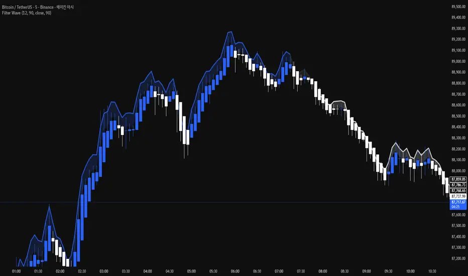
Filter Wave1. Indicator Name
Filter Wave
2. One-line Introduction
A visually enhanced trend strength indicator that uses linear regression scoring to render smoothed, color-shifting waves synced to price action.
3. General Overview
Filter Wave+ is a trend analysis tool designed to provide an intuitive and visually dynamic representation of market momentum.
It uses a pairwise comparison algorithm on linear regression values over a lookback period to determine whether price action is consistently moving upward or downward.
The result is a trend score, which is normalized and translated into a color-coded wave that floats above or below the current price. The wave's opacity increases with trend strength, giving a visual cue for confidence in the trend.
The wave itself is not a raw line—it goes through a three-stage smoothing process, producing a natural, flowing curve that is aesthetically aligned with price movement.
This makes it ideal for traders who need a quick visual context before acting on signals from other tools.
While Filter Wave+ does not generate buy/sell signals directly, its secure and efficient design allows it to serve as a high-confidence trend filter in any trading system.
4. Key Advantages
🌊 Smooth, Dynamic Wave Output
3-stage smoothed curves give clean, flowing visual feedback on market conditions.
🎨 Trend Strength Visualized by Color Intensity
Stronger trends appear with more solid coloring, while weak/neutral trends fade visually.
🔍 Quantitative Trend Detection
Linear regression ordering delivers precise, math-based trend scoring for confidence assessment.
📊 Price-Synced Floating Wave
Wave is dynamically positioned based on ATR and price to align naturally with market structure.
🧩 Compatible with Any Strategy
No conflicting signals—Filter Wave+ serves as a directional overlay that enhances clarity.
🔒 Secure Core Logic
Core algorithm is lightweight and secure, with minimal code exposure and strong encapsulation.
📘 Indicator User Guide
📌 Basic Concept
Filter Wave+ calculates trend direction and intensity using linear regression alignment over time.
The resulting wave is rendered as a smoothed curve, colored based on trend direction (green for up, red for down, gray for neutral), and adjusted in transparency to reflect trend strength.
This allows for fast trend interpretation without overwhelming the chart with signals.
⚙️ Settings Explained
Lookback Period: Number of bars used for pairwise regression comparisons (higher = smoother detection)
Range Tolerance (%): Threshold to qualify as an up/down trend (lower = more sensitive)
Regression Source: The price input used in regression calculation (default: close)
Linear Regression Length: The period used for the core regression line
Bull/Bear Color: Customize the color for bullish and bearish waves
📈 Timing Example
Wave color changes to green and becomes more visible (less transparent)
Wave floats above price and aligns with an uptrend
Use as trend confirmation when other signals are present
📉 Timing Example
Wave shifts to red and darkens, floating below the price
Regression direction down; price continues beneath the wave
Acts as bearish confirmation for short trades or risk-off positioning
🧪 Recommended Use Cases
Use as a trend confidence overlay on your existing strategies
Especially useful in swing trading for detecting and confirming dominant market direction
Combine with RSI, MACD, or price action for high-accuracy setups
🔒 Precautions
This is not a signal generator—intended as a trend filter or directional guide
May respond slightly slower in volatile reversals; pair with responsive indicators
Wave position is influenced by ATR and price but does not represent exact entry/exit levels
Parameter optimization is recommended based on asset class and timeframe
Filter Bar1. Indicator Name
Filter Bar
2. One-line Introduction
A trend-aware bar coloring system that visualizes market direction and strength through adaptive transparency based on regression scoring.
3. General Overview
Filter Bar+ is a minimalist but powerful trend visualization tool that colors chart bars according to market direction and momentum strength.
It analyzes the linear regression trend alignment over a specified lookback period and uses a pairwise comparison algorithm to determine whether the market is in a bullish, bearish, or neutral state.
The result is a "trend score" that gets normalized to reflect trend intensity (0~1).
Bar colors are then dynamically updated using the specified bullish or bearish base colors, where higher intensity results in more opaque (darker) bars, and weaker trends lead to lighter, faded tones.
If no strong trend is detected, bars are shown in gray, signaling indecision or neutrality.
The strength of this indicator lies in its simplicity—it doesn’t draw lines, waves, or shapes, but overlays insight directly onto the chart through smart color cues.
It’s particularly effective as a background filter for price action traders, scalpers, and anyone who prefers clean charts but still wants embedded directional context.
4. Key Advantages
🎨 Adaptive Bar Coloring
Bar color opacity increases with trend strength, offering instant visual confirmation without clutter.
📊 Quantified Trend Direction
Uses a regression-based scoring system to reliably detect uptrends, downtrends, or sideways markets.
⚖️ Customizable Sensitivity
Parameters like lookback period and tolerance percentage give users full control over signal responsiveness.
🧼 Clean Chart Presentation
No lines, shapes, or overlays—just color-coded bars that blend into your existing chart setup.
🚀 Lightweight & Fast
Minimal computational load ensures it works smoothly even on lower-end devices or multiple chart setups.
🔒 Secure Internal Logic
Algorithm is neatly encapsulated and optimized, with no critical logic exposed.
📘 Indicator User Guide
📌 Basic Concept
Filter Bar+ evaluates trend direction and strength using a pairwise comparison of linear regression values.
The result determines whether the market is bullish, bearish, or neutral, and adjusts bar colors accordingly.
It visually amplifies the current market state without drawing any indicators on the chart.
⚙️ Settings Explained
Lookback Period: Number of bars used to compare regression values
Range Tolerance (%): Minimum score required to label a trend as bullish or bearish
Regression Source: Data input used for regression (default: close)
Linear Regression Length: Period for generating the base regression line
Bull/Bear Base Colors: Choose colors to represent bullish or bearish bars
📈 Buy Timing Example
Bars are green (or user-set bullish color) and becoming more vivid
Indicates a strengthening bullish trend; helpful when used alongside breakout confirmation or support zones
📉 Sell Timing Example
Bars turn red (or your custom bearish color) with increasing opacity
Signals growing bearish pressure; acts as confirmation during short setups or breakdowns
🧪 Recommended Use Cases
Combine with volume, RSI, or price action setups for direction filtering
Ideal for clean chart strategies where visual simplicity is preferred
Use as a confirmation layer to reduce noise in sideways markets
🔒 Precautions
This is a visual filter, not a signal generator—use alongside other strategies for entries/exits
In choppy markets, bars may flicker between colors—adjust sensitivity as needed
Works best when you already have a directional thesis and want to validate it visually
Always test settings for your asset/timeframe before applying in live trades

Static K-means Clustering | InvestorUnknownStatic K-Means Clustering is a machine-learning-driven market regime classifier designed for traders who want a data-driven structure instead of subjective indicators or manually drawn zones.
This script performs offline (static) K-means training on your chosen historical window. Using four engineered features:
RSI (Momentum)
CCI (Price deviation / Mean reversion)
CMF (Money flow / Strength)
MACD Histogram (Trend acceleration)
It groups past market conditions into K distinct clusters (regimes). After training, every new bar is assigned to the nearest cluster via Euclidean distance in 4-dimensional standardized feature space.
This allows you to create models like:
Regime-based long/short filters
Volatility phase detectors
Trend vs. chop separation
Mean-reversion vs. breakout classification
Volume-enhanced money-flow regime shifts
Full machine-learning trading systems based solely on regimes
Note:
This script is not a universal ML strategy out of the box.
The user must engineer the feature set to match their trading style and target market.
K-means is a tool, not a ready made system, this script provides the framework.
Core Idea
K-means clustering takes raw, unlabeled market observations and attempts to discover structure by grouping similar bars together.
// STEP 1 — DATA POINTS ON A COORDINATE PLANE
// We start with raw, unlabeled data scattered in 2D space (x/y).
// At this point, nothing is grouped—these are just observations.
// K-means will try to discover structure by grouping nearby points.
//
// y ↑
// |
// 12 | •
// | •
// 10 | •
// | •
// 8 | • •
// |
// 6 | •
// |
// 4 | •
// |
// 2 |______________________________________________→ x
// 2 4 6 8 10 12 14
//
//
//
// STEP 2 — RANDOMLY PLACE INITIAL CENTROIDS
// The algorithm begins by placing K centroids at random positions.
// These centroids act as the temporary “representatives” of clusters.
// Their starting positions heavily influence the first assignment step.
//
// y ↑
// |
// 12 | •
// | •
// 10 | • C2 ×
// | •
// 8 | • •
// |
// 6 | C1 × •
// |
// 4 | •
// |
// 2 |______________________________________________→ x
// 2 4 6 8 10 12 14
//
//
//
// STEP 3 — ASSIGN POINTS TO NEAREST CENTROID
// Each point is compared to all centroids.
// Using simple Euclidean distance, each point joins the cluster
// of the centroid it is closest to.
// This creates a temporary grouping of the data.
//
// (Coloring concept shown using labels)
//
// - Points closer to C1 → Cluster 1
// - Points closer to C2 → Cluster 2
//
// y ↑
// |
// 12 | 2
// | 1
// 10 | 1 C2 ×
// | 2
// 8 | 1 2
// |
// 6 | C1 × 2
// |
// 4 | 1
// |
// 2 |______________________________________________→ x
// 2 4 6 8 10 12 14
//
// (1 = assigned to Cluster 1, 2 = assigned to Cluster 2)
// At this stage, clusters are formed purely by distance.
Your chosen historical window becomes the static training dataset , and after fitting, the centroids never change again.
This makes the model:
Predictable
Repeatable
Consistent across backtests
Fast for live use (no recalculation of centroids every bar)
Static Training Window
You select a period with:
Training Start
Training End
Only bars inside this range are used to fit the K-means model. This window defines:
the market regime examples
the statistical distributions (means/std) for each feature
how the centroids will be positioned post-trainin
Bars before training = fully transparent
Training bars = gray
Post-training bars = full colored regimes
Feature Engineering (4D Input Vector)
Every bar during training becomes a 4-dimensional point:
This combination balances: momentum, volatility, mean-reversion, trend acceleration giving the algorithm a richer "market fingerprint" per bar.
Standardization
To prevent any feature from dominating due to scale differences (e.g., CMF near zero vs CCI ±200), all features are standardized:
standardize(value, mean, std) =>
(value - mean) / std
Centroid Initialization
Centroids start at diverse coordinates using various curves:
linear
sinusoidal
sign-preserving quadratic
tanh compression
init_centroids() =>
// Spread centroids across using different shapes per feature
for c = 0 to k_clusters - 1
frac = k_clusters == 1 ? 0.0 : c / (k_clusters - 1.0) // 0 → 1
v = frac * 2 - 1 // -1 → +1
array.set(cent_rsi, c, v) // linear
array.set(cent_cci, c, math.sin(v)) // sinusoidal
array.set(cent_cmf, c, v * v * (v < 0 ? -1 : 1)) // quadratic sign-preserving
array.set(cent_mac, c, tanh(v)) // compressed
This makes initial cluster spread “random” even though true randomness is hardly achieved in pinescript.
K-Means Iterative Refinement
The algorithm repeats these steps:
(A) Assignment Step, Each bar is assigned to the nearest centroid via Euclidean distance in 4D:
distance = sqrt(dx² + dy² + dz² + dw²)
(B) Update Step, Centroids update to the mean of points assigned to them. This repeats iterations times (configurable).
LIVE REGIME CLASSIFICATION
After training, each new bar is:
Standardized using the training mean/std
Compared to all centroids
Assigned to the nearest cluster
Bar color updates based on cluster
No re-training occurs. This ensures:
No lookahead bias
Clean historical testing
Stable regimes over time
CLUSTER BEHAVIOR & TRADING LOGIC
Clusters (0, 1, 2, 3…) hold no inherent meaning. The user defines what each cluster does.
Example of custom actions:
Cluster 0 → Cash
Cluster 1 → Long
Cluster 2 → Short
Cluster 3+ → Cash (noise regime)
This flexibility means:
One trader might have cluster 0 as consolidation.
Another might repurpose it as a breakout-loading zone.
A third might ignore 3 clusters entirely.
Example on ETHUSD
Important Note:
Any change of parameters or chart timeframe or ticker can cause the “order” of clusters to change
The script does NOT assume any cluster equals any actionable bias, user decides.
PERFORMANCE METRICS & ROC TABLE
The indicator computes average 1-bar ROC for each cluster in:
Training set
Test (live) set
This helps measure:
Cluster profitability consistency
Regime forward predictability
Whether a regime is noise, trend, or reversion-biased
EQUITY SIMULATION & FEES
Designed for close-to-close realistic backtesting.
Position = cluster of previous bar
Fees applied only on regime switches. Meaning:
Staying long → no fee
Switching long→short → fee applied
Switching any→cash → fee applied
Fee input is percentage, but script already converts internally.
Disclaimers
⚠️ This indicator uses machine-learning but does not predict the future. It classifies similarity to past regimes, nothing more.
⚠️ Backtest results are not indicative of future performance.
⚠️ Clusters have no inherent “bullish” or “bearish” meaning. You must interpret them based on your testing and your own feature engineering.

LibVeloLibrary "LibVelo"
This library provides a sophisticated framework for **Velocity
Profile (Flow Rate)** analysis. It measures the physical
speed of trading at specific price levels by relating volume
to the time spent at those levels.
## Core Concept: Market Velocity
Unlike Volume Profiles, which only answer "how much" traded,
Velocity Profiles answer "how fast" it traded.
It is calculated as:
`Velocity = Volume / Duration`
This metric (contracts per second) reveals hidden market
dynamics invisible to pure Volume or TPO profiles:
1. **High Velocity (Fast Flow):**
* **Aggression:** Initiative buyers/sellers hitting market
orders rapidly.
* **Liquidity Vacuum:** Price slips through a level because
order book depth is thin (low resistance).
2. **Low Velocity (Slow Flow):**
* **Absorption:** High volume but very slow price movement.
Indicates massive passive limit orders ("Icebergs").
* **Apathy:** Little volume over a long time. Lack of
interest from major participants.
## Architecture: Triple-Engine Composition
To ensure maximum performance while offering full statistical
depth for all metrics, this library utilises **object
composition** with a lazy evaluation strategy:
#### Engine A: The Master (`vpVol`)
* **Role:** Standard Volume Profile.
* **Purpose:** Maintains the "ground truth" of volume distribution,
price buckets, and ranges.
#### Engine B: The Time Container (`vpTime`)
* **Role:** specialized container for time duration (in ms).
* **Hack:** It repurposes standard volume arrays (specifically
`aBuy`) to accumulate time duration for each bucket.
#### Engine C: The Calculator (`vpVelo`)
* **Role:** Temporary scratchpad for derived metrics.
* **Purpose:** When complex statistics (like Value Area or Skewness)
are requested for **Velocity**, this engine is assembled
on-demand to leverage the full statistical power of `LibVPrf`
without rewriting complex algorithms.
---
**DISCLAIMER**
This library is provided "AS IS" and for informational and
educational purposes only. It does not constitute financial,
investment, or trading advice.
The author assumes no liability for any errors, inaccuracies,
or omissions in the code. Using this library to build
trading indicators or strategies is entirely at your own risk.
As a developer using this library, you are solely responsible
for the rigorous testing, validation, and performance of any
scripts you create based on these functions. The author shall
not be held liable for any financial losses incurred directly
or indirectly from the use of this library or any scripts
derived from it.
create(buckets, rangeUp, rangeLo, dynamic, valueArea, allot, estimator, cdfSteps, split, trendLen)
Construct a new `Velo` controller, initializing its engines.
Parameters:
buckets (int) : series int Number of price buckets ≥ 1.
rangeUp (float) : series float Upper price bound (absolute).
rangeLo (float) : series float Lower price bound (absolute).
dynamic (bool) : series bool Flag for dynamic adaption of profile ranges.
valueArea (int) : series int Percentage for Value Area (1..100).
allot (series AllotMode) : series AllotMode Allocation mode `Classic` or `PDF` (default `PDF`).
estimator (series PriceEst enum from AustrianTradingMachine/LibBrSt/1) : series PriceEst PDF model for distribution attribution (default `Uniform`).
cdfSteps (int) : series int Resolution for PDF integration (default 20).
split (series SplitMode) : series SplitMode Buy/Sell split for the master volume engine (default `Classic`).
trendLen (int) : series int Look‑back for trend factor in dynamic split (default 3).
Returns: Velo Freshly initialised velocity profile.
method clone(self)
Create a deep copy of the composite profile.
Namespace types: Velo
Parameters:
self (Velo) : Velo Profile object to copy.
Returns: Velo A completely independent clone.
method clear(self)
Reset all engines and accumulators.
Namespace types: Velo
Parameters:
self (Velo) : Velo Profile object to clear.
Returns: Velo Cleared profile (chaining).
method merge(self, srcVolBuy, srcVolSell, srcTime, srcRangeUp, srcRangeLo, srcVolCvd, srcVolCvdHi, srcVolCvdLo)
Merges external data (Volume and Time) into the current profile.
Automatically handles resizing and re-bucketing if ranges differ.
Namespace types: Velo
Parameters:
self (Velo) : Velo The profile object.
srcVolBuy (array) : array Source Buy Volume bucket array.
srcVolSell (array) : array Source Sell Volume bucket array.
srcTime (array) : array Source Time bucket array (ms).
srcRangeUp (float) : series float Upper price bound of the source data.
srcRangeLo (float) : series float Lower price bound of the source data.
srcVolCvd (float) : series float Source Volume CVD final value.
srcVolCvdHi (float) : series float Source Volume CVD High watermark.
srcVolCvdLo (float) : series float Source Volume CVD Low watermark.
Returns: Velo `self` (chaining).
method addBar(self, offset)
Main data ingestion. Distributes Volume and Time to buckets.
Namespace types: Velo
Parameters:
self (Velo) : Velo The profile object.
offset (int) : series int Offset of the bar to add (default 0).
Returns: Velo `self` (chaining).
method setBuckets(self, buckets)
Sets the number of buckets for the profile.
Namespace types: Velo
Parameters:
self (Velo) : Velo The profile object.
buckets (int) : series int New number of buckets.
Returns: Velo `self` (chaining).
method setRanges(self, rangeUp, rangeLo)
Sets the price range for the profile.
Namespace types: Velo
Parameters:
self (Velo) : Velo The profile object.
rangeUp (float) : series float New upper price bound.
rangeLo (float) : series float New lower price bound.
Returns: Velo `self` (chaining).
method setValueArea(self, va)
Set the percentage of volume/time for the Value Area.
Namespace types: Velo
Parameters:
self (Velo) : Velo The profile object.
va (int) : series int New Value Area percentage (0..100).
Returns: Velo `self` (chaining).
method getBuckets(self)
Returns the current number of buckets in the profile.
Namespace types: Velo
Parameters:
self (Velo) : Velo The profile object.
Returns: series int The number of buckets.
method getRanges(self)
Returns the current price range of the profile.
Namespace types: Velo
Parameters:
self (Velo) : Velo The profile object.
Returns:
rangeUp series float The upper price bound of the profile.
rangeLo series float The lower price bound of the profile.
method getArrayBuyVol(self)
Returns the internal raw data array for **Buy Volume** directly.
Namespace types: Velo
Parameters:
self (Velo) : Velo The profile object.
Returns: array The internal array for buy volume.
method getArraySellVol(self)
Returns the internal raw data array for **Sell Volume** directly.
Namespace types: Velo
Parameters:
self (Velo) : Velo The profile object.
Returns: array The internal array for sell volume.
method getArrayTime(self)
Returns the internal raw data array for **Time** (in ms) directly.
Namespace types: Velo
Parameters:
self (Velo) : Velo The profile object.
Returns: array The internal array for time duration.
method getArrayBuyVelo(self)
Returns the internal raw data array for **Buy Velocity** directly.
Automatically executes _assemble() if data is dirty.
Namespace types: Velo
Parameters:
self (Velo) : Velo The profile object.
Returns: array The internal array for buy velocity.
method getArraySellVelo(self)
Returns the internal raw data array for **Sell Velocity** directly.
Automatically executes _assemble() if data is dirty.
Namespace types: Velo
Parameters:
self (Velo) : Velo The profile object.
Returns: array The internal array for sell velocity.
method getBucketBuyVol(self, idx)
Returns the **Buy Volume** of a specific bucket.
Namespace types: Velo
Parameters:
self (Velo) : Velo The profile object.
idx (int) : series int The index of the bucket.
Returns: series float The buy volume.
method getBucketSellVol(self, idx)
Returns the **Sell Volume** of a specific bucket.
Namespace types: Velo
Parameters:
self (Velo) : Velo The profile object.
idx (int) : series int The index of the bucket.
Returns: series float The sell volume.
method getBucketTime(self, idx)
Returns the raw accumulated time (in ms) spent in a specific bucket.
Namespace types: Velo
Parameters:
self (Velo) : Velo The profile object.
idx (int) : series int The index of the bucket.
Returns: series float The time in milliseconds.
method getBucketBuyVelo(self, idx)
Returns the **Buy Velocity** (Aggressive Buy Flow) of a bucket.
Namespace types: Velo
Parameters:
self (Velo) : Velo The profile object.
idx (int) : series int The index of the bucket.
Returns: series float The buy velocity in .
method getBucketSellVelo(self, idx)
Returns the **Sell Velocity** (Aggressive Sell Flow) of a bucket.
Namespace types: Velo
Parameters:
self (Velo) : Velo The profile object.
idx (int) : series int The index of the bucket.
Returns: series float The sell velocity in .
method getBktBnds(self, idx)
Returns the price boundaries of a specific bucket.
Namespace types: Velo
Parameters:
self (Velo) : Velo The profile object.
idx (int) : series int The index of the bucket.
Returns:
up series float The upper price bound of the bucket.
lo series float The lower price bound of the bucket.
method getPoc(self, target)
Returns Point of Control (POC) information for the specified target metric.
Calculates on-demand if the target is 'Velocity' and data changed.
Namespace types: Velo
Parameters:
self (Velo) : Velo The profile object.
target (series Metric) : Metric The data aspect to analyse (Volume, Time, Velocity).
Returns:
pocIdx series int The index of the POC bucket.
pocPrice series float The mid-price of the POC bucket.
method getVA(self, target)
Returns Value Area (VA) information for the specified target metric.
Calculates on-demand if the target is 'Velocity' and data changed.
Namespace types: Velo
Parameters:
self (Velo) : Velo The profile object.
target (series Metric) : Metric The data aspect to analyse (Volume, Time, Velocity).
Returns:
vaUpIdx series int The index of the upper VA bucket.
vaUpPrice series float The upper price bound of the VA.
vaLoIdx series int The index of the lower VA bucket.
vaLoPrice series float The lower price bound of the VA.
method getMedian(self, target)
Returns the Median price for the specified target metric distribution.
Calculates on-demand if the target is 'Velocity' and data changed.
Namespace types: Velo
Parameters:
self (Velo) : Velo The profile object.
target (series Metric) : Metric The data aspect to analyse (Volume, Time, Velocity).
Returns:
medianIdx series int The index of the bucket containing the median.
medianPrice series float The median price.
method getAverage(self, target)
Returns the weighted average price (VWAP/TWAP) for the specified target.
Calculates on-demand if the target is 'Velocity' and data changed.
Namespace types: Velo
Parameters:
self (Velo) : Velo The profile object.
target (series Metric) : Metric The data aspect to analyse (Volume, Time, Velocity).
Returns:
avgIdx series int The index of the bucket containing the average.
avgPrice series float The weighted average price.
method getStdDev(self, target)
Returns the standard deviation for the specified target distribution.
Calculates on-demand if the target is 'Velocity' and data changed.
Namespace types: Velo
Parameters:
self (Velo) : Velo The profile object.
target (series Metric) : Metric The data aspect to analyse (Volume, Time, Velocity).
Returns: series float The standard deviation.
method getSkewness(self, target)
Returns the skewness for the specified target distribution.
Calculates on-demand if the target is 'Velocity' and data changed.
Namespace types: Velo
Parameters:
self (Velo) : Velo The profile object.
target (series Metric) : Metric The data aspect to analyse (Volume, Time, Velocity).
Returns: series float The skewness.
method getKurtosis(self, target)
Returns the excess kurtosis for the specified target distribution.
Calculates on-demand if the target is 'Velocity' and data changed.
Namespace types: Velo
Parameters:
self (Velo) : Velo The profile object.
target (series Metric) : Metric The data aspect to analyse (Volume, Time, Velocity).
Returns: series float The excess kurtosis.
method getSegments(self, target)
Returns the fundamental unimodal segments for the specified target metric.
Calculates on-demand if the target is 'Velocity' and data changed.
Namespace types: Velo
Parameters:
self (Velo) : Velo The profile object.
target (series Metric) : Metric The data aspect to analyse (Volume, Time, Velocity).
Returns: matrix A 2-column matrix where each row is an pair.
method getCvd(self, target)
Returns Cumulative Volume/Velo Delta (CVD) information for the target metric.
Namespace types: Velo
Parameters:
self (Velo) : Velo The profile object.
target (series Metric) : Metric The data aspect to analyse (Volume, Time, Velocity).
Returns:
cvd series float The final delta value.
cvdHi series float The historical high-water mark of the delta.
cvdLo series float The historical low-water mark of the delta.
Velo
Velo Composite Velocity Profile Controller.
Fields:
_vpVol (VPrf type from AustrianTradingMachine/LibVPrf/2) : LibVPrf.VPrf Engine A: Master Volume source.
_vpTime (VPrf type from AustrianTradingMachine/LibVPrf/2) : LibVPrf.VPrf Engine B: Time duration container (ms).
_vpVelo (VPrf type from AustrianTradingMachine/LibVPrf/2) : LibVPrf.VPrf Engine C: Scratchpad for velocity stats.
_aTime (array) : array Pointer alias to `vpTime.aBuy` (Time storage).
_valueArea (series float) : int Percentage of total volume to include in the Value Area (1..100)
_estimator (series PriceEst enum from AustrianTradingMachine/LibBrSt/1) : LibBrSt.PriceEst PDF model for distribution attribution.
_allot (series AllotMode) : AllotMode Attribution model (Classic or PDF).
_cdfSteps (series int) : int Integration resolution for PDF.
_isDirty (series bool) : bool Lazy evaluation flag for vpVelo.

RastaRasta — Educational Strategy (Pine v5)
Momentum · Smoothing · Trend Study
Overview
The Rasta Strategy is a visual and educational framework designed to help traders study momentum transitions using the interaction between a fast-reacting EMA line and a slower smoothed reference line.
It is not a signal generator or profit system; it’s a learning tool for understanding how smoothing, crossovers, and filters interact under different market conditions.
The script displays:
A primary EMA line (the fast reactive wave).
A Smoothed line (using your chosen smoothing method).
Optional fog zones between them for quick visual context.
Optional DNA rungs connecting both lines to illustrate volatility compression and expansion.
Optional EMA 8 / EMA 21 trend filter to observe higher-time-frame alignment.
Core Idea
The Rasta model focuses on wave interaction. When the fast EMA crosses above the smoothed line, it reflects a shift in short-term momentum relative to background trend pressure. Cross-unders suggest weakening or reversal.
Rather than treating this as a trading “signal,” use it to observe structure, study trend alignment, and test how smoothing type affects reaction speed.
Smoothing Types Explained
The script lets you experiment with multiple smoothing techniques:
Type Description Use Case
SMA (Simple Moving Average) Arithmetic mean of the last n values. Smooth and steady, but slower. Trend-following studies; filters noise on higher time frames.
EMA (Exponential Moving Average) Weights recent data more. Responds faster to new price action. Momentum or reactive strategies; quick shifts and reversals.
RMA (Relative Moving Average) Used internally by RSI; smooths exponentially but slower than EMA. Momentum confirmation; balanced response.
WMA (Weighted Moving Average) Linear weights emphasizing the most recent data strongly. Intraday scalping; crisp but potentially noisy.
None Disables smoothing; uses the EMA line alone. Raw comparison baseline.
Each smoothing method changes how early or late the strategy reacts:
Faster smoothing (EMA/WMA) = more responsive, good for scalping.
Slower smoothing (SMA/RMA) = more stable, good for trend following.
Modes of Study
🔹 Scalper Mode
Use short EMA lengths (e.g., 3–5) and fast smoothing (EMA or WMA).
Focus on 1 min – 15 min charts.
Watch how quick crossovers appear near local tops/bottoms.
Fog and rung compression reveal volatility contraction before bursts.
Goal: study short-term rhythm and liquidity pulses.
🔹 Momentum Mode
Use moderate EMA (5–9) and RMA smoothing.
Ideal for 1 H–4 H charts.
Observe how the fog color aligns with trend shifts.
EMA 8 / 21 filter can act as macro bias; “Enter” labels will appear only in its direction when enabled.
Goal: study sustained motion between pullbacks and acceleration waves.
🔹 Trend-Follower Mode
Use longer EMA (13–21) with SMA smoothing.
Great for daily/weekly charts.
Focus on periods where fog stays unbroken for long stretches — these illustrate clear trend dominance.
Watch rung spacing: tight clusters often precede consolidations; wide rungs signal expanding volatility.
Goal: visualize slow-motion trend transitions and filter whipsaw conditions.
Components
EMA Line (Red): Fast-reacting short-term direction.
Smoothed Line (Yellow): Reference trend baseline.
Fog Zone: Green when EMA > Smoothed (up-momentum), red when below.
DNA Rungs: Thin connectors showing volatility structure.
EMA 8 / 21 Filter (optional):
When enabled, the strategy will only allow Enter events if EMA 8 > EMA 21.
Use this to study higher-trend gating effects.
Educational Applications
Momentum Visualization: Observe how the fast EMA “breathes” around the smoothed baseline.
Trend Transitions: Compare different smoothing types to see how early or late reversals are detected.
Noise Filtering: Experiment with fog opacity and smoothing lengths to understand trade-off between responsiveness and stability.
Risk Concept Simulation: Includes a simple fixed stop-loss parameter (default 13%) for educational demonstrations of position management in the Strategy Tester.
How to Use
Add to Chart → “Strategy.”
Works on any timeframe and instrument.
Adjust Parameters:
Length: base EMA speed.
Smoothing Type: choose SMA, EMA, RMA, or WMA.
Smoothing Length: controls delay and smoothness.
EMA 8 / 21 Filter: toggles trend gating.
Fog & Rungs: visual study options only.
Study Behavior:
Use Strategy Tester → List of Trades for entry/exit context.
Observe how different smoothing types affect early vs. late “Enter” points.
Compare trend periods vs. ranging periods to evaluate efficiency.
Combine with External Tools:
Overlay RSI, MACD, or Volume for deeper correlation analysis.
Use replay mode to visualize crossovers in live sequence.
Interpreting the Labels
Enter: Marks where fast EMA crosses above the smoothed line (or when filter flips positive).
Exit: Marks where fast EMA crosses back below.
These are purely analytical markers — they do not represent trade advice.
Educational Value
The Rasta framework helps learners explore:
Reaction time differences between moving-average algorithms.
Impact of smoothing on signal clarity.
Interaction of local and global trends.
Visualization of volatility contraction (tight DNA rungs) and expansion (wide fog zones).
It’s a sandbox for studying price structure, not a promise of profit.
Disclaimer
This script is provided for educational and research purposes only.
It does not constitute financial advice, trading signals, or performance guarantees. Past market behavior does not predict future outcomes.
Users are encouraged to experiment responsibly, record observations, and develop their own understanding of price behavior.
Author: Michael Culpepper (mikeyc747)
License: Educational / Open for study and modification with credit.
Philosophy:
“Learning the rhythm of the market is more valuable than chasing its profits.” — Rasta

[FS] Pivot Measurements# Pivot Measurements
An advanced TradingView indicator that combines LuxAlgo's pivot point detection algorithm with automatic measurement calculations between consecutive pivots.
## Features
### Pivot Detection
- **Regular Pivots**: Detects standard pivot highs and lows using configurable pivot length
- **Missed Pivots**: Identifies missed reversal levels that occurred between regular pivots
- **Visual Indicators**:
- Regular pivot highs: Red downward triangle (▼)
- Regular pivot lows: Teal upward triangle (▲)
- Missed pivots: Ghost emoji (👻)
- **Zigzag Lines**: Connects pivots with colored lines (solid for regular, dashed for missed)
- **Ghost Levels**: Horizontal lines indicating missed pivot levels
### Measurement System
- **Automatic Measurements**: Calculates price movements between consecutive pivots
- **Visual Display**:
- Transparent colored boxes (blue for upward, red for downward movements)
- Measurement labels showing:
- Price change (absolute and percentage)
- Duration (bars, days, hours, minutes)
- Volume approximation
- **Smart Positioning**: Labels positioned outside boxes (above for upward, below for downward)
- **Color Coding**: Blue for positive movements, red for negative movements
## Parameters
### Pivot Detection
- **Pivot Length** (default: 50): Number of bars on each side to identify a pivot point
- **Regular Pivots**: Toggle and colors for regular pivot highs and lows
- **Missed Pivots**: Toggle and colors for missed pivot detection
### Measurements
- **Number of Measurements** (1-10, default: 10): Maximum number of measurements to display
- **Show Measurement Boxes**: Toggle to show/hide measurement boxes and labels
- **Box Transparency** (0-100, default: 90): Transparency level for measurement boxes
- **Border Transparency** (0-100, default: 50): Transparency level for box borders
- **Label Background Transparency** (0-100, default: 30): Transparency level for label backgrounds
- **Label Size**: Size of measurement labels (tiny, small, normal, large)
## Usage
1. Add the indicator to your chart
2. Configure the **Pivot Length** based on your timeframe:
- Lower values for shorter timeframes (e.g., 10-20 for 1-5 min)
- Higher values for longer timeframes (e.g., 50-100 for daily)
3. Adjust pivot colors and visibility as needed
4. Customize measurement display settings:
- Set the number of measurements to display
- Adjust transparency levels for boxes, borders, and labels
- Choose label size
## Technical Details
- **Pine Script Version**: v6
- **Pivot Detection**: Based on () algorithm for detecting regular and missed pivots
- **Measurement Calculation**:
- Measures between consecutive pivots (from most recent to older)
- Calculates price change, percentage change, duration, and approximate volume
- Automatically sorts pivots chronologically
- **Performance**: Optimized with helper functions to reduce code duplication
## Notes
- The indicator automatically limits the number of stored pivots to optimize performance
- Measurements are only created when there are at least 2 pivots detected
- All measurements are recalculated on each bar update
- The indicator uses `max_bars_back=5000` to ensure sufficient historical data
## License
This indicator uses LuxAlgo's pivot detection algorithm from (). Please refer to the original LuxAlgo license for pivot detection components.

Smart Flow Tracker [The_lurker]
Smart Flow Tracker (SFT): Advanced Order Flow Tracking Indicator
Overview
Smart Flow Tracker (SFT) is an advanced indicator designed for real-time tracking and analysis of order flows. It focuses on detecting institutional patterns, massive orders, and potential reversals through analysis of lower timeframes (Lower Timeframe) or live ticks. It provides deep insights into market behavior using a multi-layered intelligent detection system and a clear visual interface, giving traders a competitive edge.
SFT focuses on trade volumes, directions, and frequencies to uncover unusual activity that may indicate institutional intervention, massive orders, or manipulation attempts (traps).
Indicator Operation Levels
SFT operates on three main levels:
1. Microscopic Monitoring: Tracks every trade at precise timeframes (down to one second), providing visibility not available in standard timeframes.
2. Advanced Statistical Analysis: Calculates averages, deviations, patterns, and anomalies using precise mathematical algorithms.
3. Behavioral Artificial Intelligence: Recognizes behavioral patterns such as hidden institutional accumulation, manipulation attempts and traps, and potential reversal points.
Key Features
SFT features a set of advanced functions to enhance the trader's experience:
1. Intelligent Order Classification System: Classifies orders into six categories based on size and pattern:
- Standard: Normal orders with typical size.
- Significant 💎: Orders larger than average by 1.5 times.
- Major 🔥: Orders larger than average by 2.5 times.
- Massive 🐋: Orders larger than average by 3 times.
- Institutional 🏛️: Consistent patterns indicating institutional activity.
- Reversal 🔄: Large orders indicating direction change.
- Trap ⚠️: Patterns that may be price traps.
2. Institutional Patterns Detection: Tracks sequences of similar-sized orders, detects organized institutional activity, and is customizable (number of trades, variance ratio).
3. Reversals Detection: Compares recent flows with previous ones, detects direction shifts from up to down or vice versa, and operates only on large orders (Major/Massive/Institutional).
4. Traps Detection: Identifies sequences of large orders in one direction, followed by an institutional order in the opposite direction, with early alerts for false moves.
5. Flow Delta Bar: Displays the difference between buy and sell volumes as a percentage for balance, with instant updates per trade.
6. Dynamic Statistics Panel: Displays overall buy and sell ratios with real-time updates and interactive colors.
How It Works and Understanding
SFT relies on logical sequential stages for data processing:
A. Data Collection: Uses the `request.security_lower_tf()` function to extract data from a lower timeframe (like 1S) even on a higher timeframe (like 5D). For each time unit, it calculates:
- Adjusted Volume: Either normal volume or "price-weighted volume" (hlc3 * volume) based on user choice.
- Trade Direction: Compared to previous close (rise → buy, fall → sell).
B. Building Temporary Memory: Maintains a dynamic list (sizeHistory) of the last 100 trade sizes, continuously calculating the moving average (meanSize).
C. Intelligent Classification: Compares each new trade to the average:
- > 1.5 × average → Significant.
- > 2.5 × average → Major.
- > 3.0 × average → Massive.
- Institutional Patterns Check: A certain number of trades (e.g., 5) with a specified variance ratio (±5%) → Institutional.
D. Advanced Detection:
- Reversal: Compares buy/sell totals in two consecutive periods.
- Trap: Sequence of large trades in one direction followed by an opposite institutional trade.
E. Display and Alerts: Results displayed in an automatically updated table, with option to enable alerts for notable events.
Settings (Fully Customizable)
SFT offers extensive options to adapt to the trader's needs:
A. Display Settings:
- Language: English / Arabic.
- Table Position: 9 options (e.g., Top Right, Middle Right, Bottom Left).
- Display Size: Tiny / Small / Normal / Large.
- Max Rows: 10–100.
- Enable Flow Delta Bar: Yes / No.
- Enable Statistics Panel: Yes / No (displays buy/sell % ratio).
B.- Technical Settings:
- Data Source: Lower Timeframe / Live Tick (simulation).
- Timeframe: Optional (e.g., 1S, 5S, 1).
- Calculation Type: Volume / Price Volume.
C. Intelligent Detection System:
- Enable Institutional Patterns Detection.
- Pattern Length: 3–20 trades.
- Allowed Variance Ratio: 1%–20%.
- Massive Orders Detection Factor: 2.0–10.0.
D. Classification Criteria:
- Significant Orders Factor: 1.2–3.0.
- Major Orders Factor: 2.0–5.0.
E. **Advanced Detection**:
- Enable Reversals Detection (with review period).
- Enable Traps Detection (with minimum sequence limit).
F. Alerts System:
- Enable for each type: Massive orders, institutional patterns, reversals, traps, severe imbalance (60%–90%).
G. Color System: Manual customization for each category:
- Standard Buy 🟢: Dark gray green.
- Standard Sell 🔴: Dark gray red.
- Significant Buy 🟢: Medium green.
- Significant Sell 🔴: Medium red.
- Major Orders 🟣: Purple.
- Massive Orders 🟠: Orange.
- Institutional 🟦: Sky blue.
- Reversal 🔵: Blue.
- Trap 🟣: Pink-purple.
Target Audiences
SFT benefits a wide range of traders and investors:
1. Scalpers: Instant detection of large orders, liquidity points identification, avoiding traps in critical moments.
2. Day Traders: Tracking smart money footprint, determining real session direction, early reversals detection.
3. Swing Traders: Confirming trend strength, detecting institutional accumulation/distribution, identifying optimal entry points.
4. Investors: Understanding true market sentiments, avoiding entry at false peaks, identifying real value zones.
⚠️ Disclaimer:
This indicator is for educational and analytical purposes only. It does not constitute financial, investment, or trading advice. Use it in conjunction with your own strategy and risk management. Neither TradingView nor the developer is liable for any financial decisions or losses.
Smart Flow Tracker (SFT): مؤشر متقدم لتتبع تدفقات الأوامر
نظرة عامة
Smart Flow Tracker (SFT) مؤشر متقدم مصمم لتتبع وتحليل تدفقات الأوامر في الوقت الفعلي. يركز على كشف الأنماط المؤسسية، الأوامر الضخمة، والانعكاسات المحتملة من خلال تحليل الأطر الزمنية الأقل (Lower Timeframe) أو التيك الحي. يوفر رؤية عميقة لسلوك السوق باستخدام نظام كشف ذكي متعدد الطبقات وواجهة مرئية واضحة، مما يمنح المتداولين ميزة تنافسية.
يركز SFT على حجم الصفقات، اتجاهها، وتكرارها لكشف النشاط غير العادي الذي قد يشير إلى تدخل مؤسسات، أوامر ضخمة، أو محاولات تلاعب (فخاخ).
مستويات عمل المؤشر
يعمل SFT على ثلاثة مستويات رئيسية:
1. المراقبة المجهرية: يتتبع كل صفقة على مستوى الأطر الزمنية الدقيقة (حتى الثانية الواحدة)، مما يوفر رؤية غير متوفرة في الأطر الزمنية العادية.
2. التحليل الإحصائي المتقدم: يحسب المتوسطات، الانحرافات، الأنماط، والشذوذات باستخدام خوارزميات رياضية دقيقة.
3. الذكاء الاصطناعي السلوكي: يتعرف على أنماط سلوكية مثل التراكم المؤسسي المخفي، محاولات التلاعب والفخاخ، ونقاط الانعكاس المحتملة.
الميزات الرئيسية
يتميز SFT بمجموعة من الوظائف المتقدمة لتحسين تجربة المتداول:
1. نظام تصنيف الأوامر الذكي: يصنف الأوامر إلى ست فئات بناءً على الحجم والنمط:
- Standard (قياسي)**: أوامر عادية بحجم طبيعي.
- Significant 💎 (مهم)**: أوامر أكبر من المتوسط بـ1.5 ضعف.
- Major 🔥 (كبير)**: أوامر أكبر من المتوسط بـ2.5 ضعف.
- Massive 🐋 (ضخم)**: أوامر أكبر من المتوسط بـ3 أضعاف.
- Institutional 🏛️ (مؤسسي)**: أنماط متسقة تشير إلى نشاط مؤسسي.
- Reversal 🔄 (انعكاس)**: أوامر كبيرة تشير إلى تغيير اتجاه.
- Trap ⚠️ (فخ)**: أنماط قد تكون فخاخًا سعرية.
2. كشف الأنماط المؤسسية: يتتبع تسلسل الأوامر المتشابهة في الحجم، يكشف النشاط المؤسسي المنظم، وقابل للتخصيص (عدد الصفقات، نسبة التباين).
3. كشف الانعكاسات: يقارن التدفقات الأخيرة بالسابقة، يكشف تحول الاتجاه من صعود إلى هبوط أو العكس، ويعمل فقط على الأوامر الكبيرة (Major/Massive/Institutional).
4. كشف الفخاخ: يحدد تسلسل أوامر كبيرة في اتجاه واحد، يليها أمر مؤسسي في الاتجاه المعاكس، مع تنبيه مبكر للحركات الكاذبة.
5. شريط دلتا التدفق: يعرض الفرق بين حجم الشراء والبيع كنسبة مئوية للتوازن، مع تحديث فوري لكل صفقة.
6. لوحة إحصائيات ديناميكية: تعرض نسبة الشراء والبيع الإجمالية مع تحديث لحظي وألوان تفاعلية.
طريقة العمل والفهم
يعتمد SFT على مراحل منطقية متسلسلة لمعالجة البيانات:
أ. جمع البيانات: يستخدم دالة `request.security_lower_tf()` لاستخراج بيانات من إطار زمني أدنى (مثل 1S) حتى على إطار زمني أعلى (مثل 5D). لكل وحدة زمنية، يحسب:
- الحجم المعدّل: إما الحجم العادي (volume) أو "الحجم المرجّح بالسعر" (hlc3 * volume) حسب الاختيار.
- اتجاه الصفقة: مقارنة الإغلاق الحالي بالسابق (ارتفاع → شراء، انخفاض → بيع).
ب. بناء الذاكرة المؤقتة: يحتفظ بقائمة ديناميكية (sizeHistory) لآخر 100 حجم صفقة، ويحسب المتوسط المتحرك (meanSize) باستمرار.
ج. التصنيف الذكي: يقارن كل صفقة جديدة بالمتوسط:
- > 1.5 × المتوسط → Significant.
- > 2.5 × المتوسط → Major.
- > 3.0 × المتوسط → Massive.
- فحص الأنماط المؤسسية: عدد معين من الصفقات (مثل 5) بنسبة تباين محددة (±5%) → Institutional.
د. الكشف المتقدم:
- الانعكاس: مقارنة مجموع الشراء/البيع في فترتين متتاليتين.
- الفخ: تسلسل صفقات كبيرة في اتجاه واحد يتبعها صفقة مؤسسية معاكسة.
هـ. العرض والتنبيه: عرض النتائج في جدول محدّث تلقائيًا، مع إمكانية تفعيل تنبيهات للأحداث المميزة.
لإعدادات (قابلة للتخصيص بالكامل)
يوفر SFT خيارات واسعة للتكييف مع احتياجات المتداول:
أ. إعدادات العرض:
- اللغة: English / العربية.
- موقع الجدول: 9 خيارات (مثل Top Right, Middle Right, Bottom Left).
- حجم العرض: Tiny / Small / Normal / Large.
- الحد الأقصى للصفوف: 10–100.
- تفعيل شريط دلتا التدفق: نعم / لا.
- تفعيل لوحة الإحصائيات: نعم / لا (تعرض نسبة الشراء/البيع %).
ب. الإعدادات التقنية:
- مصدر البيانات: Lower Timeframe / Live Tick (محاكاة).
- الإطار الزمني: اختياري (مثل 1S, 5S, 1).
- نوع الحساب: Volume / Price Volume.
ج. نظام الكشف الذكي:
- تفعيل كشف الأنماط المؤسسية.
- طول النمط: 3–20 صفقة.
- نسبة التباين: 1%–20%.
- عامل كشف الأوامر الضخمة: 2.0–10.0.
د. معايير التصنيف:
- عامل الأوامر المهمة: 1.2–3.0.
- عامل الأوامر الكبرى: 2.0–5.0.
هـ. الكشف المتقدم:
- تفعيل كشف الانعكاسات (مع فترة مراجعة).
- تفعيل كشف الفخاخ (مع حد أدنى للتسلسل).
و. نظام التنبيهات:
- تفعيل لكل نوع: أوامر ضخمة، أنماط مؤسسية، انعكاسات، فخاخ، عدم توازن شديد (60%–90%).
ز. نظام الألوان**: تخصيص يدوي لكل فئة:
- شراء قياسي 🟢: أخضر رمادي داكن.
- بيع قياسي 🔴: أحمر رمادي داكن.
- شراء مهم 🟢: أخضر متوسط.
- بيع مهم 🔴: أحمر متوسط.
- أوامر كبرى 🟣: بنفسجي.
- أوامر ضخمة 🟠: برتقالي.
- مؤسسي 🟦: أزرق سماوي.
- انعكاس 🔵: أزرق.
- فخ 🟣: وردي-أرجواني.
الفئات المستهدفة
يستفيد من SFT مجموعة واسعة من المتداولين والمستثمرين:
1. السكالبرز (Scalpers): كشف لحظي للأوامر الكبيرة، تحديد نقاط السيولة، تجنب الفخاخ في اللحظات الحرجة.
2. المتداولون اليوميون (Day Traders): تتبع بصمة الأموال الذكية، تحديد اتجاه الجلسة الحقيقي، كشف الانعكاسات المبكرة.
3. المتداولون المتأرجحون (Swing Traders): تأكيد قوة الاتجاه، كشف التراكم/التوزيع المؤسسي، تحديد نقاط الدخول المثلى.
4. المستثمرون: فهم معنويات السوق الحقيقية، تجنب الدخول في قمم كاذبة، تحديد مناطق القيمة الحقيقية.
⚠️ إخلاء مسؤولية:
هذا المؤشر لأغراض تعليمية وتحليلية فقط. لا يُمثل نصيحة مالية أو استثمارية أو تداولية. استخدمه بالتزامن مع استراتيجيتك الخاصة وإدارة المخاطر. لا يتحمل TradingView ولا المطور مسؤولية أي قرارات مالية أو خسائر.

Smart Money Flow Index (SMFI) - Advanced SMC [PhenLabs]📊Smart Money Flow Index (SMFI)
Version: PineScript™v6
📌Description
The Smart Money Flow Index (SMFI) is an advanced Smart Money Concepts implementation that tracks institutional trading behavior through multi-dimensional analysis. This comprehensive indicator combines volume-validated Order Block detection, Fair Value Gap identification with auto-mitigation tracking, dynamic Liquidity Zone mapping, and Break of Structure/Change of Character detection into a unified system.
Unlike basic SMC indicators, SMFI employs a proprietary scoring algorithm that weighs five critical factors: Order Block strength (validated by volume), Fair Value Gap size and recency, proximity to Liquidity Zones, market structure alignment (BOS/CHoCH), and multi-timeframe confluence. This produces a Smart Money Score (0-100) where readings above 70 represent optimal institutional setup conditions.
🚀Points of Innovation
Volume-Validated Order Block Detection – Only displays Order Blocks when formation candle exceeds customizable volume multiplier (default 1.5x average), filtering weak zones and highlighting true institutional accumulation/distribution
Auto-Mitigation Tracking System – Fair Value Gaps and Order Blocks automatically update status when price mitigates them, with visual distinction between active and filled zones preventing trades on dead levels
Proprietary Smart Money Score Algorithm – Combines weighted factors (OB strength 25%, FVG proximity 20%, Liquidity 20%, Structure 20%, MTF 15%) into single 0-100 confidence rating updating in real-time
ATR-Based Adaptive Calculations – All distance measurements use 14-period Average True Range ensuring consistent function across any instrument, timeframe, or volatility regime without manual recalibration
Dynamic Age Filtering – Automatically removes liquidity levels and FVGs older than configurable thresholds preventing chart clutter while maintaining relevant levels
Multi-Timeframe Confluence Integration – Analyzes higher timeframe bias with customizable multipliers (2-10x) and incorporates HTF trend direction into Smart Money Score for institutional alignment
🔧Core Components
Order Block Engine – Detects institutional supply/demand zones using characteristic patterns (down-move-then-strong-up for bullish, up-move-then-strong-down for bearish) with minimum volume threshold validation, tracks mitigation when price closes through zones
Fair Value Gap Scanner – Identifies price imbalances where current candle's low/high leaves gap with two-candle-prior high/low, filters by minimum size percentage, monitors 50% fill for mitigation status
Liquidity Zone Mapper – Uses pivot high/low detection with configurable lookback to mark swing points where stop losses cluster, extends horizontal lines to visualize sweep targets, manages lifecycle through age-based removal
Market Structure Analyzer – Tracks pivot progression to identify trend through higher-highs/higher-lows (bullish) or lower-highs/lower-lows (bearish), detects Break of Structure and Change of Character for trend/reversal confirmation
Scoring Calculation Engine – Evaluates proximity to nearest Order Blocks using ATR-normalized distance, assesses FVG recency and distance, calculates liquidity proximity with age weighting, combines structure bias and MTF trend into smoothed final score
🔥Key Features
Customizable Display Limits – Control maximum Order Blocks (1-10), Liquidity Zones (1-10), and FVG age (10-200 bars) to maintain clean charts focused on most relevant institutional levels
Gradient Strength Visualization – All zones render with transparency-adjustable coloring where stronger/newer zones appear more solid and weaker/older zones fade progressively providing instant visual hierarchy
Educational Label System – Optional labels identify each zone type (Bullish OB, Bearish OB, Bullish FVG, Bearish FVG, BOS) with color-coded text helping traders learn SMC concepts through practical application
Real-Time Smart Money Score Dashboard – Top-right table displays current score (0-100) with color coding (green >70, yellow 30-70, red <30) plus trend arrow for at-a-glance confidence assessment
Comprehensive Alert Suite – Configurable notifications for Order Block formation, Fair Value Gap detection, Break of Structure events, Change of Character signals, and high Smart Money Score readings (>70)
Buy/Sell Signal Integration – Automatically plots triangle markers when Smart Money Score exceeds 70 with aligned market structure and fresh Order Block detection providing clear entry signals
🎨Visualization
Order Block Boxes – Shaded rectangles extend from formation bar spanning high-to-low of institutional candle, bullish zones in green, bearish in red, with customizable transparency (80-98%)
Fair Value Gap Zones – Rectangular areas marking imbalances, active FVGs display in bright colors with adjustable transparency, mitigated FVGs switch to gray preventing trades on filled zones
Liquidity Level Lines – Dashed horizontal lines extend from pivot creation points, swing highs in bearish color (short targets above), swing lows in bullish color (long targets below), opacity decreases with age
Structure Labels – "BOS" labels appear above/below price when Break of Structure confirmed, colored by direction (green bullish, red bearish), positioned at 1% beyond highs/lows for visibility
Educational Info Panel – Bottom-right table explains key terminology (OB, FVG, BOS, CHoCH) and score interpretation (>70 high probability) with semi-transparent background for readability
📖Usage Guidelines
General Settings
Show Order Blocks – Default: On, toggles visibility of institutional supply/demand zones, disable when focusing solely on FVGs or Liquidity
Show Fair Value Gaps – Default: On, controls FVG zone display including active and mitigated imbalances
Show Liquidity Zones – Default: On, manages liquidity line visibility, disable on lower timeframes to reduce clutter
Show Market Structure – Default: On, toggles BOS/CHoCH label display
Show Smart Money Score – Default: On, controls score dashboard visibility
Order Block Settings
OB Lookback Period – Default: 20, Range: 5-100, controls bars scanned for Order Block patterns, lower values detect recent activity, higher values find older blocks
Min Volume Multiplier – Default: 1.5, Range: 1.0-5.0, sets minimum volume threshold as multiple of 20-period average, higher values (2.0+) filter for strongest institutional candles
Max Order Blocks to Display – Default: 3, Range: 1-10, limits simultaneous Order Blocks shown, lower settings (1-3) maintain focus on most recent zones
Fair Value Gap Settings
Min FVG Size (%) – Default: 0.3, Range: 0.1-2.0, defines minimum gap size as percentage of close price, lower values detect micro-imbalances, higher values focus on significant gaps
Max FVG Age (bars) – Default: 50, Range: 10-200, removes FVGs older than specified bars, lower settings (10-30) for scalping, higher (100-200) for swing trading
Show FVG Mitigation – Default: On, displays filled FVGs in gray providing visual history, disable to show only active untouched imbalances
Liquidity Zone Settings
Liquidity Lookback – Default: 50, Range: 20-200, sets pivot detection period for swing highs/lows, lower values (20-50) mark shorter-term liquidity, higher (100-200) identify major swings
Max Liquidity Age (bars) – Default: 100, Range: 20-500, removes liquidity lines older than specified bars, adjust based on timeframe
Liquidity Sensitivity – Default: 0.5, Range: 0.1-1.0, controls pivot detection sensitivity, lower values mark only major swings, higher values identify minor swings
Max Liquidity Zones to Display – Default: 3, Range: 1-10, limits total liquidity levels shown maintaining chart clarity
Market Structure Settings
Pivot Length – Default: 5, Range: 3-15, defines bars to left/right for pivot validation, lower values (3-5) create sensitive structure breaks, higher (10-15) filter for major shifts
Min Structure Move (%) – Default: 1.0, Range: 0.1-5.0, sets minimum percentage move required between pivots to confirm structure change
Multi-Timeframe Settings
Enable MTF Analysis – Default: On, activates higher timeframe trend analysis incorporation into Smart Money Score
Higher Timeframe Multiplier – Default: 4, Range: 2-10, multiplies current timeframe to determine analysis timeframe (4x on 15min = 1hour)
Visual Settings
Bullish Color – Default: Green (#089981), sets color for bullish Order Blocks, FVGs, and structure elements
Bearish Color – Default: Red (#f23645), defines color for bearish elements
Neutral Color – Default: Gray (#787b86), controls color of mitigated zones and neutral elements
Show Educational Labels – Default: On, displays text labels on zones identifying type (OB, FVG, BOS), disable once familiar with patterns
Order Block Transparency – Default: 92, Range: 80-98, controls Order Block box transparency
FVG Transparency – Default: 92, Range: 80-98, sets Fair Value Gap zone transparency independently from Order Blocks
Alert Settings
Alert on Order Block Formation – Default: On, triggers notification when new volume-validated Order Block detected
Alert on FVG Formation – Default: On, sends alert when Fair Value Gap appears enabling quick response to imbalances
Alert on Break of Structure – Default: On, notifies when BOS or CHoCH confirmed
Alert on High Smart Money Score – Default: On, alerts when Smart Money Score crosses above 70 threshold indicating high-probability setup
✅Best Use Cases
Order Block Retest Entries – After Break of Structure, wait for price retrace into fresh bullish Order Block with Smart Money Score >70, enter long on zone reaction targeting next liquidity level
Fair Value Gap Retracement Trading – When price creates FVG during strong move then retraces, enter as price approaches unfilled gap expecting institutional orders to continue trend
Liquidity Sweep Reversals – Monitor price approaching swing high/low liquidity zones against prevailing Smart Money Score trend, after stop hunt sweep watch for rejection into premium Order Block/FVG
Multi-Timeframe Confluence Setups – Identify alignment when current timeframe Order Block coincides with higher timeframe FVG plus MTF analysis showing matching trend bias
Break of Structure Continuations – After BOS confirms trend direction, trade pullbacks to nearest Order Block or FVG in direction of structure break using Smart Money Score >70 as entry filter
Change of Character Reversal Plays – When CHoCH detected indicating potential reversal, look for Smart Money Score pivot with opposing Order Block formation then enter on structure confirmation
⚠️Limitations
Lagging Pivot Calculations – Pivot-based features (Liquidity Zones, Market Structure) require bars to right of pivot for confirmation, meaning these elements identify levels retrospectively with delay equal to lookback period
Whipsaw in Ranging Markets – During choppy conditions, Order Blocks fail frequently and structure breaks produce false signals as Smart Money Score fluctuates without clear institutional bias, best used in trending markets
Volume Data Dependency – Order Block volume validation requires accurate volume data which may be incomplete on Forex pairs or limited in crypto exchange feeds
Subjectivity in Scoring Weights – Proprietary 25-20-20-20-15 weighting reflects general institutional behavior but may not optimize for specific instruments or market regimes, user cannot adjust factor weights
Visual Complexity on Lower Timeframes – Sub-hour timeframes generate excessive zones creating cluttered charts, requires aggressive display limit reduction and higher minimum thresholds
No Fundamental Integration – Indicator analyzes purely technical price action and volume without incorporating economic events, news catalysts, or fundamental shifts that override technical levels
💡What Makes This Unique
Unified SMC Ecosystem – Unlike indicators displaying Order Blocks OR FVGs OR Liquidity separately, SMFI combines all three institutional concepts plus market structure into single cohesive system
Proprietary Confidence Scoring – Rather than manual setup assessment, automated Smart Money Score quantifies probability by weighting five institutional dimensions into actionable 0-100 rating
Volume-Filtered Quality – Eliminates weak Order Blocks forming without institutional volume confirmation, ensuring displayed zones represent genuine accumulation/distribution
Adaptive Lifecycle Management – Automatically updates mitigation status and removes aged zones preventing trades on dead levels through continuous validity and age monitoring
Educational Integration – Built-in tooltips, labeled zones, and reference panel make indicator functional for both learning Smart Money Concepts and executing strategies
🔬How It Works
Order Block Detection – Scans for patterns where strong directional move follows counter-move creating last down-candle before rally (bullish OB) or last up-candle before sell-off (bearish OB), validates formations only when candle exhibits volume exceeding configurable multiple (default 1.5x) of 20-bar average volume
Fair Value Gap Identification – Compares current candle’s high/low against two-candles-prior low/high to detect price imbalances, calculates gap size as percentage of close and filters micro-gaps below minimum threshold (default 0.3%), monitors whether subsequent price fills 50% triggering mitigation status
Liquidity Zone Mapping – Employs pivot detection using configurable lookback (default 50 bars) to identify swing highs/lows where retail stops cluster, extends horizontal reference lines from pivot creation and applies age-based filtering to remove stale zones
Market Structure Analysis – Tracks pivot progression using structure-specific lookback (default 5 bars) to determine trend, confirms uptrend when new pivot high exceeds previous by minimum move percentage, detects Break of Structure when price breaks recent pivot level, flags Change of Character for potential reversals
Multi-Timeframe Confluence – When enabled, requests security data from higher timeframe (current TF × HTF multiplier, default 4x), compares HTF close against HTF 20-period MA to determine bias, contributes ±50 points to score ensuring alignment with institutional positioning on superior timeframe
Smart Money Score Calculation – Evaluates Order Block component via ATR-normalized distance producing max 100-point contribution weighted at 25%, assesses FVG factor through age penalty and distance at 20% weight, calculates Liquidity proximity at 20%, incorporates structure bias (±50-100 points) at 20%, adds MTF component at 15%, applies 3-period smoothing to reduce volatility
Visual Rendering and Lifecycle – Draws Order Block boxes, Fair Value Gap rectangles with color coding (green/red active, gray mitigated), extends liquidity dashed lines with fade-by-age opacity, plots BOS labels, displays Smart Money Score dashboard, continuously updates checking mitigation conditions and removing elements exceeding age/display limits
💡Note:
The Smart Money Flow Index combines multiple Smart Money Concepts into unified institutional order flow analysis. For optimal results, use the Smart Money Score as confluence filter rather than standalone entry signal – scores above 70 indicate high-probability setups but should be combined with risk management, higher timeframe bias, and market regime understanding.
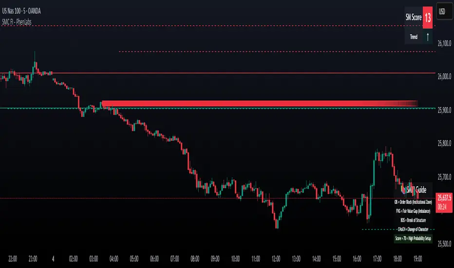
Aibuyzone Elliott Wave SuiteOverview
This study approximates Elliott-style wave structure using swing pivots. It labels primary waves (1–5), tracks subwaves (1–5) inside them, and plots future projection bands derived from the size of a recent primary leg. A small floating dashboard summarizes the current wave number, bias (bullish/bearish) based on the last leg, and a projection price range.
Note: This tool is educational. Wave detection is algorithmic and approximate; it does not identify textbook Elliott patterns or validate rule sets. Manage risk independently.
What it draws
Primary wave labels (1–5): Based on higher swing length pivots (major turns).
Subwave labels (1–5): Based on shorter swing length pivots (minor turns).
Zigzag connectors: Simple lines between the latest primary pivots for structure visualization.
Projection bands: Three dotted horizontal levels forward from the last primary pivot, using user-defined extension multipliers.
Floating dashboard:
Current Wave: Latest primary wave count (1–5).
Bias: “Bullish Leg” (last pivot was a low) or “Bearish Leg” (last pivot was a high), or “Unknown” if insufficient data.
Proj Range: Min–max of the three projection levels.
Key Inputs
Swing Structure
Primary Swing Length: Pivot left/right bars for major swings. Larger values = fewer, cleaner waves.
Subwave Swing Length: Pivot left/right bars for minor swings. Smaller values = more frequent subwave labels.
Max Saved Swing Points: Memory limit to prevent clutter.
Future Projections
Show Projection Levels: Toggle projection lines on/off.
Use Last Nth Leg For Size: Which recent primary leg to use for measuring projection distance (1 = most recent).
Extension 1 / 2 / 3: Multipliers applied to the measured leg (e.g., 1.0, 1.618, 2.0).
Style
Colors and text sizes for primary and subwave labels, and projection lines.
Dashboard
Show Dashboard: Toggle table on/off.
Dashboard Position: Top-Left / Top-Right / Bottom-Left / Bottom-Right.
How projections are computed
The script measures the price distance of a recent primary leg (from pivot A to pivot B).
If the last pivot is a low, projections extend upward; if the last pivot is a high, projections extend downward.
The three extension inputs (e.g., 1.0 / 1.618 / 2.0) are applied to that leg distance to create dotted forward levels.
The dashboard’s Proj Range displays the min–max of those three levels.
Using the study (suggested workflow)
Choose timeframe appropriate for your style (e.g., higher timeframes for cleaner structure; lower timeframes for detail).
Tune swing lengths:
Increase Primary Swing Length on noisy charts to stabilize wave counts.
Adjust Subwave Swing Length to reveal or simplify internal moves.
Read the dashboard:
Current Wave shows where the latest primary count sits (1–5).
Bias summarizes the direction of the last measured leg only; it is not a trend system.
Proj Range offers a coarse price band derived from your extensions.
Context check: Combine wave labeling with your own market context (trend, structure, volatility) before making decisions.
Risk management: Use your own stop/target methods. The projection lines are not signals.
Practical tips
Clutter control: If labels overlap on volatile symbols, try larger swing lengths or reduce label text sizes in Style.
Scaling: On very small tick sizes, increasing the internal label price offset can improve label readability.
Projection sensitivity: Changing Use Last Nth Leg can materially alter levels; confirm they match your intent.
Non-determinism across timeframes: Different timeframes and symbols will produce different pivot sequences and counts.
Limitations & important notes
Approximation: This does not enforce all Elliott rules (e.g., alternation, wave 4 overlap constraints, channeling). It only labels swings numerically.
Repainting of labels: Pivot-based waves confirm after enough bars have printed to the right of a high/low. Labels are placed when pivots confirm; they don’t predict pivots.
Not a signal generator: No entries/exits/alerts are included; add your own trade plan and risk controls.
Data sufficiency: Early bars or sparse data may show “Unknown” bias or “N/A” projections until adequate pivots exist.
Clean-chart publishing guidance (to stay compliant)
Use a chart that clearly shows this script’s outputs without unrelated indicators.
Keep the description educational. Avoid performance claims, guarantees, or language implying certainty.
Do not include links, promotions, prices, giveaways, contact details, or solicitations.
Disclose that labels and projections are algorithmic approximations and for educational use.
Risk disclosure
This script is for educational purposes only. It does not provide financial, investment, or trading advice and does not guarantee outcomes. Markets involve risk, including the potential loss of capital. Always do your own research and use independent judgment.

Lord Mathew ATSThe Smart Money Structure & Pattern Analyzer is a complete, all-in-one visual trading system that brings together every essential element of Smart Money Concepts (SMC), ICT methodology, and candlestick psychology into one powerful indicator.
It is designed to help traders instantly understand the market’s structure, liquidity flow, and potential turning points without switching tools or manually marking charts. Whether you trade forex, indices, crypto, or commodities, this indicator automatically identifies where institutional activity, imbalances, and price inefficiencies occur in real time.
With its advanced algorithm, it plots market structure shifts, equal highs and lows, liquidity zones, order blocks, fair value gaps (FVGs), and previous week and day levels (PWO, PWH, PWL, PWC, PDO, PDH, PDL, PDO). It also integrates a deep candlestick recognition engine that detects over ten classic and advanced candle formations including engulfing patterns, dojis, hammers, shooting stars, morning/evening stars, and spinning tops to provide precise confirmation at critical points of interest.
This indicator isn’t just a tool it’s a complete market map that helps traders visualize how institutional order flow and candlestick sentiment interact.
Core Features
📊 Market Structure Detection:
Automatically marks swing highs/lows, Break of Structure (BOS), and Change of Character (CHOCH) in real time.
💧 Liquidity Mapping:
Highlights equal highs/lows and liquidity grabs, showing where price is likely to target before a reversal or continuation.
🧱 Order Block Visualization:
Displays the last bullish or bearish candle before an impulsive displacement, acting as a potential institutional entry zone.
⚡ Fair Value Gap (FVG) Scanner:
Detects and highlights imbalances where price moved too fast, helping you identify high-probability retracement areas.
🕯️ Candlestick Pattern Recognition:
Recognizes key reversal and continuation patterns (engulfing, hammer, shooting star, doji, morning/evening star, etc.) in real time.
📅 Institutional Reference Points:
Plots previous week & day open (PWO, PDO), previous week & day high (PWH, PWH), previous week & day low (PWL, PDL), previous week & day close (PWC, PDC) and optionally previous day levels to help frame bias.
🎨 Customizable Design:
Toggle any feature, change colors, and set alerts when multiple Smart Money signals align for cleaner, faster decision-making.
How It Works
Add the indicator to your chart on any timeframe or market.
The algorithm automatically detects structure, liquidity, and imbalance zones.
Candlestick patterns are highlighted when they form near high-probability areas (like OBs or FVGs).
When confluence occurs such as a liquidity grab, FVG fill, and bullish engulfing candle—the indicator provides a visual signal zone for your confirmation-based entries.
You can refine your trades using higher-timeframe bias (HTF order flow) and lower-timeframe execution (LTF confirmation).
Best For
Traders using ICT, Smart Money Concepts, or price-action systems.
Intraday and swing traders looking for clear, data-driven chart structure.
Traders who want to simplify confluence analysis and focus on precision execution.
Why It Stands Out
Unlike standard candlestick or pattern scanners, this indicator merges institutional market logic with technical candle behavior, allowing traders to see where smart money might be entering or exiting positions.
It’s not about random signals it’s about context, structure, and confirmation.
Every feature in this indicator is built around the principle of liquidity engineering:
price creates liquidity, grabs it, and moves toward imbalance or order flow efficiency.
By merging that institutional logic with candlestick patterns, this tool gives traders an edge in recognizing not only where to trade but why price is reacting in that exact area.
Disclaimer
This indicator is intended for educational and analytical use. It does not provide financial advice or guaranteed trading results. Always backtest and manage your risk responsibly.
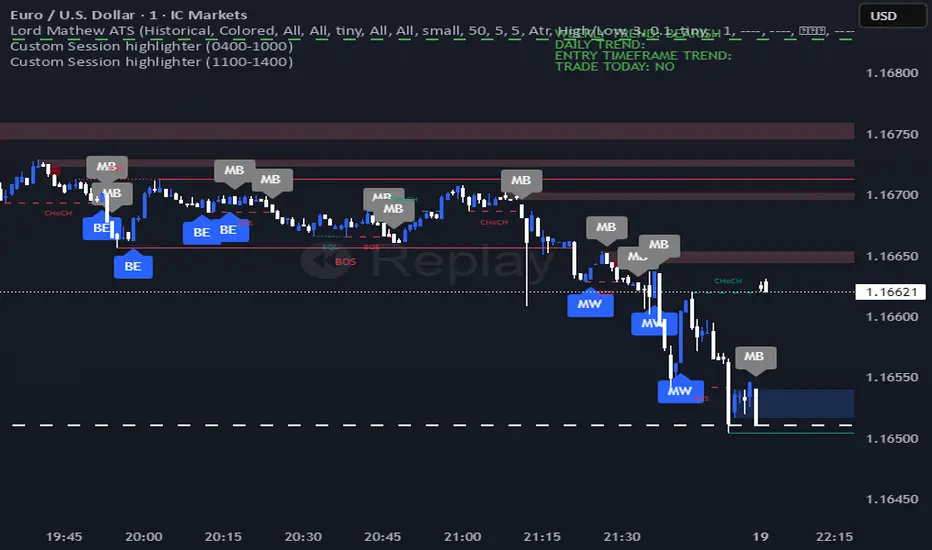
Smart Money Volume Tools | Lyro RSSmart Money Volume Tools | Lyro RS
Overview
The Smart Money Volume Tools (SMVT) is a multi-dimensional volume-based analysis suite designed to visualize the interplay between price action, moving averages, and smart money behavior.
By integrating dynamic moving averages, volume normalization, and multi-timeframe intelligence, SMVT helps traders identify when institutional (smart money) or retail participants are influencing price movements — all in a single, adaptive display.
Unlike traditional oscillators or trend tools, SMVT dynamically adjusts its sensitivity and thresholds based on volume z-scores and normalized momentum, revealing true intent behind price shifts rather than reacting to them.
🔹 Key Features
4 Core Analytical Modes:
Trail Mode – Identifies directional bias using dynamic volume-weighted trails based on adaptive ATR multipliers.
Volume Mode – Displays normalized volume strength vs. price trend, highlighting volume-driven expansions.
Smart Money Volume Mode – Detects institutional buying/selling spikes from lower timeframes using volume z-score outliers.
Retail Money Volume Mode – Contrasts retail-driven impulses to visualize crowd behavior and exhaustion points.
Dynamic Volume Normalization: Converts volume impulses into a 0–100 range using a sigmoid function for smoother interpretation.
Multi-Timeframe Intelligence: Automatically reads lower timeframe volume data to distinguish smart vs. retail activity.
Adaptive Color Systems: Multiple palette modes ( Classic , Mystic , Accented , Royal ) or full custom color control.
Signal Table Overlay: Built-in real-time module summary showing status for Trail , Volume , Smart Money , and Retail Money — right on your chart.
🔹 How It Works
Volume Strength Calculation:
Calculates relative volume strength using a moving average baseline, then normalizes the result via a sigmoid function — mapping activity into a clean 0–100 range.
Smart Money Detection:
Scans lower timeframe data for extreme volume z-scores ( z > 2 ) to pinpoint institutional accumulation or distribution zones.
Trail Logic:
Uses adaptive upper and lower trails based on ATR and volume intensity to track volatility-adjusted trend direction.
Color Logic:
Trail, candle, and fill colors change dynamically according to the active signal type and selected palette — making directional bias instantly visible.
🔹 Practical Use
Swing Confirmation (Trail Mode): Confirms sustained bullish or bearish momentum supported by volume, ideal for trailing positions and managing exits.
Volume Expansion (Volume Mode): Highlights key moments when institutional liquidity pushes price before visible breakout confirmation.
Smart vs. Retail Divergence: Identify conflicts between retail activity and smart money to detect exhaustion or reversal points early.
Table Overlay Utility: Instantly see all active signals across modules in one compact, on-chart interface.
🔹 Customization
Custom color palettes or manual bullish/bearish color selection.
Adjustable EMA lengths and Volume SMA period .
Selectable lower timeframe source for Smart Money analysis.
Flexible table position & size controls — choose between Top, Middle, Bottom and Tiny to Huge.
Switch freely between Trail , Volume , Smart Money , and Retail Money modes.
Credits
Thank you to @AlgoAlpha for the smart money and retail activity source code.
⚠️Disclaimer
This indicator is a tool for technical analysis and does not provide guaranteed results. It should be used in conjunction with other analysis methods and proper risk management practices. The creators of this indicator are not responsible for any financial decisions made based on its signals.
