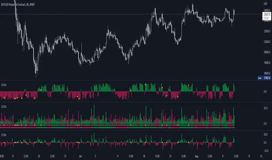
CCMA - Count Condition MA (560 Indicators In One) Do you like using moving averages?
Why do you think a pair of moving averages on a chart will help you?
What is the probability that once two moving averages have crossed, you will successfully enter the trade?
So why not use 100+ moving averages at once to increase the probability of a successful trade?
And all this can be seen in a single oscillator as a histogram!
I want to introduce you to a system that takes into account 560 moving averages movements. And that's just for a second, 560 potential indicators.
Specifically:
- 22 types of MA (EMA, SMA, RMA and others).
- 176 moving averages.
- 310 crossover checks.
- 252 checks of trend following.
The indicator makes the most of the opportunities provided by television. Therefore, it can take a long time to load it.
How does it work ?
In general, the indicator counts the number of fulfilled conditions.
It checks if MA #1 and MA #2 have crossed. If so, it adds +1 to the statistics. It also checks if price is above or below the moving average. There are a total of 560 such checks. (This is about the maximum the TV allowed me).
The default is 8 lengths of moving averages, I took the Fibonacci numbers thinking they were the optimal solution. You can take any of your favorites.
If the "Ratio MOD" feature is on. Then you can see how many MAs are showing signals to enter a long or short position.
You can also see the indication at the bottom as dots. They show which signals are longer/shorter. If the number of signals is the same, the dot will be yellow. The first line of dots counts the number of crossings. The second line counts the number of crossovers + checks whether the price is above or below the average slippage.
If the "Differ MOD" function is enabled. Then you can see the difference between long and short signals. With the same indication as in RATIO MOD.
If "Show all" is on, then the bar graph shows all 560 accounting options. If it is off, only the number of crossovers is displayed. (This does not apply to the display as points)
If the script shows an error, try to change the timeframe and go back. Or add it again.
You can also disable the histogram in the stats settings and leave only the points that help in determining the trend.
在脚本中搜索"averages"
Keltner Channel With User Selectable Moving AvgKeltner Channel with user options to calculate the moving average basis and envelopes from a variety of different moving averages.
The user selects their choice of moving average, and the envelopes automatically adjust. The user may select a MA that reacts faster to volatility or slower/smoother.
Added additional options to color the envelopes or basis based on the current trend and alternate candle colors for envelope touches. The script has a rainbow gradient by default based on RSI.
Options (generally from slower/smoother to faster/more responsive to volatility):
SMMA,
SMA,
Donchian, (Note: Selecting Donchian will just convert this indicator to a regular Donchian Channel)
Tillson T3,
EMA,
VWMA,
WMA,
EHMA,
ALMA,
LSMA,
HMA,
TEMA
Value Added:
Allows Keltner Channel to be calculated from a variety of moving averages other than EMA/SMA, including ones that are well liked by traders such as Tillson T3, ALMA, Hull MA, and TEMA.
Glossary:
The Hull Moving Average ( HMA ), developed by Alan Hull, is an extremely fast and smooth moving average . In fact, the HMA almost eliminates lag altogether and manages to improve smoothing at the same time.
The Exponential Hull Moving Average is similar to the standard Hull MA, but with superior smoothing. The standard Hull Moving Average is derived from the weighted moving average ( WMA ). As other moving average built from weighted moving averages it has a tendency to exaggerate price movement.
Weighted Moving Average: A Weighted Moving Average ( WMA ) is similar to the simple moving average ( SMA ), except the WMA adds significance to more recent data points.
Arnaud Legoux Moving Average: ALMA removes small price fluctuations and enhances the trend by applying a moving average twice, once from left to right, and once from right to left. At the end of this process the phase shift (price lag) commonly associated with moving averages is significantly reduced. Zero-phase digital filtering reduces noise in the signal. Conventional filtering reduces noise in the signal, but adds a delay.
Least Squares: Based on sum of least squares method to find a straight line that best fits data for the selected period. The end point of the line is plotted and the process is repeated on each succeeding period.
Triple EMA (TEMA) : The triple exponential moving average (TEMA) was designed to smooth price fluctuations, thereby making it easier to identify trends without the lag associated with traditional moving averages (MA). It does this by taking multiple exponential moving averages (EMA) of the original EMA and subtracting out some of the lag.
Running (SMoothed) Moving Average: A Modified Moving Average (MMA) (otherwise known as the Running Moving Average (RMA), or SMoothed Moving Average (SMMA)) is an indicator that shows the average value of a security's price over a period of time. It works very similar to the Exponential Moving Average, they are equivalent but for different periods (e.g., the MMA value for a 14-day period will be the same as EMA-value for a 27-days period).
Volume-Weighted Moving Average: The Volume-weighted Moving Average (VWMA) emphasizes volume by weighing prices based on the amount of trading activity in a given period of time. Users can set the length, the source and an offset. Prices with heavy trading activity get more weight than prices with light trading activity.
Tillson T3: The Tillson moving average a.k.a. the Tillson T3 indicator is one of the smoothest moving averages and is both composite and adaptive.

Adjustable MA & Alternating Extremities [LuxAlgo]Returns a moving average allowing the user to control the amount of lag as well as the amplitude of its overshoots thanks to a parametric kernel. The indicator displays alternating extremities and aims to provide potential points where price might reverse.
Due to user requests, we added the option to display the moving average as candles instead of a solid line.
Settings
Length: MA period, refers to the number of most recent data points to use for its calculation.
Mult: Multiplicative factor for each extremity.
As Smoothed Candles: Allows the user to show the MA as a series of candles instead of a solid line.
Show Alternating Extremities : Determines whether to display the alternating extremities or not.
Lag: Controls the amount of lag of the MA, with higher values returning a MA with more lag.
Overshoot: Controls the amplitude of the overshoots returned by the MA, with higher values increasing the amplitude of the overshoots.
Usage
Moving averages using parametric kernels allows users to have more control over characteristics such as lag or smoothness; this can greatly benefit the analyst. A moving average with reduced lag can be used as a leading moving average in a MA crossover system, while lag will benefit moving averages used as slow MA in a crossover system.
Increasing 'Lag' will increase smoothness while increasing 'overshoot' will reduce lag.
The following indicator puts more emphasis on its alternating extremities, an upper extremity will be shown once the high price crosses the upper extremity, while a low extremity will be shown once the low price crosses the lower extremity. These can be interpreted like extremities of a band indicator.
The MA using a length value of 200 with a multiplicative factor of 1.
In general, extremities will effectively return points where price might potentially bounce in ranging markets while closing prices under trending markets will often be found above an upper extremity and under a lower extremity.
Reducing the lag of the moving average allows the user to obtain a more timely estimate of the underlying trend in the price, with a better fit overall. This allows the user to obtain potentially pertinent extremities where price might reverse upon a break, even under trending markets.
In the above chart, the price initially breaks the upper extremity, however, we can observe that the upper extremity eventually reaches back the price, goes above it, provides a resistance, and effectively indicates a reversal.
Users can plot candles from the moving average, these are fairly similar to heikin-ashi candles in the sense that CandleOpen(t) ≠ CandleClose(t-1) , each point of the candle is calculated as follows for our indicator:
Open = Average between MA(t-1) and MA(t-2)
High = MA using the high price as input
Low = MA using the low price as input
Close = MA using the closing price as input
Details
Lag is defined as the effect of moving averages to reflect past price variations instead of new ones, lag can be observed by the user and is the main cause of false signals. Lag is proportional to the degree of filtering returned by the moving average.
Overshooting is a common effect encountered in non-lagging moving averages, and is defined as the tendency of a moving average to exceed a maximum level (or minimum level, which can be defined as undershooting )
MA and rolling maximum/minimum, both using a length of 50 bars. While we can think of lag as a cost of smoothness, we can think of overshooting as a cost for reduced lag on some occasions.
Explaining the kernel design behind our moving average requires understanding of the logic behind lag reduction in moving averages. This can prove to be complex for non informed users, but let's just focus on the simpler part; moving averages can be defined as a weighted sum between past prices and a set of coefficients (kernel).
MA(t) = b(0)C(t) + b(1)C(t-1) + b(2)C(t-2) + ... + b(n-1)C(t-n-1)
Where n is the period of the moving average. Lag is (non optimally) reduced by "underweighting" past prices - that is multiplying them by negative numbers.
The kernel used in our moving average is based on a modified sinewave. A weighted sum making use of a sinewave as a kernel would return an oscillator centered at 0. We can divide this sinewave by an increasing linear function in order to obtain a kernel allowing us to obtain a low lag moving average instead of a centered oscillator. This is the main idea in the design of the kernel used by our moving average.
The kernel equation of our moving average is:
sin(2πx^α)(1 - x^β)
With 1>x>0 , and where α controls the lag, while β controls the overshoot amplitude.
Using this equation we can obtain the following kernels:
Here only α is changed, while β is equal to 1. Values to the left would represent the coefficients for the most recent prices. Notice how the most significant coefficients are given to the oldest prices in the case where α increases.
Higher overshoot would require more negative values, this is controlled by β
Here only β is changed, while α is equal to 1. Notice how higher values return lower negative coefficients. This effectively increases the overshoots amplitude in our moving average. We can decrease α in order for these negative coefficients to underweight more recent values.
Using α = 0 allows us to simplify the kernel equation to:
1 - x^β
Using this kernel we can obtain more classical moving averages, this can be seen from the following results:
Using β = 1 allows us to obtain a linearly decreasing kernel (the one of a WMA), while increasing allows the kernel to converge toward a rectangular kernel (the one of SMA).

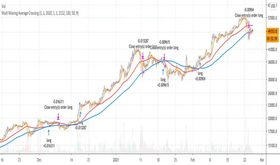
Multi Moving Average Crossing (by Coinrule)Moving Averages are among the most common trading indicators. They are straightforward to interpret and effective to use.
One of the limitations of using moving averages is they can provide buy and sell signals with a relatively high lag , making it very difficult to spot the lows and tops of the trend.
Moving averages calculated with a low number of periods like the MA9 (the average of the previous nine price periods) react very fast to price moves providing prompt signals. On the other side, more signals may end up with more false-signals and more trades in a loss.
On the contrary, moving averages calculated with a higher number of periods like the MA100 (which considers the previous one hundred price periods) give more reliable signals, but with a delay.
A system catching the crossing of the MA50 over the MA100 is a good compromise for successful long-term strategies. It provides, on average, reliable buy signals.
The Multi Moving Average Crossing Strategy tries to optimize the exit without waiting for the same opposite crossing (MA50 below MA100). It uses the MA9 crossing below the MA50, instead, to spot a better time for selling.
The setup is as follows.
BUY when the Moving Average 50 crosses above the Moving Average 100
SELL when the Moving Average 9 crosses below the Moving Average 50
The higher is the time frame to calculate the Moving Averages, the better is the overall performance of the strategy. The 4-hour (or 6-hour) time frame seems to be the best, even if it results in fewer trades. If you want to trade more still with good results, the 1-hour time is a good compromise.
Advantages of the strategy
This strategy seeks to catch those that are more likely relevant uptrends and close the trade relatively quickly. More trades mean more opportunities. This is especially effective if you run the strategy on all the available coins on the market, as you could do with Coinrule.
Generally, a Multi Moving Averages approach beats the classic crossing strategy involving only two Moving Averages. We backtested a sample of twenty trading pairs to assess the benefits empirically.
The results show that the Multi Moving Average Strategy
outperforms 13 out of 20 times
has 95% higher average return
has 67% higher median return
The strategy assumes each order to trade 30% of the available capital and opens a trade at a time. A trading fee of 0.1% is taken into account.
Red and Green Ignored Bar by Oliver VelezOn this occasion I present a script that detects Ignored Red Candles and Ignored Green Candles, basically it is a Price Action event that indicates a possible continuation of the current trend and gives the opportunity to climb it with a Very tight risk, before delving into detail I would like to leave this note:
Note: the detection of this event does not guarantee that the signal will be good, the trader must have the ability to determine its quality based on aspects such as trend, maturity, support / resistance levels, expansion / contraction of the market, risk / benefit, etc, if you do not have knowledge about this you should not use this indicator since using it without a robust trading plan and experience could cause you to partially or totally lose your money, if this is your case you should train before If you try to extract money from the market, this script was created to be another tool in your trading plan in order to configure the rules at your discretion, execute them consistently and have AUTOMATIC ALERTS when the event occurs, which is where I find more value because you can have many instruments waiting for the event to be generated, in the time frame you want and without having to observe the mer When the alert is generated, the Trader should evaluate the quality of the alert and define whether or not to execute it (higher timeframes, they can give you more time to execute the operation correctly).
Let's continue….
This event was created by Oliver Velez recognized trader / mentor of price action, the event has a very interesting particularity since it allows to take a position with a very limited risk in trend movements, this achieves favorable operations of good ratio and small losses when taking An adjusted risk, if the trade works, a good ratio is quickly achieved and we agree with a key point in the “Keep small losses and big profits” trading, this makes it easier to have a positive mathematical hope when your level of Success is not very high, so leave you in the field of profitability.
THE EVENT:
The event has a bullish configuration (Ignored Red Candle) and a bearish configuration (Ignored Green Candle), below I detail the “Hard” rules (later I explain why “Hard”):
1- Last 3 bars have to be GREEN-RED-GREEN (possible bullish configuration) or RED-GREEN-RED (possible bearish configuration), the first bar is called Control Bar, the second is called Ignored Bar and the third Signal Bar as shown in the following image:
2- Be in a trend determined by simple moving averages (Slow of 20 periods and Fast of 8 periods), as a general rule you can take the direction of MA20 but the Trader has to determine if there is a trend movement or not.
3- Control bar of good range, little tail and with a body greater than 55%.
4- Ignored bar preferably narrow range, little tail and that is located in the upper 1/3 of the control bar.
5- Signal bar cannot override the minimum of the ignored bar.
6- Activation / Confirmation of event by means of signal bar in overcoming the body of the ignored bar.
Some examples of ignored bars (with “Hard” and “Flexible” rules):
Features and configuration of the indicator:
To access the indicator settings, press the wheel next to the indicator name VVI_VRI "Configuration options".
- Operation mode (Filtering Type):
• Filtering Complete: all filters activated according to the configuration below.
• Without Filtering: all filters deactivated, all VRI / VVI are displayed without any selection criteria.
• Trend Filter only: shows only VRI / VVI that are in accordance with what is set in “Trend Settings”
- Configuration Moving Averages:
• See Slow Media: slow moving average display with direction detection and color change.
• See Fast Media: display of fast moving average with direction detection and color change.
• Type: possibility to choose the type of media: DEMA, EMA, HullMA, SMA, SSMA, SSMA, TEMA, TMA, VWMA, WMA, ZEMA)
• Period: number of previous bars.
• Source: possibility to choose the type of source, open, close, high, low, hl2 hlc3, ohlc4.
• Reaction: this configuration affects the color change before a change of direction, 1 being an immediate reaction and higher values, a more delayed reaction obtaining les false "changes of direction", a value of 3 filters the direction quite well.
- Trend Configuration
• Uptrend Condition P / VRI: possibility to select any of these conditions:
o Bullish MA direction
o Quick bullish MA direction
o Slow and fast bullish MA direction
o Price higher than slow MA
o Price higher than fast MA
o Price higher than slow and fast MA
o Price higher than slow MA and bullish direction
o Price higher than fast MA and bullish direction
o Price higher than slow, fast MA and bullish direction
o No condition
• Condition P / VVI bear trend: possibility of selecting any of these conditions:
o Slow bearish MA direction
o Fast bearish MA direction
o Slow and fast bearish MA direction
o Price less than slow MA
o Price less than fast MA
o Price less than slow and fast MA
o Price lower than slow MA and bearish direction
o Price less than fast MA and bearish direction
o Price less than slow, fast MA and bearish direction
o No condition
- Control bar configuration
• Minimum body percentage%: possibility to select what body percentage the bar must have.
• Paint control bar: when selected, paint the control bar.
• See control bar label: when selected, a label with the legend BC is plotted.
- Configuration bar ignored
• Above X% of the control bar: possibility to select above what percentage of the control bar the ignored bar must be located.
• Paint ignored bar: when selected, paint the ignored bar.
- Signal bar configuration
• You cannot override the minimum of the ignored bar: when selected, the condition is added that the signal bar cannot override the minimum of the ignored bar.
• Paint signal bar: when selected, paint the signal bar.
• See arrow: when selected it shows the direction arrow of the possible movement.
• See bear and arrow: when selected it shows bear and arrow label
• See bull and arrow: when selected it shows bull and arrow label
The following image shows the ignored bar and painted signal:
- Take profit / loss
The profit / loss taking varies depending on the trader and its risk / monetary plan, the proposal is a recommendation based on the nature of the event that is to have a small risk unit (stop below the minimum of the ignored bar), look for objectives in ratios greater than 2: 1 and eliminate the risk in 1: 1 by taking the stop to BE, all parameters are configurable and are the following:
• See recommended stop loss and take profit: trace the levels of Stop, BE, TP1 and TP2, as well as their prices to know them quickly based on the assumed risk
• To: select which event you want to draw the SL and TP (VRI, VVI)
• Extend stop loss line x bars: allows extending the stop line by x number of bars
• Extend take profit line x bars: allows extending the stop line by x number of bars
• Ratio to move to break even: allows you to select the minimum ratio to move stop to break even (default 1: 1)
• Take profit 1 ratio: allows you to select the ratio for take profit 1 (default 2: 1)
• Take profit 2 ratio: allows you to select the ratio for take profit 2 (default 4: 1)
- Alerts
• It is possible to configure the following alerts:
-VRI DETECTED
-VVI DETECTED
-VRI / VVI DETECTED
Final Notes:
- The term hard rules refers to the fact that an event is sought with the rules detailed above to obtain a high quality event but this brings 2 situations to consider, less
number of events and events that are generated in a strong impulse may be leaked, a very large control bar followed by an ignored narrow body away from moving averages, despite having a good chance of continuing, taking a stop very tight in a strong impulse you can touch it by the simple fact of the own volatility at that time.
- The setting of the parameters “Minimum body percentage% (control bar)”, “Above x% of the control bar (bar ignored)” and “Cannot override the minimum of the ignored bar” can bring large Benefits in terms of number of events and that can also be of high quality, feel free to find the best configuration for your instrument to operate.
- It is recommended to look for trending events, near moving averages and at an early stage of it.
- The display of several nearby VRIs or VVIs in an advanced trend may indicate a depletion of it.
- The alerts can be worked in 2 ways: at the closing of the candle (confirms event but the risk unit may be larger or smaller) or immediately the body of the ignored bar is exceeded, in case you are operating from the mobile and miss many events because of the short time I recommend that you operate in a superior time frame to have more time.
- The indicator is configured with “flexible” rules to have more events, but without any important criteria, each trader has to look for the best configuration that suits his instrument.
- It is recommended to partially close the operation based on the ratio and always keep a part of the position to apply manual trailing stop and try to maximize profits.
The code is open feel free to use and modify it, a mention in credits is appreciated.
If you liked this SCRIPT THUMB UP!
Greetings to all, I wish you much green!

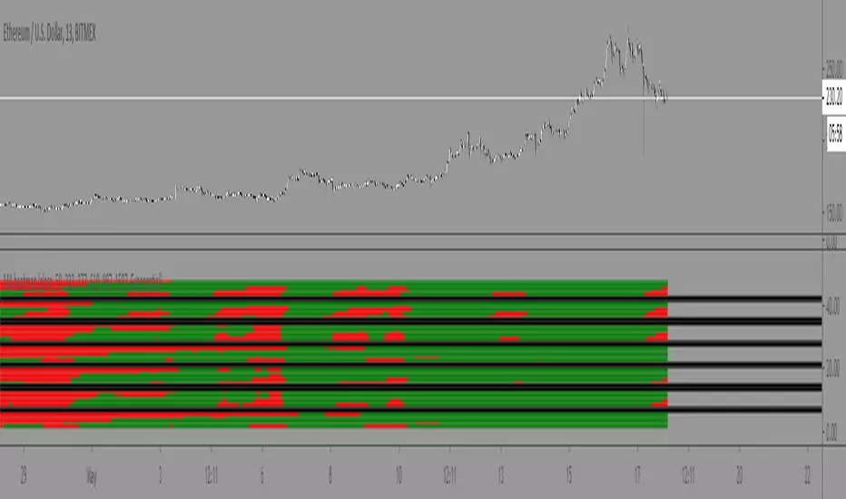
Moving Average Heatmap Visualization7 different types of moving averages (5 different lengths of each) compared to a base moving average. Base moving average can be configured to be a slew of different types of moving averages (credit to @mortdiggiddy for the code) and have a custom length.
Red = base moving average is over other moving average (bearish)
Green = base moving average is under other moving average (bullish)
lengths for the different MAs are just fibonacci numbers due to lack of creativity.
First 5 moving averages are Simple moving average the next 5 are Exponential moving averages and after that it is weighted moving averages, volume weighted moving average (VWAP), Exponential volume weighted moving average (thanks again @mortdiggiddy ), hull moving averages and lastly zero lag moving averages.
The indicator might lag your chart out a bit so be ready for that.
Have fun!
[blackcat] L1 Simple Dual Channel Breakout█ OVERVIEW
The script " L1 Simple Dual Channel Breakout" is an indicator designed to plot dual channel breakout bands and their long-term EMAs on a chart. It calculates short-term and long-term moving averages and deviations to establish upper, lower, and middle bands, which traders can use to identify potential breakout opportunities.
█ LOGICAL FRAMEWORK
Structure:
The script is structured into several main sections:
• Input Parameters: The script does not explicitly define input parameters for the user to adjust, but it uses default values for short_term_length (5) and long_term_length (181).
• Calculations: The calculate_dual_channel_breakout function performs the core calculations, including the blast condition, typical price, short-term and long-term moving averages, and dynamic moving averages.
• Plotting: The script plots the short-term bands (upper, lower, and middle) and their long-term EMAs. It also plots conditional line breaks when the short-term bands cross the long-term EMAs.
Flow of Data and Logic:
1 — The script starts by defining the calculate_dual_channel_breakout function.
2 — Inside the function, it calculates various moving averages and deviations based on the input prices and lengths.
3 — The function returns the calculated bands and EMAs.
4 — The script then calls this function with predefined lengths and plots the resulting bands and EMAs on the chart.
5 — Conditional plots are added to highlight breakouts when the short-term bands cross the long-term EMAs.
█ CUSTOM FUNCTIONS
The script defines one custom function:
• calculate_dual_channel_breakout(close_price, high_price, low_price, short_term_length, long_term_length): This function calculates the short-term and long-term bands and EMAs. It takes five parameters: close_price, high_price, low_price, short_term_length, and long_term_length. It returns an array containing the upper band, lower band, middle band, long-term upper EMA, long-term lower EMA, and long-term middle EMA.
█ KEY POINTS AND TECHNIQUES
• Typical Price Calculation: The script uses a modified typical price calculation (2 * close_price + high_price + low_price) / 4 instead of the standard (high_price + low_price + close_price) / 3.
• Short-term and Long-term Bands: The script calculates short-term bands using a simple moving average (SMA) of the typical price and long-term bands using a relative moving average (RMA) of the close price.
• Conditional Plotting: The script uses conditional plotting to highlight breakouts when the short-term bands cross the long-term EMAs, enhancing visual identification of trading signals.
• EMA for Long-term Trends: The use of Exponential Moving Averages (EMAs) for long-term bands helps in smoothing out short-term fluctuations and focusing on long-term trends.
█ EXTENDED KNOWLEDGE AND APPLICATIONS
• Modifications: Users can add input parameters to allow customization of short_term_length and long_term_length, making the indicator more flexible.
• Enhancements: The script could be extended to include alerts for breakout conditions, providing traders with real-time notifications.
• Alternative Bands: Users might experiment with different types of moving averages (e.g., WMA, HMA) for the short-term and long-term bands to see if they yield better results.
• Additional Indicators: Combining this indicator with other technical indicators (e.g., RSI, MACD) could provide a more comprehensive trading strategy.
• Backtesting: Users can backtest the strategy using Pine Script's strategy functions to evaluate its performance over historical data.

UDC - Local TrendsUDC - Local Trends Indicator
Overview:
The UDC - Local Trends Indicator combines multiple moving averages to provide a clear visualization of both local and high timeframe (HTF) trends. This indicator helps traders make informed decisions by highlighting key moving averages and trend zones, making it easier to determine whether the current trend is likely to continue or reverse.
Features:
Local Trend Zone: Displays the range between the 13 and 34 EMAs, with an average line in the middle. This zone is plotted close to the price candles, offering a clear visual guide for the immediate trend on the timeframe you’re viewing.
Usage: Observe the strength of the local trend within this zone. Breaks from this zone may indicate potential moves toward the 200 moving averages, providing early signals for trend continuation or potential reversals.
Current Trend Indicators:
Tracks the broader trend using the 200 EMA and 200 SMA on the active timeframe. Choose a timeframe where these trend lines hold significance and use them alongside support and resistance for precise entries and exits.
Cross-Timeframe Trend Reference:
On all sub-daily timeframes, the daily 200 moving average is overlaid, ensuring this essential trend line is visible even on shorter timeframes, like 4H, where reclaims or rejections of the daily 200 can signal strong trading setups.
The weekly 50 moving average, a critical HTF trend line, is also displayed consistently, guiding higher timeframe swing trade setups.
Trading Strategy:
Local Timeframe Trading:
Monitor the 200 moving averages in your active timeframe to identify bounces or breakdowns. If the local trend zone (13-34 EMA range) is lost, expect a possible pullback to the 200 moving averages, offering a chance for re-entry or confirmation of trend reversal.
High Timeframe Trading (HTF):
For swing trades, observe the daily 200 and weekly 50 moving averages. Reclaiming these lines often triggers long setups, while losing them may signal further downside until they’re regained.
This indicator offers a powerful combination of localized trend tracking and high timeframe support, enabling traders to align their entries with both immediate and overarching market

MTF EHMA & HMA Insights [FibonacciFlux]MTF EHMA & HMA Insights
Overview
The Multi-Timeframe EHMA, HMA, and Midline with Fill script is a powerful technical analysis tool designed for traders seeking to enhance their market insights and decision-making processes. By integrating two advanced moving averages—Exponential Hull Moving Average (EHMA) and Hull Moving Average (HMA)—along with a dynamic midline, this indicator provides a comprehensive view of market trends across multiple timeframes.
Key Features
1. Dual Moving Averages
- Exponential Hull Moving Average (EHMA) :
- Offers a rapid response to price changes, making it particularly useful for identifying short-term trends.
- Utilizes a unique calculation method that reduces lag, allowing traders to react quickly to market movements.
- Hull Moving Average (HMA) :
- Known for its smoothness and ability to filter out noise, the HMA presents a clear picture of the underlying trend.
- The HMA is specifically designed to achieve a balance between responsiveness and smoothness, enabling traders to make informed decisions.
2. Midline Calculation
- Dynamic Midline (m) :
- The midline is calculated as the average of EHMA and HMA, providing a neutral reference point for evaluating price movements.
- It visually represents market sentiment; a rising midline suggests bullish conditions, while a declining midline indicates bearish trends.
3. Visual Components
- Fill Areas :
- Color-coded fills between the EHMA and HMA enhance visual clarity by indicating the relative position of these moving averages.
- The fill color dynamically changes based on the relationship between the two averages (green for EHMA below HMA and red for EHMA above HMA), allowing traders to quickly assess market conditions.
4. Signal Generation and Alerts
- Buy/Sell Signals :
- The indicator generates buy signals when the midline crosses above its previous value, indicating a potential upward trend.
- Conversely, sell signals are triggered when the midline crosses below its previous value, suggesting a possible downward movement.
- Alert Conditions :
- Built-in alerts notify traders in real-time when significant changes occur, allowing them to act swiftly on potential trading opportunities.
- Customizable alert messages ensure traders receive relevant information tailored to their strategies.
Technical Details
Input Parameters
- Timeframe Settings :
- Traders can customize the timeframes for both EHMA and HMA, enabling them to adapt the indicator to different trading styles and market conditions.
- Length Settings :
- Adjustable lengths for both moving averages impact their sensitivity, allowing traders to optimize their performance based on volatility and market dynamics.
Plotting and Visualization
- Plotting :
- The script plots the EHMA, HMA, and midline directly on the chart for easy visualization.
- Signal labels (BUY and SELL) are displayed prominently, helping traders to identify potential entry and exit points without ambiguity.
Benefits
1. Clarity and Insight
- The combination of EHMA, HMA, and midline provides a clear and concise visual representation of market trends, aiding traders in making informed decisions.
2. Flexibility
- Customizable parameters allow traders to tailor the indicator to their specific needs, making it suitable for various market conditions and trading styles.
3. Efficiency
- Real-time alerts and visual signals minimize response times, enabling traders to capitalize on opportunities as they arise.
4. Enhanced Trading Conditions
- When utilizing the Fibonacci number 144 on a daily chart, the indicator facilitates optimal trading conditions:
- "The entry was made before the bubble began, using 144 as the Fibonacci variable."
- "The exit occurred right before the bubble burst, or alternatively, a short position was initiated."
- "When the next bubble started, a long entry was made again."
- "Despite some lag, the position was exited and a long entry was made."
- "The exit or short entry took place at the second double top peak."
- "A short position was already established before the double top formation occurred."
- On a 4-hour chart, traders can effectively set stop losses at HMA levels, achieving a risk-reward ratio between 4 and 8.
- Additionally, analyzing the 15-minute chart with a multi-timeframe approach allows for more precise entry points.
Conclusion
The Multi-Timeframe EHMA, HMA, and Midline with Fill script is a robust tool for traders looking to enhance their technical analysis capabilities. By combining multiple moving averages with a dynamic midline and alert system, this indicator offers a comprehensive approach to understanding market trends. Its flexibility, clarity, and efficiency make it an invaluable asset for both novice and experienced traders alike.
Important Note
As with any trading tool, it is crucial to conduct thorough analysis and risk management when using this indicator. Past performance does not guarantee future results, and traders should always be prepared for potential market fluctuations.

MA Optimizer Simplified [CHE]Introduction:
The MA Optimizer Simplified is a powerful tool for traders and analysts who want to compare and optimize various moving averages (MA). This tool is specifically designed to identify the best or worst performers among a variety of moving averages based on their cumulative performance.
Features and Benefits:
1. Versatility:
- Supports multiple types of moving averages, including:
- Simple Moving Average (SMA): A basic MA calculated by averaging the closing prices over a specified period.
- Exponential Moving Average (EMA): Gives more weight to recent prices, making it more responsive to new information.
- Weighted Moving Average (WMA): Assigns more weight to recent data, but in a linear fashion.
- Volume-Weighted Moving Average (VWMA): Averages prices based on volume, giving more importance to periods with higher trading volume.
- Hull Moving Average (HMA): Designed to reduce lag while improving smoothness.
- Smoothed Moving Average (SMMA or RMA): Averages prices over a longer period, providing a smoother line.
- Bollinger Bands: Uses SMA as a basis and adds upper and lower bands based on standard deviations.
- T3: A smoother and less lagging MA that reduces market noise.
- Allows users to easily switch between MA types and test different periods.
2. Performance Evaluation:
- Calculates the cumulative performance of up to ten different MAs.
- Automatically identifies the best or worst performer based on user selection (Best or Worst).
3. Crossover Detection:
- Detects crossovers of prices and MAs to measure performance.
- Provides clear visual signals when the price crosses a moving average.
4. Visual Representation:
- Plots the best MA indicator on the chart, dynamically changing its color based on price movement relative to the MA.
- Table functionality to display the performance of each MA, including the length and achieved performance in percentage.
5. Customizable Settings:
- Customizable settings for table size and position as well as colors for better visualization and user-friendliness.
- Flexibility in selecting the number of candles that must be above or below the MA before a signal is triggered.
Special Features:
1. T3 Indicator:
- The T3 indicator provides a smoother representation and reduces market noise, leading to more precise signals.
2. Crossover and Crossunder Logic:
- The script includes advanced logic for detecting crossover and crossunder events to identify accurate entry points.
3. Dynamic Color Change:
- The best MA indicator changes color based on the number of candles above or below the MA, helping to quickly recognize market sentiment.
4. Comprehensive Performance Analysis:
- The calculation of cumulative performance for each MA allows for detailed analysis and helps identify the most effective trading strategies.
Conclusion:
The MA Optimizer Simplified is an essential tool for any trader looking to analyze and optimize the performance of various moving averages. With its versatile features and user-friendly settings, it offers a comprehensive and efficient solution for technical analysis.
Best regards, Chervolino

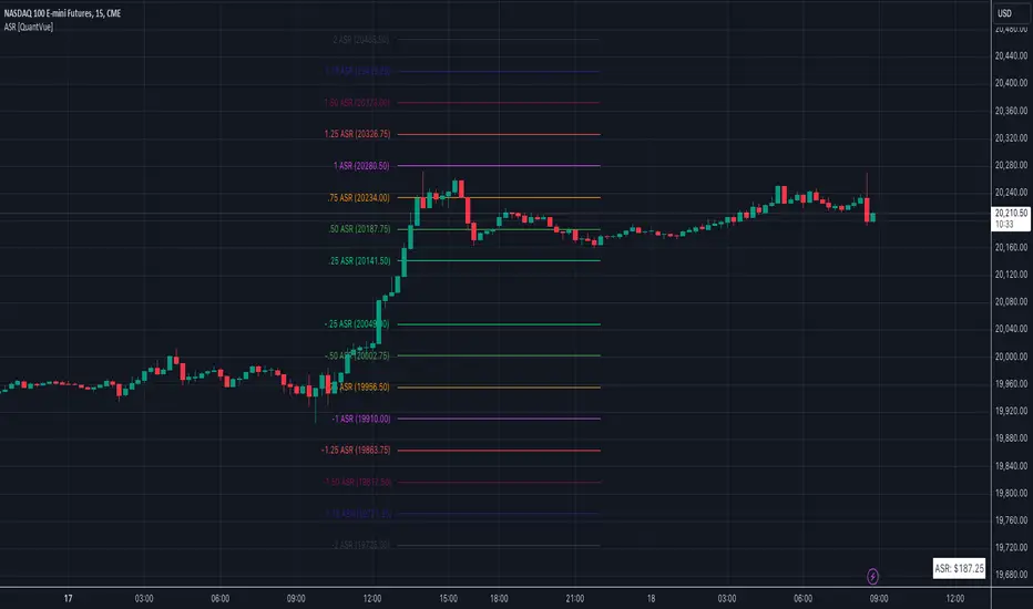
Average Session Range [QuantVue]The Average Session Range or ASR is a tool designed to find the average range of a user defined session over a user defined lookback period.
Not only is this indicator is useful for understanding volatility and price movement tendencies within sessions, but it also plots dynamic support and resistance levels based on the ASR.
The average session range is calculated over a specific period (default 14 sessions) by averaging the range (high - low) for each session.
Knowing what the ASR is allows the user to determine if current price action is normal or abnormal.
When a new session begins, potential support and resistance levels are calculated by breaking the ASR into quartiles which are then added and subtracted from the sessions opening price.
The indicator also shows an ASR label so traders can know what the ASR is in terms of dollars.
Session Time Configuration:
The indicator allows users to define the session time, with default timing set from 13:00 to 22:00.
ASR Calculation:
The ASR is calculated over a specified period (default 14 sessions) by averaging the range (high - low) of each session.
Various levels based on the ASR are computed: 0.25 ASR, 0.5 ASR, 0.75 ASR, 1 ASR, 1.25 ASR, 1.5 ASR, 1.75 ASR, and 2 ASR.
Visual Representation:
The indicator plots lines on the chart representing different ASR levels.
Customize the visibility, color, width, and style (Solid, Dashed, Dotted) of these lines for better visualization.
Labels for these lines can also be displayed, with customizable positions and text properties.
Give this indicator a BOOST and COMMENT your thoughts!
We hope you enjoy.
Cheers!
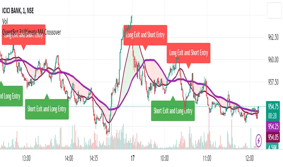
QuantBot 3:Ultimate MA CrossoverTHIS IS A SAMPLE CODE TO AUTOMATE WITH QUANTBOT
The moving average strategy is a popular and widely used technique in financial analysis and trading. It involves the calculation and analysis of moving averages, which are mathematical indicators that smooth out price data over a specified period. This strategy is primarily applied in the context of stock trading, but it can be used for other financial instruments as well.
The concept behind the moving average strategy is to identify trends and potential entry or exit points in the market. By calculating and analyzing moving averages of different timeframes, traders aim to capture the overall direction of the price movement and filter out short-term fluctuations or noise.
To implement the moving average strategy, a trader typically selects two or more moving averages with different periods. The most common combinations include the 50-day and 200-day moving averages. The shorter-term moving average is considered more reactive to price changes, while the longer-term moving average provides a smoother trend line. When the shorter-term moving average crosses above the longer-term moving average, it generates a buy signal, indicating a potential upward trend. Conversely, when the shorter-term moving average crosses below the longer-term moving average, it generates a sell signal, indicating a potential downward trend.
Traders can use various variations of the moving average strategy based on their trading objectives and risk tolerance. For instance, some traders may prefer to use exponential moving averages (EMAs) instead of simple moving averages (SMAs) to give more weight to recent price data. Others may incorporate additional indicators or filters to confirm signals or avoid false signals.
One of the strengths of the moving average strategy is its simplicity and ease of interpretation. It provides a clear visual representation of the trend direction and potential entry or exit points. However, it's important to note that the moving average strategy is a lagging indicator, meaning that it relies on past price data. Therefore, it may not always accurately predict future market movements or capture sudden reversals.
Like any trading strategy, the moving average strategy is not foolproof and carries risks. It is crucial for traders to conduct thorough analysis, consider other relevant factors, and manage their risk through proper position sizing and risk management techniques. Additionally, it's important to adapt the strategy to specific market conditions and combine it with other complementary strategies or indicators for improved decision-making.
Overall, the moving average strategy serves as a valuable tool for traders to identify and follow trends in financial markets, aiding in the analysis of price movements and potential trading opportunities.
Goertzel Cycle Composite Wave [Loxx]As the financial markets become increasingly complex and data-driven, traders and analysts must leverage powerful tools to gain insights and make informed decisions. One such tool is the Goertzel Cycle Composite Wave indicator, a sophisticated technical analysis indicator that helps identify cyclical patterns in financial data. This powerful tool is capable of detecting cyclical patterns in financial data, helping traders to make better predictions and optimize their trading strategies. With its unique combination of mathematical algorithms and advanced charting capabilities, this indicator has the potential to revolutionize the way we approach financial modeling and trading.
*** To decrease the load time of this indicator, only XX many bars back will render to the chart. You can control this value with the setting "Number of Bars to Render". This doesn't have anything to do with repainting or the indicator being endpointed***
█ Brief Overview of the Goertzel Cycle Composite Wave
The Goertzel Cycle Composite Wave is a sophisticated technical analysis tool that utilizes the Goertzel algorithm to analyze and visualize cyclical components within a financial time series. By identifying these cycles and their characteristics, the indicator aims to provide valuable insights into the market's underlying price movements, which could potentially be used for making informed trading decisions.
The Goertzel Cycle Composite Wave is considered a non-repainting and endpointed indicator. This means that once a value has been calculated for a specific bar, that value will not change in subsequent bars, and the indicator is designed to have a clear start and end point. This is an important characteristic for indicators used in technical analysis, as it allows traders to make informed decisions based on historical data without the risk of hindsight bias or future changes in the indicator's values. This means traders can use this indicator trading purposes.
The repainting version of this indicator with forecasting, cycle selection/elimination options, and data output table can be found here:
Goertzel Browser
The primary purpose of this indicator is to:
1. Detect and analyze the dominant cycles present in the price data.
2. Reconstruct and visualize the composite wave based on the detected cycles.
To achieve this, the indicator performs several tasks:
1. Detrending the price data: The indicator preprocesses the price data using various detrending techniques, such as Hodrick-Prescott filters, zero-lag moving averages, and linear regression, to remove the underlying trend and focus on the cyclical components.
2. Applying the Goertzel algorithm: The indicator applies the Goertzel algorithm to the detrended price data, identifying the dominant cycles and their characteristics, such as amplitude, phase, and cycle strength.
3. Constructing the composite wave: The indicator reconstructs the composite wave by combining the detected cycles, either by using a user-defined list of cycles or by selecting the top N cycles based on their amplitude or cycle strength.
4. Visualizing the composite wave: The indicator plots the composite wave, using solid lines for the cycles. The color of the lines indicates whether the wave is increasing or decreasing.
This indicator is a powerful tool that employs the Goertzel algorithm to analyze and visualize the cyclical components within a financial time series. By providing insights into the underlying price movements, the indicator aims to assist traders in making more informed decisions.
█ What is the Goertzel Algorithm?
The Goertzel algorithm, named after Gerald Goertzel, is a digital signal processing technique that is used to efficiently compute individual terms of the Discrete Fourier Transform (DFT). It was first introduced in 1958, and since then, it has found various applications in the fields of engineering, mathematics, and physics.
The Goertzel algorithm is primarily used to detect specific frequency components within a digital signal, making it particularly useful in applications where only a few frequency components are of interest. The algorithm is computationally efficient, as it requires fewer calculations than the Fast Fourier Transform (FFT) when detecting a small number of frequency components. This efficiency makes the Goertzel algorithm a popular choice in applications such as:
1. Telecommunications: The Goertzel algorithm is used for decoding Dual-Tone Multi-Frequency (DTMF) signals, which are the tones generated when pressing buttons on a telephone keypad. By identifying specific frequency components, the algorithm can accurately determine which button has been pressed.
2. Audio processing: The algorithm can be used to detect specific pitches or harmonics in an audio signal, making it useful in applications like pitch detection and tuning musical instruments.
3. Vibration analysis: In the field of mechanical engineering, the Goertzel algorithm can be applied to analyze vibrations in rotating machinery, helping to identify faulty components or signs of wear.
4. Power system analysis: The algorithm can be used to measure harmonic content in power systems, allowing engineers to assess power quality and detect potential issues.
The Goertzel algorithm is used in these applications because it offers several advantages over other methods, such as the FFT:
1. Computational efficiency: The Goertzel algorithm requires fewer calculations when detecting a small number of frequency components, making it more computationally efficient than the FFT in these cases.
2. Real-time analysis: The algorithm can be implemented in a streaming fashion, allowing for real-time analysis of signals, which is crucial in applications like telecommunications and audio processing.
3. Memory efficiency: The Goertzel algorithm requires less memory than the FFT, as it only computes the frequency components of interest.
4. Precision: The algorithm is less susceptible to numerical errors compared to the FFT, ensuring more accurate results in applications where precision is essential.
The Goertzel algorithm is an efficient digital signal processing technique that is primarily used to detect specific frequency components within a signal. Its computational efficiency, real-time capabilities, and precision make it an attractive choice for various applications, including telecommunications, audio processing, vibration analysis, and power system analysis. The algorithm has been widely adopted since its introduction in 1958 and continues to be an essential tool in the fields of engineering, mathematics, and physics.
█ Goertzel Algorithm in Quantitative Finance: In-Depth Analysis and Applications
The Goertzel algorithm, initially designed for signal processing in telecommunications, has gained significant traction in the financial industry due to its efficient frequency detection capabilities. In quantitative finance, the Goertzel algorithm has been utilized for uncovering hidden market cycles, developing data-driven trading strategies, and optimizing risk management. This section delves deeper into the applications of the Goertzel algorithm in finance, particularly within the context of quantitative trading and analysis.
Unveiling Hidden Market Cycles:
Market cycles are prevalent in financial markets and arise from various factors, such as economic conditions, investor psychology, and market participant behavior. The Goertzel algorithm's ability to detect and isolate specific frequencies in price data helps trader analysts identify hidden market cycles that may otherwise go unnoticed. By examining the amplitude, phase, and periodicity of each cycle, traders can better understand the underlying market structure and dynamics, enabling them to develop more informed and effective trading strategies.
Developing Quantitative Trading Strategies:
The Goertzel algorithm's versatility allows traders to incorporate its insights into a wide range of trading strategies. By identifying the dominant market cycles in a financial instrument's price data, traders can create data-driven strategies that capitalize on the cyclical nature of markets.
For instance, a trader may develop a mean-reversion strategy that takes advantage of the identified cycles. By establishing positions when the price deviates from the predicted cycle, the trader can profit from the subsequent reversion to the cycle's mean. Similarly, a momentum-based strategy could be designed to exploit the persistence of a dominant cycle by entering positions that align with the cycle's direction.
Enhancing Risk Management:
The Goertzel algorithm plays a vital role in risk management for quantitative strategies. By analyzing the cyclical components of a financial instrument's price data, traders can gain insights into the potential risks associated with their trading strategies.
By monitoring the amplitude and phase of dominant cycles, a trader can detect changes in market dynamics that may pose risks to their positions. For example, a sudden increase in amplitude may indicate heightened volatility, prompting the trader to adjust position sizing or employ hedging techniques to protect their portfolio. Additionally, changes in phase alignment could signal a potential shift in market sentiment, necessitating adjustments to the trading strategy.
Expanding Quantitative Toolkits:
Traders can augment the Goertzel algorithm's insights by combining it with other quantitative techniques, creating a more comprehensive and sophisticated analysis framework. For example, machine learning algorithms, such as neural networks or support vector machines, could be trained on features extracted from the Goertzel algorithm to predict future price movements more accurately.
Furthermore, the Goertzel algorithm can be integrated with other technical analysis tools, such as moving averages or oscillators, to enhance their effectiveness. By applying these tools to the identified cycles, traders can generate more robust and reliable trading signals.
The Goertzel algorithm offers invaluable benefits to quantitative finance practitioners by uncovering hidden market cycles, aiding in the development of data-driven trading strategies, and improving risk management. By leveraging the insights provided by the Goertzel algorithm and integrating it with other quantitative techniques, traders can gain a deeper understanding of market dynamics and devise more effective trading strategies.
█ Indicator Inputs
src: This is the source data for the analysis, typically the closing price of the financial instrument.
detrendornot: This input determines the method used for detrending the source data. Detrending is the process of removing the underlying trend from the data to focus on the cyclical components.
The available options are:
hpsmthdt: Detrend using Hodrick-Prescott filter centered moving average.
zlagsmthdt: Detrend using zero-lag moving average centered moving average.
logZlagRegression: Detrend using logarithmic zero-lag linear regression.
hpsmth: Detrend using Hodrick-Prescott filter.
zlagsmth: Detrend using zero-lag moving average.
DT_HPper1 and DT_HPper2: These inputs define the period range for the Hodrick-Prescott filter centered moving average when detrendornot is set to hpsmthdt.
DT_ZLper1 and DT_ZLper2: These inputs define the period range for the zero-lag moving average centered moving average when detrendornot is set to zlagsmthdt.
DT_RegZLsmoothPer: This input defines the period for the zero-lag moving average used in logarithmic zero-lag linear regression when detrendornot is set to logZlagRegression.
HPsmoothPer: This input defines the period for the Hodrick-Prescott filter when detrendornot is set to hpsmth.
ZLMAsmoothPer: This input defines the period for the zero-lag moving average when detrendornot is set to zlagsmth.
MaxPer: This input sets the maximum period for the Goertzel algorithm to search for cycles.
squaredAmp: This boolean input determines whether the amplitude should be squared in the Goertzel algorithm.
useAddition: This boolean input determines whether the Goertzel algorithm should use addition for combining the cycles.
useCosine: This boolean input determines whether the Goertzel algorithm should use cosine waves instead of sine waves.
UseCycleStrength: This boolean input determines whether the Goertzel algorithm should compute the cycle strength, which is a normalized measure of the cycle's amplitude.
WindowSizePast: These inputs define the window size for the composite wave.
FilterBartels: This boolean input determines whether Bartel's test should be applied to filter out non-significant cycles.
BartNoCycles: This input sets the number of cycles to be used in Bartel's test.
BartSmoothPer: This input sets the period for the moving average used in Bartel's test.
BartSigLimit: This input sets the significance limit for Bartel's test, below which cycles are considered insignificant.
SortBartels: This boolean input determines whether the cycles should be sorted by their Bartel's test results.
StartAtCycle: This input determines the starting index for selecting the top N cycles when UseCycleList is set to false. This allows you to skip a certain number of cycles from the top before selecting the desired number of cycles.
UseTopCycles: This input sets the number of top cycles to use for constructing the composite wave when UseCycleList is set to false. The cycles are ranked based on their amplitudes or cycle strengths, depending on the UseCycleStrength input.
SubtractNoise: This boolean input determines whether to subtract the noise (remaining cycles) from the composite wave. If set to true, the composite wave will only include the top N cycles specified by UseTopCycles.
█ Exploring Auxiliary Functions
The following functions demonstrate advanced techniques for analyzing financial markets, including zero-lag moving averages, Bartels probability, detrending, and Hodrick-Prescott filtering. This section examines each function in detail, explaining their purpose, methodology, and applications in finance. We will examine how each function contributes to the overall performance and effectiveness of the indicator and how they work together to create a powerful analytical tool.
Zero-Lag Moving Average:
The zero-lag moving average function is designed to minimize the lag typically associated with moving averages. This is achieved through a two-step weighted linear regression process that emphasizes more recent data points. The function calculates a linearly weighted moving average (LWMA) on the input data and then applies another LWMA on the result. By doing this, the function creates a moving average that closely follows the price action, reducing the lag and improving the responsiveness of the indicator.
The zero-lag moving average function is used in the indicator to provide a responsive, low-lag smoothing of the input data. This function helps reduce the noise and fluctuations in the data, making it easier to identify and analyze underlying trends and patterns. By minimizing the lag associated with traditional moving averages, this function allows the indicator to react more quickly to changes in market conditions, providing timely signals and improving the overall effectiveness of the indicator.
Bartels Probability:
The Bartels probability function calculates the probability of a given cycle being significant in a time series. It uses a mathematical test called the Bartels test to assess the significance of cycles detected in the data. The function calculates coefficients for each detected cycle and computes an average amplitude and an expected amplitude. By comparing these values, the Bartels probability is derived, indicating the likelihood of a cycle's significance. This information can help in identifying and analyzing dominant cycles in financial markets.
The Bartels probability function is incorporated into the indicator to assess the significance of detected cycles in the input data. By calculating the Bartels probability for each cycle, the indicator can prioritize the most significant cycles and focus on the market dynamics that are most relevant to the current trading environment. This function enhances the indicator's ability to identify dominant market cycles, improving its predictive power and aiding in the development of effective trading strategies.
Detrend Logarithmic Zero-Lag Regression:
The detrend logarithmic zero-lag regression function is used for detrending data while minimizing lag. It combines a zero-lag moving average with a linear regression detrending method. The function first calculates the zero-lag moving average of the logarithm of input data and then applies a linear regression to remove the trend. By detrending the data, the function isolates the cyclical components, making it easier to analyze and interpret the underlying market dynamics.
The detrend logarithmic zero-lag regression function is used in the indicator to isolate the cyclical components of the input data. By detrending the data, the function enables the indicator to focus on the cyclical movements in the market, making it easier to analyze and interpret market dynamics. This function is essential for identifying cyclical patterns and understanding the interactions between different market cycles, which can inform trading decisions and enhance overall market understanding.
Bartels Cycle Significance Test:
The Bartels cycle significance test is a function that combines the Bartels probability function and the detrend logarithmic zero-lag regression function to assess the significance of detected cycles. The function calculates the Bartels probability for each cycle and stores the results in an array. By analyzing the probability values, traders and analysts can identify the most significant cycles in the data, which can be used to develop trading strategies and improve market understanding.
The Bartels cycle significance test function is integrated into the indicator to provide a comprehensive analysis of the significance of detected cycles. By combining the Bartels probability function and the detrend logarithmic zero-lag regression function, this test evaluates the significance of each cycle and stores the results in an array. The indicator can then use this information to prioritize the most significant cycles and focus on the most relevant market dynamics. This function enhances the indicator's ability to identify and analyze dominant market cycles, providing valuable insights for trading and market analysis.
Hodrick-Prescott Filter:
The Hodrick-Prescott filter is a popular technique used to separate the trend and cyclical components of a time series. The function applies a smoothing parameter to the input data and calculates a smoothed series using a two-sided filter. This smoothed series represents the trend component, which can be subtracted from the original data to obtain the cyclical component. The Hodrick-Prescott filter is commonly used in economics and finance to analyze economic data and financial market trends.
The Hodrick-Prescott filter is incorporated into the indicator to separate the trend and cyclical components of the input data. By applying the filter to the data, the indicator can isolate the trend component, which can be used to analyze long-term market trends and inform trading decisions. Additionally, the cyclical component can be used to identify shorter-term market dynamics and provide insights into potential trading opportunities. The inclusion of the Hodrick-Prescott filter adds another layer of analysis to the indicator, making it more versatile and comprehensive.
Detrending Options: Detrend Centered Moving Average:
The detrend centered moving average function provides different detrending methods, including the Hodrick-Prescott filter and the zero-lag moving average, based on the selected detrending method. The function calculates two sets of smoothed values using the chosen method and subtracts one set from the other to obtain a detrended series. By offering multiple detrending options, this function allows traders and analysts to select the most appropriate method for their specific needs and preferences.
The detrend centered moving average function is integrated into the indicator to provide users with multiple detrending options, including the Hodrick-Prescott filter and the zero-lag moving average. By offering multiple detrending methods, the indicator allows users to customize the analysis to their specific needs and preferences, enhancing the indicator's overall utility and adaptability. This function ensures that the indicator can cater to a wide range of trading styles and objectives, making it a valuable tool for a diverse group of market participants.
The auxiliary functions functions discussed in this section demonstrate the power and versatility of mathematical techniques in analyzing financial markets. By understanding and implementing these functions, traders and analysts can gain valuable insights into market dynamics, improve their trading strategies, and make more informed decisions. The combination of zero-lag moving averages, Bartels probability, detrending methods, and the Hodrick-Prescott filter provides a comprehensive toolkit for analyzing and interpreting financial data. The integration of advanced functions in a financial indicator creates a powerful and versatile analytical tool that can provide valuable insights into financial markets. By combining the zero-lag moving average,
█ In-Depth Analysis of the Goertzel Cycle Composite Wave Code
The Goertzel Cycle Composite Wave code is an implementation of the Goertzel Algorithm, an efficient technique to perform spectral analysis on a signal. The code is designed to detect and analyze dominant cycles within a given financial market data set. This section will provide an extremely detailed explanation of the code, its structure, functions, and intended purpose.
Function signature and input parameters:
The Goertzel Cycle Composite Wave function accepts numerous input parameters for customization, including source data (src), the current bar (forBar), sample size (samplesize), period (per), squared amplitude flag (squaredAmp), addition flag (useAddition), cosine flag (useCosine), cycle strength flag (UseCycleStrength), past sizes (WindowSizePast), Bartels filter flag (FilterBartels), Bartels-related parameters (BartNoCycles, BartSmoothPer, BartSigLimit), sorting flag (SortBartels), and output buffers (goeWorkPast, cyclebuffer, amplitudebuffer, phasebuffer, cycleBartelsBuffer).
Initializing variables and arrays:
The code initializes several float arrays (goeWork1, goeWork2, goeWork3, goeWork4) with the same length as twice the period (2 * per). These arrays store intermediate results during the execution of the algorithm.
Preprocessing input data:
The input data (src) undergoes preprocessing to remove linear trends. This step enhances the algorithm's ability to focus on cyclical components in the data. The linear trend is calculated by finding the slope between the first and last values of the input data within the sample.
Iterative calculation of Goertzel coefficients:
The core of the Goertzel Cycle Composite Wave algorithm lies in the iterative calculation of Goertzel coefficients for each frequency bin. These coefficients represent the spectral content of the input data at different frequencies. The code iterates through the range of frequencies, calculating the Goertzel coefficients using a nested loop structure.
Cycle strength computation:
The code calculates the cycle strength based on the Goertzel coefficients. This is an optional step, controlled by the UseCycleStrength flag. The cycle strength provides information on the relative influence of each cycle on the data per bar, considering both amplitude and cycle length. The algorithm computes the cycle strength either by squaring the amplitude (controlled by squaredAmp flag) or using the actual amplitude values.
Phase calculation:
The Goertzel Cycle Composite Wave code computes the phase of each cycle, which represents the position of the cycle within the input data. The phase is calculated using the arctangent function (math.atan) based on the ratio of the imaginary and real components of the Goertzel coefficients.
Peak detection and cycle extraction:
The algorithm performs peak detection on the computed amplitudes or cycle strengths to identify dominant cycles. It stores the detected cycles in the cyclebuffer array, along with their corresponding amplitudes and phases in the amplitudebuffer and phasebuffer arrays, respectively.
Sorting cycles by amplitude or cycle strength:
The code sorts the detected cycles based on their amplitude or cycle strength in descending order. This allows the algorithm to prioritize cycles with the most significant impact on the input data.
Bartels cycle significance test:
If the FilterBartels flag is set, the code performs a Bartels cycle significance test on the detected cycles. This test determines the statistical significance of each cycle and filters out the insignificant cycles. The significant cycles are stored in the cycleBartelsBuffer array. If the SortBartels flag is set, the code sorts the significant cycles based on their Bartels significance values.
Waveform calculation:
The Goertzel Cycle Composite Wave code calculates the waveform of the significant cycles for specified time windows. The windows are defined by the WindowSizePast parameters, respectively. The algorithm uses either cosine or sine functions (controlled by the useCosine flag) to calculate the waveforms for each cycle. The useAddition flag determines whether the waveforms should be added or subtracted.
Storing waveforms in a matrix:
The calculated waveforms for the cycle is stored in the matrix - goeWorkPast. This matrix holds the waveforms for the specified time windows. Each row in the matrix represents a time window position, and each column corresponds to a cycle.
Returning the number of cycles:
The Goertzel Cycle Composite Wave function returns the total number of detected cycles (number_of_cycles) after processing the input data. This information can be used to further analyze the results or to visualize the detected cycles.
The Goertzel Cycle Composite Wave code is a comprehensive implementation of the Goertzel Algorithm, specifically designed for detecting and analyzing dominant cycles within financial market data. The code offers a high level of customization, allowing users to fine-tune the algorithm based on their specific needs. The Goertzel Cycle Composite Wave's combination of preprocessing, iterative calculations, cycle extraction, sorting, significance testing, and waveform calculation makes it a powerful tool for understanding cyclical components in financial data.
█ Generating and Visualizing Composite Waveform
The indicator calculates and visualizes the composite waveform for specified time windows based on the detected cycles. Here's a detailed explanation of this process:
Updating WindowSizePast:
The WindowSizePast is updated to ensure they are at least twice the MaxPer (maximum period).
Initializing matrices and arrays:
The matrix goeWorkPast is initialized to store the Goertzel results for specified time windows. Multiple arrays are also initialized to store cycle, amplitude, phase, and Bartels information.
Preparing the source data (srcVal) array:
The source data is copied into an array, srcVal, and detrended using one of the selected methods (hpsmthdt, zlagsmthdt, logZlagRegression, hpsmth, or zlagsmth).
Goertzel function call:
The Goertzel function is called to analyze the detrended source data and extract cycle information. The output, number_of_cycles, contains the number of detected cycles.
Initializing arrays for waveforms:
The goertzel array is initialized to store the endpoint Goertzel.
Calculating composite waveform (goertzel array):
The composite waveform is calculated by summing the selected cycles (either from the user-defined cycle list or the top cycles) and optionally subtracting the noise component.
Drawing composite waveform (pvlines):
The composite waveform is drawn on the chart using solid lines. The color of the lines is determined by the direction of the waveform (green for upward, red for downward).
To summarize, this indicator generates a composite waveform based on the detected cycles in the financial data. It calculates the composite waveforms and visualizes them on the chart using colored lines.
█ Enhancing the Goertzel Algorithm-Based Script for Financial Modeling and Trading
The Goertzel algorithm-based script for detecting dominant cycles in financial data is a powerful tool for financial modeling and trading. It provides valuable insights into the past behavior of these cycles. However, as with any algorithm, there is always room for improvement. This section discusses potential enhancements to the existing script to make it even more robust and versatile for financial modeling, general trading, advanced trading, and high-frequency finance trading.
Enhancements for Financial Modeling
Data preprocessing: One way to improve the script's performance for financial modeling is to introduce more advanced data preprocessing techniques. This could include removing outliers, handling missing data, and normalizing the data to ensure consistent and accurate results.
Additional detrending and smoothing methods: Incorporating more sophisticated detrending and smoothing techniques, such as wavelet transform or empirical mode decomposition, can help improve the script's ability to accurately identify cycles and trends in the data.
Machine learning integration: Integrating machine learning techniques, such as artificial neural networks or support vector machines, can help enhance the script's predictive capabilities, leading to more accurate financial models.
Enhancements for General and Advanced Trading
Customizable indicator integration: Allowing users to integrate their own technical indicators can help improve the script's effectiveness for both general and advanced trading. By enabling the combination of the dominant cycle information with other technical analysis tools, traders can develop more comprehensive trading strategies.
Risk management and position sizing: Incorporating risk management and position sizing functionality into the script can help traders better manage their trades and control potential losses. This can be achieved by calculating the optimal position size based on the user's risk tolerance and account size.
Multi-timeframe analysis: Enhancing the script to perform multi-timeframe analysis can provide traders with a more holistic view of market trends and cycles. By identifying dominant cycles on different timeframes, traders can gain insights into the potential confluence of cycles and make better-informed trading decisions.
Enhancements for High-Frequency Finance Trading
Algorithm optimization: To ensure the script's suitability for high-frequency finance trading, optimizing the algorithm for faster execution is crucial. This can be achieved by employing efficient data structures and refining the calculation methods to minimize computational complexity.
Real-time data streaming: Integrating real-time data streaming capabilities into the script can help high-frequency traders react to market changes more quickly. By continuously updating the cycle information based on real-time market data, traders can adapt their strategies accordingly and capitalize on short-term market fluctuations.
Order execution and trade management: To fully leverage the script's capabilities for high-frequency trading, implementing functionality for automated order execution and trade management is essential. This can include features such as stop-loss and take-profit orders, trailing stops, and automated trade exit strategies.
While the existing Goertzel algorithm-based script is a valuable tool for detecting dominant cycles in financial data, there are several potential enhancements that can make it even more powerful for financial modeling, general trading, advanced trading, and high-frequency finance trading. By incorporating these improvements, the script can become a more versatile and effective tool for traders and financial analysts alike.
█ Understanding the Limitations of the Goertzel Algorithm
While the Goertzel algorithm-based script for detecting dominant cycles in financial data provides valuable insights, it is important to be aware of its limitations and drawbacks. Some of the key drawbacks of this indicator are:
Lagging nature:
As with many other technical indicators, the Goertzel algorithm-based script can suffer from lagging effects, meaning that it may not immediately react to real-time market changes. This lag can lead to late entries and exits, potentially resulting in reduced profitability or increased losses.
Parameter sensitivity:
The performance of the script can be sensitive to the chosen parameters, such as the detrending methods, smoothing techniques, and cycle detection settings. Improper parameter selection may lead to inaccurate cycle detection or increased false signals, which can negatively impact trading performance.
Complexity:
The Goertzel algorithm itself is relatively complex, making it difficult for novice traders or those unfamiliar with the concept of cycle analysis to fully understand and effectively utilize the script. This complexity can also make it challenging to optimize the script for specific trading styles or market conditions.
Overfitting risk:
As with any data-driven approach, there is a risk of overfitting when using the Goertzel algorithm-based script. Overfitting occurs when a model becomes too specific to the historical data it was trained on, leading to poor performance on new, unseen data. This can result in misleading signals and reduced trading performance.
Limited applicability:
The Goertzel algorithm-based script may not be suitable for all markets, trading styles, or timeframes. Its effectiveness in detecting cycles may be limited in certain market conditions, such as during periods of extreme volatility or low liquidity.
While the Goertzel algorithm-based script offers valuable insights into dominant cycles in financial data, it is essential to consider its drawbacks and limitations when incorporating it into a trading strategy. Traders should always use the script in conjunction with other technical and fundamental analysis tools, as well as proper risk management, to make well-informed trading decisions.
█ Interpreting Results
The Goertzel Cycle Composite Wave indicator can be interpreted by analyzing the plotted lines. The indicator plots two lines: composite waves. The composite wave represents the composite wave of the price data.
The composite wave line displays a solid line, with green indicating a bullish trend and red indicating a bearish trend.
Interpreting the Goertzel Cycle Composite Wave indicator involves identifying the trend of the composite wave lines and matching them with the corresponding bullish or bearish color.
█ Conclusion
The Goertzel Cycle Composite Wave indicator is a powerful tool for identifying and analyzing cyclical patterns in financial markets. Its ability to detect multiple cycles of varying frequencies and strengths make it a valuable addition to any trader's technical analysis toolkit. However, it is important to keep in mind that the Goertzel Cycle Composite Wave indicator should be used in conjunction with other technical analysis tools and fundamental analysis to achieve the best results. With continued refinement and development, the Goertzel Cycle Composite Wave indicator has the potential to become a highly effective tool for financial modeling, general trading, advanced trading, and high-frequency finance trading. Its accuracy and versatility make it a promising candidate for further research and development.
█ Footnotes
What is the Bartels Test for Cycle Significance?
The Bartels Cycle Significance Test is a statistical method that determines whether the peaks and troughs of a time series are statistically significant. The test is named after its inventor, George Bartels, who developed it in the mid-20th century.
The Bartels test is designed to analyze the cyclical components of a time series, which can help traders and analysts identify trends and cycles in financial markets. The test calculates a Bartels statistic, which measures the degree of non-randomness or autocorrelation in the time series.
The Bartels statistic is calculated by first splitting the time series into two halves and calculating the range of the peaks and troughs in each half. The test then compares these ranges using a t-test, which measures the significance of the difference between the two ranges.
If the Bartels statistic is greater than a critical value, it indicates that the peaks and troughs in the time series are non-random and that there is a significant cyclical component to the data. Conversely, if the Bartels statistic is less than the critical value, it suggests that the peaks and troughs are random and that there is no significant cyclical component.
The Bartels Cycle Significance Test is particularly useful in financial analysis because it can help traders and analysts identify significant cycles in asset prices, which can in turn inform investment decisions. However, it is important to note that the test is not perfect and can produce false signals in certain situations, particularly in noisy or volatile markets. Therefore, it is always recommended to use the test in conjunction with other technical and fundamental indicators to confirm trends and cycles.
Deep-dive into the Hodrick-Prescott Fitler
The Hodrick-Prescott (HP) filter is a statistical tool used in economics and finance to separate a time series into two components: a trend component and a cyclical component. It is a powerful tool for identifying long-term trends in economic and financial data and is widely used by economists, central banks, and financial institutions around the world.
The HP filter was first introduced in the 1990s by economists Robert Hodrick and Edward Prescott. It is a simple, two-parameter filter that separates a time series into a trend component and a cyclical component. The trend component represents the long-term behavior of the data, while the cyclical component captures the shorter-term fluctuations around the trend.
The HP filter works by minimizing the following objective function:
Minimize: (Sum of Squared Deviations) + λ (Sum of Squared Second Differences)
Where:
1. The first term represents the deviation of the data from the trend.
2. The second term represents the smoothness of the trend.
3. λ is a smoothing parameter that determines the degree of smoothness of the trend.
The smoothing parameter λ is typically set to a value between 100 and 1600, depending on the frequency of the data. Higher values of λ lead to a smoother trend, while lower values lead to a more volatile trend.
The HP filter has several advantages over other smoothing techniques. It is a non-parametric method, meaning that it does not make any assumptions about the underlying distribution of the data. It also allows for easy comparison of trends across different time series and can be used with data of any frequency.
However, the HP filter also has some limitations. It assumes that the trend is a smooth function, which may not be the case in some situations. It can also be sensitive to changes in the smoothing parameter λ, which may result in different trends for the same data. Additionally, the filter may produce unrealistic trends for very short time series.
Despite these limitations, the HP filter remains a valuable tool for analyzing economic and financial data. It is widely used by central banks and financial institutions to monitor long-term trends in the economy, and it can be used to identify turning points in the business cycle. The filter can also be used to analyze asset prices, exchange rates, and other financial variables.
The Hodrick-Prescott filter is a powerful tool for analyzing economic and financial data. It separates a time series into a trend component and a cyclical component, allowing for easy identification of long-term trends and turning points in the business cycle. While it has some limitations, it remains a valuable tool for economists, central banks, and financial institutions around the world.

Goertzel Browser [Loxx]As the financial markets become increasingly complex and data-driven, traders and analysts must leverage powerful tools to gain insights and make informed decisions. One such tool is the Goertzel Browser indicator, a sophisticated technical analysis indicator that helps identify cyclical patterns in financial data. This powerful tool is capable of detecting cyclical patterns in financial data, helping traders to make better predictions and optimize their trading strategies. With its unique combination of mathematical algorithms and advanced charting capabilities, this indicator has the potential to revolutionize the way we approach financial modeling and trading.
█ Brief Overview of the Goertzel Browser
The Goertzel Browser is a sophisticated technical analysis tool that utilizes the Goertzel algorithm to analyze and visualize cyclical components within a financial time series. By identifying these cycles and their characteristics, the indicator aims to provide valuable insights into the market's underlying price movements, which could potentially be used for making informed trading decisions.
The primary purpose of this indicator is to:
1. Detect and analyze the dominant cycles present in the price data.
2. Reconstruct and visualize the composite wave based on the detected cycles.
3. Project the composite wave into the future, providing a potential roadmap for upcoming price movements.
To achieve this, the indicator performs several tasks:
1. Detrending the price data: The indicator preprocesses the price data using various detrending techniques, such as Hodrick-Prescott filters, zero-lag moving averages, and linear regression, to remove the underlying trend and focus on the cyclical components.
2. Applying the Goertzel algorithm: The indicator applies the Goertzel algorithm to the detrended price data, identifying the dominant cycles and their characteristics, such as amplitude, phase, and cycle strength.
3. Constructing the composite wave: The indicator reconstructs the composite wave by combining the detected cycles, either by using a user-defined list of cycles or by selecting the top N cycles based on their amplitude or cycle strength.
4. Visualizing the composite wave: The indicator plots the composite wave, using solid lines for the past and dotted lines for the future projections. The color of the lines indicates whether the wave is increasing or decreasing.
5. Displaying cycle information: The indicator provides a table that displays detailed information about the detected cycles, including their rank, period, Bartel's test results, amplitude, and phase.
This indicator is a powerful tool that employs the Goertzel algorithm to analyze and visualize the cyclical components within a financial time series. By providing insights into the underlying price movements and their potential future trajectory, the indicator aims to assist traders in making more informed decisions.
█ What is the Goertzel Algorithm?
The Goertzel algorithm, named after Gerald Goertzel, is a digital signal processing technique that is used to efficiently compute individual terms of the Discrete Fourier Transform (DFT). It was first introduced in 1958, and since then, it has found various applications in the fields of engineering, mathematics, and physics.
The Goertzel algorithm is primarily used to detect specific frequency components within a digital signal, making it particularly useful in applications where only a few frequency components are of interest. The algorithm is computationally efficient, as it requires fewer calculations than the Fast Fourier Transform (FFT) when detecting a small number of frequency components. This efficiency makes the Goertzel algorithm a popular choice in applications such as:
1. Telecommunications: The Goertzel algorithm is used for decoding Dual-Tone Multi-Frequency (DTMF) signals, which are the tones generated when pressing buttons on a telephone keypad. By identifying specific frequency components, the algorithm can accurately determine which button has been pressed.
2. Audio processing: The algorithm can be used to detect specific pitches or harmonics in an audio signal, making it useful in applications like pitch detection and tuning musical instruments.
3. Vibration analysis: In the field of mechanical engineering, the Goertzel algorithm can be applied to analyze vibrations in rotating machinery, helping to identify faulty components or signs of wear.
4. Power system analysis: The algorithm can be used to measure harmonic content in power systems, allowing engineers to assess power quality and detect potential issues.
The Goertzel algorithm is used in these applications because it offers several advantages over other methods, such as the FFT:
1. Computational efficiency: The Goertzel algorithm requires fewer calculations when detecting a small number of frequency components, making it more computationally efficient than the FFT in these cases.
2. Real-time analysis: The algorithm can be implemented in a streaming fashion, allowing for real-time analysis of signals, which is crucial in applications like telecommunications and audio processing.
3. Memory efficiency: The Goertzel algorithm requires less memory than the FFT, as it only computes the frequency components of interest.
4. Precision: The algorithm is less susceptible to numerical errors compared to the FFT, ensuring more accurate results in applications where precision is essential.
The Goertzel algorithm is an efficient digital signal processing technique that is primarily used to detect specific frequency components within a signal. Its computational efficiency, real-time capabilities, and precision make it an attractive choice for various applications, including telecommunications, audio processing, vibration analysis, and power system analysis. The algorithm has been widely adopted since its introduction in 1958 and continues to be an essential tool in the fields of engineering, mathematics, and physics.
█ Goertzel Algorithm in Quantitative Finance: In-Depth Analysis and Applications
The Goertzel algorithm, initially designed for signal processing in telecommunications, has gained significant traction in the financial industry due to its efficient frequency detection capabilities. In quantitative finance, the Goertzel algorithm has been utilized for uncovering hidden market cycles, developing data-driven trading strategies, and optimizing risk management. This section delves deeper into the applications of the Goertzel algorithm in finance, particularly within the context of quantitative trading and analysis.
Unveiling Hidden Market Cycles:
Market cycles are prevalent in financial markets and arise from various factors, such as economic conditions, investor psychology, and market participant behavior. The Goertzel algorithm's ability to detect and isolate specific frequencies in price data helps trader analysts identify hidden market cycles that may otherwise go unnoticed. By examining the amplitude, phase, and periodicity of each cycle, traders can better understand the underlying market structure and dynamics, enabling them to develop more informed and effective trading strategies.
Developing Quantitative Trading Strategies:
The Goertzel algorithm's versatility allows traders to incorporate its insights into a wide range of trading strategies. By identifying the dominant market cycles in a financial instrument's price data, traders can create data-driven strategies that capitalize on the cyclical nature of markets.
For instance, a trader may develop a mean-reversion strategy that takes advantage of the identified cycles. By establishing positions when the price deviates from the predicted cycle, the trader can profit from the subsequent reversion to the cycle's mean. Similarly, a momentum-based strategy could be designed to exploit the persistence of a dominant cycle by entering positions that align with the cycle's direction.
Enhancing Risk Management:
The Goertzel algorithm plays a vital role in risk management for quantitative strategies. By analyzing the cyclical components of a financial instrument's price data, traders can gain insights into the potential risks associated with their trading strategies.
By monitoring the amplitude and phase of dominant cycles, a trader can detect changes in market dynamics that may pose risks to their positions. For example, a sudden increase in amplitude may indicate heightened volatility, prompting the trader to adjust position sizing or employ hedging techniques to protect their portfolio. Additionally, changes in phase alignment could signal a potential shift in market sentiment, necessitating adjustments to the trading strategy.
Expanding Quantitative Toolkits:
Traders can augment the Goertzel algorithm's insights by combining it with other quantitative techniques, creating a more comprehensive and sophisticated analysis framework. For example, machine learning algorithms, such as neural networks or support vector machines, could be trained on features extracted from the Goertzel algorithm to predict future price movements more accurately.
Furthermore, the Goertzel algorithm can be integrated with other technical analysis tools, such as moving averages or oscillators, to enhance their effectiveness. By applying these tools to the identified cycles, traders can generate more robust and reliable trading signals.
The Goertzel algorithm offers invaluable benefits to quantitative finance practitioners by uncovering hidden market cycles, aiding in the development of data-driven trading strategies, and improving risk management. By leveraging the insights provided by the Goertzel algorithm and integrating it with other quantitative techniques, traders can gain a deeper understanding of market dynamics and devise more effective trading strategies.
█ Indicator Inputs
src: This is the source data for the analysis, typically the closing price of the financial instrument.
detrendornot: This input determines the method used for detrending the source data. Detrending is the process of removing the underlying trend from the data to focus on the cyclical components.
The available options are:
hpsmthdt: Detrend using Hodrick-Prescott filter centered moving average.
zlagsmthdt: Detrend using zero-lag moving average centered moving average.
logZlagRegression: Detrend using logarithmic zero-lag linear regression.
hpsmth: Detrend using Hodrick-Prescott filter.
zlagsmth: Detrend using zero-lag moving average.
DT_HPper1 and DT_HPper2: These inputs define the period range for the Hodrick-Prescott filter centered moving average when detrendornot is set to hpsmthdt.
DT_ZLper1 and DT_ZLper2: These inputs define the period range for the zero-lag moving average centered moving average when detrendornot is set to zlagsmthdt.
DT_RegZLsmoothPer: This input defines the period for the zero-lag moving average used in logarithmic zero-lag linear regression when detrendornot is set to logZlagRegression.
HPsmoothPer: This input defines the period for the Hodrick-Prescott filter when detrendornot is set to hpsmth.
ZLMAsmoothPer: This input defines the period for the zero-lag moving average when detrendornot is set to zlagsmth.
MaxPer: This input sets the maximum period for the Goertzel algorithm to search for cycles.
squaredAmp: This boolean input determines whether the amplitude should be squared in the Goertzel algorithm.
useAddition: This boolean input determines whether the Goertzel algorithm should use addition for combining the cycles.
useCosine: This boolean input determines whether the Goertzel algorithm should use cosine waves instead of sine waves.
UseCycleStrength: This boolean input determines whether the Goertzel algorithm should compute the cycle strength, which is a normalized measure of the cycle's amplitude.
WindowSizePast and WindowSizeFuture: These inputs define the window size for past and future projections of the composite wave.
FilterBartels: This boolean input determines whether Bartel's test should be applied to filter out non-significant cycles.
BartNoCycles: This input sets the number of cycles to be used in Bartel's test.
BartSmoothPer: This input sets the period for the moving average used in Bartel's test.
BartSigLimit: This input sets the significance limit for Bartel's test, below which cycles are considered insignificant.
SortBartels: This boolean input determines whether the cycles should be sorted by their Bartel's test results.
UseCycleList: This boolean input determines whether a user-defined list of cycles should be used for constructing the composite wave. If set to false, the top N cycles will be used.
Cycle1, Cycle2, Cycle3, Cycle4, and Cycle5: These inputs define the user-defined list of cycles when 'UseCycleList' is set to true. If using a user-defined list, each of these inputs represents the period of a specific cycle to include in the composite wave.
StartAtCycle: This input determines the starting index for selecting the top N cycles when UseCycleList is set to false. This allows you to skip a certain number of cycles from the top before selecting the desired number of cycles.
UseTopCycles: This input sets the number of top cycles to use for constructing the composite wave when UseCycleList is set to false. The cycles are ranked based on their amplitudes or cycle strengths, depending on the UseCycleStrength input.
SubtractNoise: This boolean input determines whether to subtract the noise (remaining cycles) from the composite wave. If set to true, the composite wave will only include the top N cycles specified by UseTopCycles.
█ Exploring Auxiliary Functions
The following functions demonstrate advanced techniques for analyzing financial markets, including zero-lag moving averages, Bartels probability, detrending, and Hodrick-Prescott filtering. This section examines each function in detail, explaining their purpose, methodology, and applications in finance. We will examine how each function contributes to the overall performance and effectiveness of the indicator and how they work together to create a powerful analytical tool.
Zero-Lag Moving Average:
The zero-lag moving average function is designed to minimize the lag typically associated with moving averages. This is achieved through a two-step weighted linear regression process that emphasizes more recent data points. The function calculates a linearly weighted moving average (LWMA) on the input data and then applies another LWMA on the result. By doing this, the function creates a moving average that closely follows the price action, reducing the lag and improving the responsiveness of the indicator.
The zero-lag moving average function is used in the indicator to provide a responsive, low-lag smoothing of the input data. This function helps reduce the noise and fluctuations in the data, making it easier to identify and analyze underlying trends and patterns. By minimizing the lag associated with traditional moving averages, this function allows the indicator to react more quickly to changes in market conditions, providing timely signals and improving the overall effectiveness of the indicator.
Bartels Probability:
The Bartels probability function calculates the probability of a given cycle being significant in a time series. It uses a mathematical test called the Bartels test to assess the significance of cycles detected in the data. The function calculates coefficients for each detected cycle and computes an average amplitude and an expected amplitude. By comparing these values, the Bartels probability is derived, indicating the likelihood of a cycle's significance. This information can help in identifying and analyzing dominant cycles in financial markets.
The Bartels probability function is incorporated into the indicator to assess the significance of detected cycles in the input data. By calculating the Bartels probability for each cycle, the indicator can prioritize the most significant cycles and focus on the market dynamics that are most relevant to the current trading environment. This function enhances the indicator's ability to identify dominant market cycles, improving its predictive power and aiding in the development of effective trading strategies.
Detrend Logarithmic Zero-Lag Regression:
The detrend logarithmic zero-lag regression function is used for detrending data while minimizing lag. It combines a zero-lag moving average with a linear regression detrending method. The function first calculates the zero-lag moving average of the logarithm of input data and then applies a linear regression to remove the trend. By detrending the data, the function isolates the cyclical components, making it easier to analyze and interpret the underlying market dynamics.
The detrend logarithmic zero-lag regression function is used in the indicator to isolate the cyclical components of the input data. By detrending the data, the function enables the indicator to focus on the cyclical movements in the market, making it easier to analyze and interpret market dynamics. This function is essential for identifying cyclical patterns and understanding the interactions between different market cycles, which can inform trading decisions and enhance overall market understanding.
Bartels Cycle Significance Test:
The Bartels cycle significance test is a function that combines the Bartels probability function and the detrend logarithmic zero-lag regression function to assess the significance of detected cycles. The function calculates the Bartels probability for each cycle and stores the results in an array. By analyzing the probability values, traders and analysts can identify the most significant cycles in the data, which can be used to develop trading strategies and improve market understanding.
The Bartels cycle significance test function is integrated into the indicator to provide a comprehensive analysis of the significance of detected cycles. By combining the Bartels probability function and the detrend logarithmic zero-lag regression function, this test evaluates the significance of each cycle and stores the results in an array. The indicator can then use this information to prioritize the most significant cycles and focus on the most relevant market dynamics. This function enhances the indicator's ability to identify and analyze dominant market cycles, providing valuable insights for trading and market analysis.
Hodrick-Prescott Filter:
The Hodrick-Prescott filter is a popular technique used to separate the trend and cyclical components of a time series. The function applies a smoothing parameter to the input data and calculates a smoothed series using a two-sided filter. This smoothed series represents the trend component, which can be subtracted from the original data to obtain the cyclical component. The Hodrick-Prescott filter is commonly used in economics and finance to analyze economic data and financial market trends.
The Hodrick-Prescott filter is incorporated into the indicator to separate the trend and cyclical components of the input data. By applying the filter to the data, the indicator can isolate the trend component, which can be used to analyze long-term market trends and inform trading decisions. Additionally, the cyclical component can be used to identify shorter-term market dynamics and provide insights into potential trading opportunities. The inclusion of the Hodrick-Prescott filter adds another layer of analysis to the indicator, making it more versatile and comprehensive.
Detrending Options: Detrend Centered Moving Average:
The detrend centered moving average function provides different detrending methods, including the Hodrick-Prescott filter and the zero-lag moving average, based on the selected detrending method. The function calculates two sets of smoothed values using the chosen method and subtracts one set from the other to obtain a detrended series. By offering multiple detrending options, this function allows traders and analysts to select the most appropriate method for their specific needs and preferences.
The detrend centered moving average function is integrated into the indicator to provide users with multiple detrending options, including the Hodrick-Prescott filter and the zero-lag moving average. By offering multiple detrending methods, the indicator allows users to customize the analysis to their specific needs and preferences, enhancing the indicator's overall utility and adaptability. This function ensures that the indicator can cater to a wide range of trading styles and objectives, making it a valuable tool for a diverse group of market participants.
The auxiliary functions functions discussed in this section demonstrate the power and versatility of mathematical techniques in analyzing financial markets. By understanding and implementing these functions, traders and analysts can gain valuable insights into market dynamics, improve their trading strategies, and make more informed decisions. The combination of zero-lag moving averages, Bartels probability, detrending methods, and the Hodrick-Prescott filter provides a comprehensive toolkit for analyzing and interpreting financial data. The integration of advanced functions in a financial indicator creates a powerful and versatile analytical tool that can provide valuable insights into financial markets. By combining the zero-lag moving average,
█ In-Depth Analysis of the Goertzel Browser Code
The Goertzel Browser code is an implementation of the Goertzel Algorithm, an efficient technique to perform spectral analysis on a signal. The code is designed to detect and analyze dominant cycles within a given financial market data set. This section will provide an extremely detailed explanation of the code, its structure, functions, and intended purpose.
Function signature and input parameters:
The Goertzel Browser function accepts numerous input parameters for customization, including source data (src), the current bar (forBar), sample size (samplesize), period (per), squared amplitude flag (squaredAmp), addition flag (useAddition), cosine flag (useCosine), cycle strength flag (UseCycleStrength), past and future window sizes (WindowSizePast, WindowSizeFuture), Bartels filter flag (FilterBartels), Bartels-related parameters (BartNoCycles, BartSmoothPer, BartSigLimit), sorting flag (SortBartels), and output buffers (goeWorkPast, goeWorkFuture, cyclebuffer, amplitudebuffer, phasebuffer, cycleBartelsBuffer).
Initializing variables and arrays:
The code initializes several float arrays (goeWork1, goeWork2, goeWork3, goeWork4) with the same length as twice the period (2 * per). These arrays store intermediate results during the execution of the algorithm.
Preprocessing input data:
The input data (src) undergoes preprocessing to remove linear trends. This step enhances the algorithm's ability to focus on cyclical components in the data. The linear trend is calculated by finding the slope between the first and last values of the input data within the sample.
Iterative calculation of Goertzel coefficients:
The core of the Goertzel Browser algorithm lies in the iterative calculation of Goertzel coefficients for each frequency bin. These coefficients represent the spectral content of the input data at different frequencies. The code iterates through the range of frequencies, calculating the Goertzel coefficients using a nested loop structure.
Cycle strength computation:
The code calculates the cycle strength based on the Goertzel coefficients. This is an optional step, controlled by the UseCycleStrength flag. The cycle strength provides information on the relative influence of each cycle on the data per bar, considering both amplitude and cycle length. The algorithm computes the cycle strength either by squaring the amplitude (controlled by squaredAmp flag) or using the actual amplitude values.
Phase calculation:
The Goertzel Browser code computes the phase of each cycle, which represents the position of the cycle within the input data. The phase is calculated using the arctangent function (math.atan) based on the ratio of the imaginary and real components of the Goertzel coefficients.
Peak detection and cycle extraction:
The algorithm performs peak detection on the computed amplitudes or cycle strengths to identify dominant cycles. It stores the detected cycles in the cyclebuffer array, along with their corresponding amplitudes and phases in the amplitudebuffer and phasebuffer arrays, respectively.
Sorting cycles by amplitude or cycle strength:
The code sorts the detected cycles based on their amplitude or cycle strength in descending order. This allows the algorithm to prioritize cycles with the most significant impact on the input data.
Bartels cycle significance test:
If the FilterBartels flag is set, the code performs a Bartels cycle significance test on the detected cycles. This test determines the statistical significance of each cycle and filters out the insignificant cycles. The significant cycles are stored in the cycleBartelsBuffer array. If the SortBartels flag is set, the code sorts the significant cycles based on their Bartels significance values.
Waveform calculation:
The Goertzel Browser code calculates the waveform of the significant cycles for both past and future time windows. The past and future windows are defined by the WindowSizePast and WindowSizeFuture parameters, respectively. The algorithm uses either cosine or sine functions (controlled by the useCosine flag) to calculate the waveforms for each cycle. The useAddition flag determines whether the waveforms should be added or subtracted.
Storing waveforms in matrices:
The calculated waveforms for each cycle are stored in two matrices - goeWorkPast and goeWorkFuture. These matrices hold the waveforms for the past and future time windows, respectively. Each row in the matrices represents a time window position, and each column corresponds to a cycle.
Returning the number of cycles:
The Goertzel Browser function returns the total number of detected cycles (number_of_cycles) after processing the input data. This information can be used to further analyze the results or to visualize the detected cycles.
The Goertzel Browser code is a comprehensive implementation of the Goertzel Algorithm, specifically designed for detecting and analyzing dominant cycles within financial market data. The code offers a high level of customization, allowing users to fine-tune the algorithm based on their specific needs. The Goertzel Browser's combination of preprocessing, iterative calculations, cycle extraction, sorting, significance testing, and waveform calculation makes it a powerful tool for understanding cyclical components in financial data.
█ Generating and Visualizing Composite Waveform
The indicator calculates and visualizes the composite waveform for both past and future time windows based on the detected cycles. Here's a detailed explanation of this process:
Updating WindowSizePast and WindowSizeFuture:
The WindowSizePast and WindowSizeFuture are updated to ensure they are at least twice the MaxPer (maximum period).
Initializing matrices and arrays:
Two matrices, goeWorkPast and goeWorkFuture, are initialized to store the Goertzel results for past and future time windows. Multiple arrays are also initialized to store cycle, amplitude, phase, and Bartels information.
Preparing the source data (srcVal) array:
The source data is copied into an array, srcVal, and detrended using one of the selected methods (hpsmthdt, zlagsmthdt, logZlagRegression, hpsmth, or zlagsmth).
Goertzel function call:
The Goertzel function is called to analyze the detrended source data and extract cycle information. The output, number_of_cycles, contains the number of detected cycles.
Initializing arrays for past and future waveforms:
Three arrays, epgoertzel, goertzel, and goertzelFuture, are initialized to store the endpoint Goertzel, non-endpoint Goertzel, and future Goertzel projections, respectively.
Calculating composite waveform for past bars (goertzel array):
The past composite waveform is calculated by summing the selected cycles (either from the user-defined cycle list or the top cycles) and optionally subtracting the noise component.
Calculating composite waveform for future bars (goertzelFuture array):
The future composite waveform is calculated in a similar way as the past composite waveform.
Drawing past composite waveform (pvlines):
The past composite waveform is drawn on the chart using solid lines. The color of the lines is determined by the direction of the waveform (green for upward, red for downward).
Drawing future composite waveform (fvlines):
The future composite waveform is drawn on the chart using dotted lines. The color of the lines is determined by the direction of the waveform (fuchsia for upward, yellow for downward).
Displaying cycle information in a table (table3):
A table is created to display the cycle information, including the rank, period, Bartel value, amplitude (or cycle strength), and phase of each detected cycle.
Filling the table with cycle information:
The indicator iterates through the detected cycles and retrieves the relevant information (period, amplitude, phase, and Bartel value) from the corresponding arrays. It then fills the table with this information, displaying the values up to six decimal places.
To summarize, this indicator generates a composite waveform based on the detected cycles in the financial data. It calculates the composite waveforms for both past and future time windows and visualizes them on the chart using colored lines. Additionally, it displays detailed cycle information in a table, including the rank, period, Bartel value, amplitude (or cycle strength), and phase of each detected cycle.
█ Enhancing the Goertzel Algorithm-Based Script for Financial Modeling and Trading
The Goertzel algorithm-based script for detecting dominant cycles in financial data is a powerful tool for financial modeling and trading. It provides valuable insights into the past behavior of these cycles and potential future impact. However, as with any algorithm, there is always room for improvement. This section discusses potential enhancements to the existing script to make it even more robust and versatile for financial modeling, general trading, advanced trading, and high-frequency finance trading.
Enhancements for Financial Modeling
Data preprocessing: One way to improve the script's performance for financial modeling is to introduce more advanced data preprocessing techniques. This could include removing outliers, handling missing data, and normalizing the data to ensure consistent and accurate results.
Additional detrending and smoothing methods: Incorporating more sophisticated detrending and smoothing techniques, such as wavelet transform or empirical mode decomposition, can help improve the script's ability to accurately identify cycles and trends in the data.
Machine learning integration: Integrating machine learning techniques, such as artificial neural networks or support vector machines, can help enhance the script's predictive capabilities, leading to more accurate financial models.
Enhancements for General and Advanced Trading
Customizable indicator integration: Allowing users to integrate their own technical indicators can help improve the script's effectiveness for both general and advanced trading. By enabling the combination of the dominant cycle information with other technical analysis tools, traders can develop more comprehensive trading strategies.
Risk management and position sizing: Incorporating risk management and position sizing functionality into the script can help traders better manage their trades and control potential losses. This can be achieved by calculating the optimal position size based on the user's risk tolerance and account size.
Multi-timeframe analysis: Enhancing the script to perform multi-timeframe analysis can provide traders with a more holistic view of market trends and cycles. By identifying dominant cycles on different timeframes, traders can gain insights into the potential confluence of cycles and make better-informed trading decisions.
Enhancements for High-Frequency Finance Trading
Algorithm optimization: To ensure the script's suitability for high-frequency finance trading, optimizing the algorithm for faster execution is crucial. This can be achieved by employing efficient data structures and refining the calculation methods to minimize computational complexity.
Real-time data streaming: Integrating real-time data streaming capabilities into the script can help high-frequency traders react to market changes more quickly. By continuously updating the cycle information based on real-time market data, traders can adapt their strategies accordingly and capitalize on short-term market fluctuations.
Order execution and trade management: To fully leverage the script's capabilities for high-frequency trading, implementing functionality for automated order execution and trade management is essential. This can include features such as stop-loss and take-profit orders, trailing stops, and automated trade exit strategies.
While the existing Goertzel algorithm-based script is a valuable tool for detecting dominant cycles in financial data, there are several potential enhancements that can make it even more powerful for financial modeling, general trading, advanced trading, and high-frequency finance trading. By incorporating these improvements, the script can become a more versatile and effective tool for traders and financial analysts alike.
█ Understanding the Limitations of the Goertzel Algorithm
While the Goertzel algorithm-based script for detecting dominant cycles in financial data provides valuable insights, it is important to be aware of its limitations and drawbacks. Some of the key drawbacks of this indicator are:
Lagging nature:
As with many other technical indicators, the Goertzel algorithm-based script can suffer from lagging effects, meaning that it may not immediately react to real-time market changes. This lag can lead to late entries and exits, potentially resulting in reduced profitability or increased losses.
Parameter sensitivity:
The performance of the script can be sensitive to the chosen parameters, such as the detrending methods, smoothing techniques, and cycle detection settings. Improper parameter selection may lead to inaccurate cycle detection or increased false signals, which can negatively impact trading performance.
Complexity:
The Goertzel algorithm itself is relatively complex, making it difficult for novice traders or those unfamiliar with the concept of cycle analysis to fully understand and effectively utilize the script. This complexity can also make it challenging to optimize the script for specific trading styles or market conditions.
Overfitting risk:
As with any data-driven approach, there is a risk of overfitting when using the Goertzel algorithm-based script. Overfitting occurs when a model becomes too specific to the historical data it was trained on, leading to poor performance on new, unseen data. This can result in misleading signals and reduced trading performance.
No guarantee of future performance: While the script can provide insights into past cycles and potential future trends, it is important to remember that past performance does not guarantee future results. Market conditions can change, and relying solely on the script's predictions without considering other factors may lead to poor trading decisions.
Limited applicability: The Goertzel algorithm-based script may not be suitable for all markets, trading styles, or timeframes. Its effectiveness in detecting cycles may be limited in certain market conditions, such as during periods of extreme volatility or low liquidity.
While the Goertzel algorithm-based script offers valuable insights into dominant cycles in financial data, it is essential to consider its drawbacks and limitations when incorporating it into a trading strategy. Traders should always use the script in conjunction with other technical and fundamental analysis tools, as well as proper risk management, to make well-informed trading decisions.
█ Interpreting Results
The Goertzel Browser indicator can be interpreted by analyzing the plotted lines and the table presented alongside them. The indicator plots two lines: past and future composite waves. The past composite wave represents the composite wave of the past price data, and the future composite wave represents the projected composite wave for the next period.
The past composite wave line displays a solid line, with green indicating a bullish trend and red indicating a bearish trend. On the other hand, the future composite wave line is a dotted line with fuchsia indicating a bullish trend and yellow indicating a bearish trend.
The table presented alongside the indicator shows the top cycles with their corresponding rank, period, Bartels, amplitude or cycle strength, and phase. The amplitude is a measure of the strength of the cycle, while the phase is the position of the cycle within the data series.
Interpreting the Goertzel Browser indicator involves identifying the trend of the past and future composite wave lines and matching them with the corresponding bullish or bearish color. Additionally, traders can identify the top cycles with the highest amplitude or cycle strength and utilize them in conjunction with other technical indicators and fundamental analysis for trading decisions.
This indicator is considered a repainting indicator because the value of the indicator is calculated based on the past price data. As new price data becomes available, the indicator's value is recalculated, potentially causing the indicator's past values to change. This can create a false impression of the indicator's performance, as it may appear to have provided a profitable trading signal in the past when, in fact, that signal did not exist at the time.
The Goertzel indicator is also non-endpointed, meaning that it is not calculated up to the current bar or candle. Instead, it uses a fixed amount of historical data to calculate its values, which can make it difficult to use for real-time trading decisions. For example, if the indicator uses 100 bars of historical data to make its calculations, it cannot provide a signal until the current bar has closed and become part of the historical data. This can result in missed trading opportunities or delayed signals.
█ Conclusion
The Goertzel Browser indicator is a powerful tool for identifying and analyzing cyclical patterns in financial markets. Its ability to detect multiple cycles of varying frequencies and strengths make it a valuable addition to any trader's technical analysis toolkit. However, it is important to keep in mind that the Goertzel Browser indicator should be used in conjunction with other technical analysis tools and fundamental analysis to achieve the best results. With continued refinement and development, the Goertzel Browser indicator has the potential to become a highly effective tool for financial modeling, general trading, advanced trading, and high-frequency finance trading. Its accuracy and versatility make it a promising candidate for further research and development.
█ Footnotes
What is the Bartels Test for Cycle Significance?
The Bartels Cycle Significance Test is a statistical method that determines whether the peaks and troughs of a time series are statistically significant. The test is named after its inventor, George Bartels, who developed it in the mid-20th century.
The Bartels test is designed to analyze the cyclical components of a time series, which can help traders and analysts identify trends and cycles in financial markets. The test calculates a Bartels statistic, which measures the degree of non-randomness or autocorrelation in the time series.
The Bartels statistic is calculated by first splitting the time series into two halves and calculating the range of the peaks and troughs in each half. The test then compares these ranges using a t-test, which measures the significance of the difference between the two ranges.
If the Bartels statistic is greater than a critical value, it indicates that the peaks and troughs in the time series are non-random and that there is a significant cyclical component to the data. Conversely, if the Bartels statistic is less than the critical value, it suggests that the peaks and troughs are random and that there is no significant cyclical component.
The Bartels Cycle Significance Test is particularly useful in financial analysis because it can help traders and analysts identify significant cycles in asset prices, which can in turn inform investment decisions. However, it is important to note that the test is not perfect and can produce false signals in certain situations, particularly in noisy or volatile markets. Therefore, it is always recommended to use the test in conjunction with other technical and fundamental indicators to confirm trends and cycles.
Deep-dive into the Hodrick-Prescott Fitler
The Hodrick-Prescott (HP) filter is a statistical tool used in economics and finance to separate a time series into two components: a trend component and a cyclical component. It is a powerful tool for identifying long-term trends in economic and financial data and is widely used by economists, central banks, and financial institutions around the world.
The HP filter was first introduced in the 1990s by economists Robert Hodrick and Edward Prescott. It is a simple, two-parameter filter that separates a time series into a trend component and a cyclical component. The trend component represents the long-term behavior of the data, while the cyclical component captures the shorter-term fluctuations around the trend.
The HP filter works by minimizing the following objective function:
Minimize: (Sum of Squared Deviations) + λ (Sum of Squared Second Differences)
Where:
The first term represents the deviation of the data from the trend.
The second term represents the smoothness of the trend.
λ is a smoothing parameter that determines the degree of smoothness of the trend.
The smoothing parameter λ is typically set to a value between 100 and 1600, depending on the frequency of the data. Higher values of λ lead to a smoother trend, while lower values lead to a more volatile trend.
The HP filter has several advantages over other smoothing techniques. It is a non-parametric method, meaning that it does not make any assumptions about the underlying distribution of the data. It also allows for easy comparison of trends across different time series and can be used with data of any frequency.
However, the HP filter also has some limitations. It assumes that the trend is a smooth function, which may not be the case in some situations. It can also be sensitive to changes in the smoothing parameter λ, which may result in different trends for the same data. Additionally, the filter may produce unrealistic trends for very short time series.
Despite these limitations, the HP filter remains a valuable tool for analyzing economic and financial data. It is widely used by central banks and financial institutions to monitor long-term trends in the economy, and it can be used to identify turning points in the business cycle. The filter can also be used to analyze asset prices, exchange rates, and other financial variables.
The Hodrick-Prescott filter is a powerful tool for analyzing economic and financial data. It separates a time series into a trend component and a cyclical component, allowing for easy identification of long-term trends and turning points in the business cycle. While it has some limitations, it remains a valuable tool for economists, central banks, and financial institutions around the world.

TASC 2023.05 Cong Adaptive Moving Average█ OVERVIEW
TASC's May 2023 edition of Traders' Tips features an article titled "An Adaptive Moving Average For Swing Trading" by Scott Cong. The article presents a new adaptive moving average (AMA) that adjusts its parameters automatically based on market volatility. The AMA tracks price closely during trending movements and remains flat during congestion areas.
█ CONCEPTS
Conventional moving averages (MAs) use a fixed lookback period, which may lead to limited performance in constantly changing market conditions. Perry Kaufman's adaptive moving average , first described in his 1995 book Smarter Trading, is a great example of how an AMA can self-adjust to adapt to changing environments. Scott Cong draws inspiration from Kaufman's approach and proposes a new way to calculate the AMA smoothing factor.
█ CALCULATIONS
Following Perry Kaufman's approach, Scott Cong's AMA is calculated progressively as:
AMA = α * Close + (1 − α) * AMA(1),
where:
Close = Close of the current bar
AMA(1) = AMA value of the previous bar
α = Smoothing factor between 0 and 1, defined by the lookback period
The smoothing factor determines the performance of AMA. In Cong's approach, it is calculated as:
α = Result / Effort,
where:
Result = Highest price of the n period − Lowest price of the n period
Effort = Sum(TR, n ), where TR stands for Wilder’s true range values of individual bars of the n period
n = Lookback period
As the price range is always no greater than the total journey, α is ensured to be between 0 and 1.
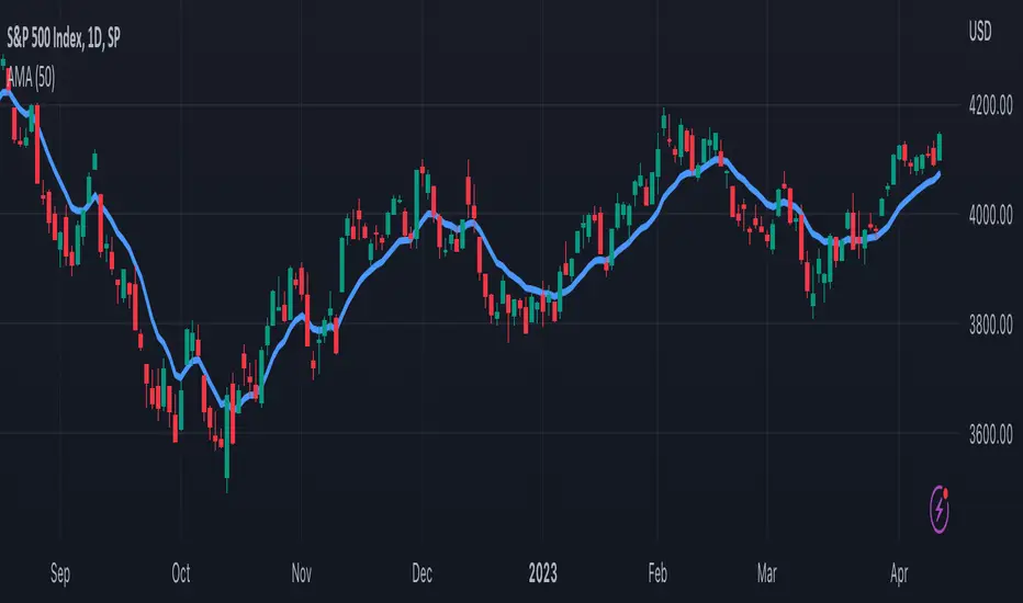
Aligned Moving Average IndexMoving averages are considered as aligned when either all faster moving averages are placed above their next slower moving averages or all faster moving averages are placed below their next slower moving averages. In this script, we are considering moving averages of 5, 10, 20, 30, 50, 100 and 200. User can select different moving average types from input : sma, ema, hma, rma, vwma, wma.
Moving average is considered as positively aligned when close > ma5 > ma10 > ma20 > ma30 > ma50 > ma100 > ma200
Moving average is considered as negatively aligned when close < ma5 < ma10 < ma20 < ma30 < ma50 < ma100 < ma200
Whenever there is positively aligned moving average, alignment value is considered as +1 and whenever there is negatively aligned moving average, alignment value is considered as -1. Aligned moving average index is sum of n periods of alignment value.
We can optionally apply another moving average on this index to see the overall direction.
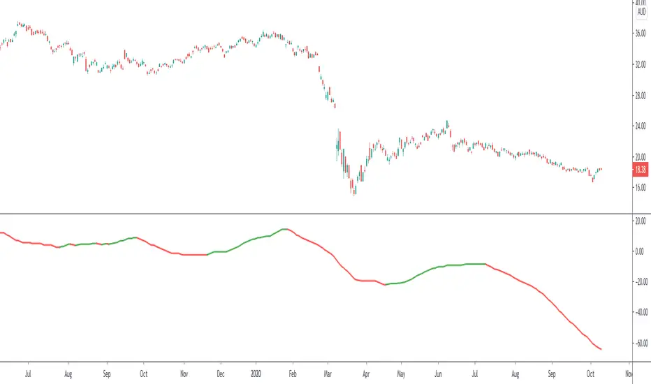
Savitzky-Golay Hampel Filter | AlphaNattSavitzky-Golay Hampel Filter | AlphaNatt
A revolutionary indicator combining NASA's satellite data processing algorithms with robust statistical outlier detection to create the most scientifically advanced trend filter available on TradingView.
"This is the same mathematics that processes signals from the Hubble Space Telescope and analyzes data from the Large Hadron Collider - now applied to financial markets."
━━━━━━━━━━━━━━━━━━━━━━━━━━━━━━━━━━━━━━━━
🚀 SCIENTIFIC PEDIGREE
Savitzky-Golay Filter Applications:
NASA: Satellite telemetry and space probe data processing
CERN: Particle physics data analysis at the LHC
Pharmaceutical: Chromatography and spectroscopy analysis
Astronomy: Processing signals from radio telescopes
Medical: ECG and EEG signal processing
Hampel Filter Usage:
Aerospace: Cleaning sensor data from aircraft and spacecraft
Manufacturing: Quality control in precision engineering
Seismology: Earthquake detection and analysis
Robotics: Sensor fusion and noise reduction
━━━━━━━━━━━━━━━━━━━━━━━━━━━━━━━━━━━━━━━━
🧬 THE MATHEMATICS
1. Savitzky-Golay Filter
The SG filter performs local polynomial regression on data points:
Fits a polynomial of degree n to a sliding window of data
Evaluates the polynomial at the center point
Preserves higher moments (peaks, valleys) unlike moving averages
Maintains derivative information for true momentum analysis
Originally published in Analytical Chemistry (1964)
Mathematical Properties:
Optimal smoothing in the least-squares sense
Preserves statistical moments up to polynomial order
Exact derivative calculation without additional lag
Superior frequency response vs traditional filters
2. Hampel Filter
A robust outlier detector based on Median Absolute Deviation (MAD):
Identifies outliers using robust statistics
Replaces spurious values with polynomial-fitted estimates
Resistant to up to 50% contaminated data
MAD is 1.4826 times more robust than standard deviation
Outlier Detection Formula:
|x - median| > k × 1.4826 × MAD
Where k is the threshold parameter (typically 3 for 99.7% confidence)
━━━━━━━━━━━━━━━━━━━━━━━━━━━━━━━━━━━━━━━━
💎 WHY THIS IS SUPERIOR
vs Moving Averages:
Preserves peaks and valleys (critical for catching tops/bottoms)
No lag penalty for smoothness
Maintains derivative information
Polynomial fitting > simple averaging
vs Other Filters:
Outlier immunity (Hampel component)
Scientifically optimal smoothing
Preserves higher-order features
Used in billion-dollar research projects
Unique Advantages:
Feature Preservation: Maintains market structure while smoothing
Spike Immunity: Ignores false breakouts and stop hunts
Derivative Accuracy: True momentum without additional indicators
Scientific Validation: 60+ years of academic research
━━━━━━━━━━━━━━━━━━━━━━━━━━━━━━━━━━━━━━━━
⚙️ PARAMETER OPTIMIZATION
1. Polynomial Order (2-5)
2 (Quadratic): Maximum smoothing, gentle curves
3 (Cubic): Balanced smoothing and responsiveness (recommended)
4-5 (Higher): More responsive, preserves more features
2. Window Size (7-51)
Must be odd number
Larger = smoother but more lag
Formula: 2×(desired smoothing period) + 1
Default 21 = analyzes 10 bars each side
3. Hampel Threshold (1.0-5.0)
1.0: Aggressive outlier removal (68% confidence)
2.0: Moderate outlier removal (95% confidence)
3.0: Conservative outlier removal (99.7% confidence) (default)
4.0+: Only extreme outliers removed
4. Final Smoothing (1-7)
Additional WMA smoothing after filtering
1 = No additional smoothing
3-5 = Recommended for most timeframes
7 = Ultra-smooth for position trading
━━━━━━━━━━━━━━━━━━━━━━━━━━━━━━━━━━━━━━━━
📊 TRADING STRATEGIES
Signal Recognition:
Cyan Line: Bullish trend with positive derivative
Pink Line: Bearish trend with negative derivative
Color Change: Trend reversal with polynomial confirmation
1. Trend Following Strategy
Enter when price crosses above cyan filter
Exit when filter turns pink
Use filter as dynamic stop loss
Best in trending markets
2. Mean Reversion Strategy
Enter long when price touches filter from below in uptrend
Enter short when price touches filter from above in downtrend
Exit at opposite band or filter color change
Excellent for range-bound markets
3. Derivative Strategy (Advanced)
The SG filter preserves derivative information
Acceleration = second derivative > 0
Enter on positive first derivative + positive acceleration
Exit on negative second derivative (momentum slowing)
━━━━━━━━━━━━━━━━━━━━━━━━━━━━━━━━━━━━━━━━
📈 PERFORMANCE CHARACTERISTICS
Strengths:
Outlier Immunity: Ignores stop hunts and flash crashes
Feature Preservation: Catches tops/bottoms better than MAs
Smooth Output: Reduces whipsaws significantly
Scientific Basis: Not curve-fitted or optimized to markets
Considerations:
Slight lag in extreme volatility (all filters have this)
Requires odd window sizes (mathematical requirement)
More complex than simple moving averages
Best with liquid instruments
━━━━━━━━━━━━━━━━━━━━━━━━━━━━━━━━━━━━━━━━
🔬 SCIENTIFIC BACKGROUND
Savitzky-Golay Publication:
"Smoothing and Differentiation of Data by Simplified Least Squares Procedures"
- Abraham Savitzky & Marcel Golay
- Analytical Chemistry, Vol. 36, No. 8, 1964
Hampel Filter Origin:
"Robust Statistics: The Approach Based on Influence Functions"
- Frank Hampel et al., 1986
- Princeton University Press
These techniques have been validated in thousands of scientific papers and are standard tools in:
NASA's Jet Propulsion Laboratory
European Space Agency
CERN (Large Hadron Collider)
MIT Lincoln Laboratory
Max Planck Institutes
━━━━━━━━━━━━━━━━━━━━━━━━━━━━━━━━━━━━━━━━
💡 ADVANCED TIPS
News Trading: Lower Hampel threshold before major events to catch spikes
Scalping: Use Order=2 for maximum smoothness, Window=11 for responsiveness
Position Trading: Increase Window to 31+ for long-term trends
Combine with Volume: Strong trends need volume confirmation
Multiple Timeframes: Use daily for trend, hourly for entry
Watch the Derivative: Filter color changes when first derivative changes sign
━━━━━━━━━━━━━━━━━━━━━━━━━━━━━━━━━━━━━━━━
⚠️ IMPORTANT NOTICES
Not financial advice - educational purposes only
Past performance does not guarantee future results
Always use proper risk management
Test settings on your specific instrument and timeframe
No indicator is perfect - part of complete trading system
━━━━━━━━━━━━━━━━━━━━━━━━━━━━━━━━━━━━━━━━
🏆 CONCLUSION
The Savitzky-Golay Hampel Filter represents the pinnacle of scientific signal processing applied to financial markets. By combining polynomial regression with robust outlier detection, traders gain access to the same mathematical tools that:
Guide spacecraft to other planets
Detect gravitational waves from black holes
Analyze particle collisions at near light-speed
Process signals from deep space
This isn't just another indicator - it's rocket science for trading .
"When NASA needs to separate signal from noise in billion-dollar missions, they use these exact algorithms. Now you can too."
━━━━━━━━━━━━━━━━━━━━━━━━━━━━━━━━━━━━━━━━
Developed by AlphaNatt
Version: 1.0
Release: 2025
Pine Script: v6
"Where Space Technology Meets Market Analysis"
Not financial advice. Always DYOR
Flexi MA Heat ZonesOverview
Flexi MA Heat Zones is a powerful multi-timeframe visualization tool that helps traders easily identify trend strength, direction, and potential zones of confluence using multiple moving averages and dynamic heatmaps. The indicator plots up to three pairs of customizable moving averages, with color-coded heat zones to highlight bullish and bearish conditions at a glance.
Whether you're a trend follower, mean-reversion trader, or looking for visual confirmation zones, this indicator is designed to offer deep insights with high customizability.
⚙️ Key Features
🔄 Supports multiple MA types: Choose from EMA, SMA, WMA, VWMA to suit your strategy.
🎯 Six moving averages: Three MA pairs (MA1-MA2, MA3-MA4, MA5-MA6), each with independent lengths and colors.
🌈 Heatmap Zones: Dynamic fills between MA pairs, changing color based on bullish or bearish alignment.
👁️🗨️ Full customization: Enable/disable any MA pair and its heatmap zone from the settings.
🪞 Transparency controls: Adjust the visibility of heat zones for clarity or stylistic preference.
🎨 Color-coded for clarity: Bullish and bearish colors for each heat zone pair, fully user-configurable.
🧩 Efficient layout: Smart use of grouped inputs for easier configuration and visibility management.
📈 How to Use
Use the MA1–MA2 and MA3–MA4 zones for longer-term trend tracking and confluence analysis.
Use the faster MA5–MA6 zone for short-term micro-trend identification or scalping.
When a faster MA is above the slower one within a pair, the fill turns bullish (user-defined color).
When the faster MA is below the slower one, the fill turns bearish.
Combine with price action or other indicators for entry/exit confirmation.
🧠 Pro Tips
For trend-following strategies, consider using EMA or WMA types.
For mean-reversion or support/resistance zones, SMA and VWMA may offer better zone clarity.
Overlay with RSI, MACD, or custom entry signals for higher confidence setups.
Use different heatmap transparencies to visually separate overlapping MA zones.

THF Crossover and Trend Signals Golden & Death Cross with VolumeScript Overview:
This Pine Script is designed to assist traders in identifying key buy/sell signals and major trend changes on the chart using Exponential Moving Averages (EMA) and Simple Moving Averages (SMA), as well as visualizing Golden Cross and Death Cross events. The script also includes a volume indicator to highlight the volume trading activity in relation to the price movements.
Key Features:
1. Moving Averages:
EMA 21: Exponential Moving Average over a 21-period, shown in green.
EMA 50: Exponential Moving Average over a 50-period, shown in yellow.
SMA 50: Simple Moving Average over a 50-period, shown in red.
SMA 200: Simple Moving Average over a 200-period, shown in blue.
2. Signals:
Buy Signal: Generated when EMA 21 crosses above SMA 50, indicating a potential upward trend. Displayed with a green label below the price bar.
Sell Signal: Generated when EMA 21 crosses below SMA 50, indicating a potential downward trend. Displayed with a red label above the price bar.
3. Golden Cross (Bullish Trend):
A Golden Cross occurs when EMA 50 crosses above SMA 200, which often signals the start of a long-term upward trend. The signal is displayed with a yellow label below the price bar.
4. Death Cross (Bearish Trend):
A Death Cross occurs when EMA 50 crosses below SMA 200, which often signals the start of a long-term downward trend. The signal is displayed with a blue label above the price bar.
5. Volume Indicator:
The volume is plotted as colored columns. Green indicates higher volume than the 20-period moving average, and red indicates lower volume.
A Volume Moving Average (SMA 20) is also plotted to compare volume changes over time.
How the Script Works:
1. The EMA and SMA lines are plotted on the chart, providing a visual representation of the short- and long-term trends.
2. Buy/Sell signals are triggered based on the crossover between EMA 21 and SMA 50, helping to identify potential entry and exit points.
3. The Golden Cross and Death Cross indicators highlight major trend reversals based on the crossover between EMA 50 and SMA 200, providing clear visual cues for long-term trend changes.
4. Volume is displayed alongside price movements, offering insight into the strength or weakness of a trend.
Key Customizations:
Moving Average Periods: Users can modify the lengths of the EMAs and SMAs for customized analysis.
Volume Moving Average Period: The script allows for adjustment of the volume moving average period to suit different market conditions.
Signal Visibility: The size and color of the buy, sell, Golden Cross, and Death Cross signals can be easily customized to make them more prominent on the chart.
Conclusion:
This script is ideal for traders looking to combine price action with volume analysis, using key technical indicators such as EMA, SMA, Golden Cross, and Death Cross to make informed decisions in trending markets.
---
This explanation covers all aspects of the script and provides a clear understanding of its functionality, which is helpful for sharing the script or using it as an educational resource.

Uptrick: Fusion Trend Reversion SystemOverview
The Uptrick: Fusion Trend Reversion System is a multi-layered indicator designed to identify potential price reversals during intraday movement while keeping traders informed of the dominant short-term trend. It blends a composite fair value model with deviation logic and a refined momentum filter using the Relative Strength Index (RSI). This tool was created with scalpers and short-term traders in mind and is especially effective on lower timeframes such as 1-minute, 5-minute, and 15-minute charts where price dislocations and quick momentum shifts are frequent.
Introduction
This indicator is built around the fusion of two classic concepts in technical trading: identifying trend direction and spotting potential reversion points. These are often handled separately, but this system merges them into one process. It starts by computing a fair value price using five moving averages, each with its own mathematical structure and strengths. These include the exponential moving average (EMA), which gives more weight to recent data; the simple moving average (SMA), which gives equal weight to all periods; the weighted moving average (WMA), which progressively increases weight with recency; the Arnaud Legoux moving average (ALMA), known for smoothing without lag; and the volume-weighted average price (VWAP), which factors in volume at each price level.
All five are averaged into a single value — the raw fusion line. This fusion acts as a dynamically balanced centerline that adapts to price conditions with both smoothing and responsiveness. Two additional exponential moving averages are applied to the raw fusion line. One is slower, giving a stable trend reference, and the other is faster, used to define momentum and cloud behavior. These two lines — the fusion slow and fusion fast — form the backbone of trend and signal logic.
Purpose
This system is meant for traders who want to trade reversals without losing sight of the underlying directional bias. Many reversal indicators fail because they act too early or signal too frequently in choppy markets. This script filters out noise through two conditions: price deviation and RSI confirmation. Reversion trades are considered only when the price moves a significant distance from fair value and RSI suggests a legitimate shift in momentum. That filtering process gives the trader a cleaner, higher-quality signal and reduces false entries.
The indicator also visually supports the trader through colored bars, up/down labels, and a filled cloud between the fast and slow fusion lines. These features make the market context immediately visible: whether the trend is up or down, whether a reversal just occurred, and whether price is currently in a high-risk reversion zone.
Originality and Uniqueness
What makes this script different from most reversal systems is the way it combines layers of logic — not just to detect signals, but to qualify and structure them. Rather than relying on a single MA or a raw RSI level, it uses a five-MA fusion to create a baseline fair value that incorporates speed, stability, and volume-awareness.
On top of that, the system introduces a dual-smoothing mechanism. It doesn’t just smooth price once — it creates two layers: one to follow the general trend and another to track faster deviations. This structure lets the script distinguish between continuation moves and possible turning points more effectively than a single-line or single-metric system.
It also uses RSI in a more refined way. Instead of just checking if RSI is overbought or oversold, the script smooths RSI and requires directional confirmation. Beyond that, it includes signal memory. Once a signal is generated, a new one will not appear unless the RSI becomes even more extreme and curls back again. This memory-based gating reduces signal clutter and prevents repetition, a rare feature in similar scripts.
Why these indicators were merged
Each moving average in the fusion serves a specific role. EMA reacts quickly to recent price changes and is often favored in fast-trading strategies. SMA acts as a long-term filter and smooths erratic behavior. WMA blends responsiveness with smoothing in a more balanced way. ALMA focuses on minimizing lag without losing detail, which is helpful in fast markets. VWAP anchors price to real trade volume, giving a sense of where actual positioning is happening.
By combining all five, the script creates a fair value model that doesn’t lean too heavily on one logic type. This fusion is then smoothed into two separate EMAs: one slower (trend layer), one faster (signal layer). The difference between these forms the basis of the trend cloud, which can be toggled on or off visually.
RSI is then used to confirm whether price is reversing with enough force to warrant a trade. The RSI is calculated over a 14-period window and smoothed with a 7-period EMA. The reason for smoothing RSI is to cut down on noise and avoid reacting to short, insignificant spikes. A signal is only considered if price is stretched away from the trend line and the smoothed RSI is in a reversal state — below 30 and rising for bullish setups, above 70 and falling for bearish ones.
Calculations
The script follows this structure:
Calculate EMA, SMA, WMA, ALMA, and VWAP using the same base length
Average the five values to form the raw fusion line
Smooth the raw fusion line with an EMA using sens1 to create the fusion slow line
Smooth the raw fusion line with another EMA using sens2 to create the fusion fast line
If fusion slow is rising and price is above it, trend is bullish
If fusion slow is falling and price is below it, trend is bearish
Calculate RSI over 14 periods
Smooth RSI using a 7-period EMA
Determine deviation as the absolute difference between current price and fusion slow
A raw signal is flagged if deviation exceeds the threshold
A raw signal is flagged if RSI EMA is under 30 and rising (bullish setup)
A raw signal is flagged if RSI EMA is over 70 and falling (bearish setup)
A final signal is confirmed for a bullish setup if RSI EMA is lower than the last bullish signal’s RSI
A final signal is confirmed for a bearish setup if RSI EMA is higher than the last bearish signal’s RSI
Reset the bullish RSI memory if RSI EMA rises above 30
Reset the bearish RSI memory if RSI EMA falls below 70
Store last signal direction and use it for optional bar coloring
Draw the trend cloud between fusion fast and fusion slow using fill()
Show signal labels only if showSignals is enabled
Bar and candle colors reflect either trend slope or last signal direction depending on mode selected
How it works
Once the script is loaded, it builds a fusion line by averaging five different types of moving averages. That line is smoothed twice into a fast and slow version. These two fusion lines form the structure for identifying trend direction and signal areas.
Trend bias is defined by the slope of the slow line. If the slow line is rising and price is above it, the market is considered bullish. If the slow line is falling and price is below it, it’s considered bearish.
Meanwhile, the script monitors how far price has moved from that slow line. If price is stretched beyond a certain distance (set by the threshold), and RSI confirms that momentum is reversing, a raw reversion signal is created. But the script only allows that signal to show if RSI has moved further into oversold or overbought territory than it did at the last signal. This blocks repetitive, weak entries. The memory is cleared only if RSI exits the zone — above 30 for bullish, below 70 for bearish.
Once a signal is accepted, a label is drawn. If the signal toggle is off, no label will be shown regardless of conditions. Bar colors are controlled separately — you can color them based on trend slope or last signal, depending on your selected mode.
Inputs
You can adjust the following settings:
MA Length: Sets the period for all moving averages used in the fusion.
Show Reversion Signals: Turns on the plotting of “Up” and “Down” labels when a reversal is confirmed.
Bar Coloring: Enables or disables colored bars based on trend or signal direction.
Show Trend Cloud: Fills the space between the fusion fast and slow lines to reflect trend bias.
Bar Color Mode: Lets you choose whether bars follow trend logic or last signal direction.
Sens 1: Smoothing speed for the slow fusion line — higher values = slower trend.
Sens 2: Smoothing speed for the fast line — lower values = faster signal response.
Deviation Threshold: Minimum distance price must move from fair value to trigger a signal check.
Features
This indicator offers:
A composite fair value model using five moving average types.
Dual smoothing system with user-defined sensitivity.
Slope-based trend definition tied to price position.
Deviation-triggered signal logic filtered by RSI reversal.
RSI memory system that blocks repetitive signals and resets only when RSI exits overbought or oversold zones.
Real-time tracking of the last signal’s direction for optional bar coloring.
Up/Down labels at signal points, visible only when enabled.
Optional trend cloud between fusion layers, visualizing current market bias.
Full user control over smoothing, threshold, color modes, and visibility.
Conclusion
The Fusion Trend-Reversion System is a tool for short-term traders looking to fade price extremes without ignoring trend bias. It calculates fair value using five diverse moving averages, smooths this into two dynamic layers, and applies strict reversal logic based on RSI deviation and momentum strength. Signals are triggered only when price is stretched and momentum confirms it with increasingly strong behavior. This combination makes the tool suitable for scalping, intraday entries, and fast market environments where precision matters.
Disclaimer
This indicator is for informational and educational purposes only. It does not constitute financial advice. All trading involves risk, and no tool can predict market behavior with certainty. Use proper risk management and do your own research before making trading decisions.

RSI-GringoRSI-Gringo — Stochastic RSI with Advanced Smoothing Averages
Overview:
RSI-Gringo is an advanced technical indicator that combines the concept of the Stochastic RSI with multiple smoothing options using various moving averages. It is designed for traders seeking greater precision in momentum analysis, while offering the flexibility to select the type of moving average that best suits their trading style.
Disclaimer: This script is not investment advice. Its use is entirely at your own risk. My responsibility is to provide a fully functional indicator, but it is not my role to guide how to trade, adjust, or use this tool in any specific strategy.
The JMA (Jurik Moving Average) version used in this script is a custom implementation based on publicly shared code by TradingView users, and it is not the original licensed version from Jurik Research.
What This Indicator Does
RSI-Gringo applies the Stochastic Oscillator logic to the RSI itself (rather than price), helping to identify overbought and oversold conditions within the RSI. This often leads to more responsive and accurate momentum signals.
This indicator displays:
%K: the main Stochastic RSI line
%D: smoothed signal line of %K
Upper/Lower horizontal reference lines at 80 and 20
Features and Settings
Available smoothing methods (selectable from dropdown):
SMA — Simple Moving Average
SMMA — Smoothed Moving Average (equivalent to RMA)
EMA — Exponential Moving Average
WMA — Weighted Moving Average
HMA — Hull Moving Average (manually implemented)
JMA — Jurik Moving Average (custom approximation)
KAMA — Kaufman Adaptive Moving Average
T3 — Triple Smoothed Moving Average with adjustable hot factor
How to Adjust Advanced Averages
T3 – Triple Smoothed MA
Parameter: T3 Hot Factor
Valid range: 0.1 to 2.0
Tuning:
Lower values (e.g., 0.1) make it faster but noisier
Higher values (e.g., 2.0) make it smoother but slower
Balanced range: 0.7 to 1.0 (recommended)
JMA – Jurik Moving Average (Custom)
Parameters:
Phase: adjusts responsiveness and smoothness (-100 to 100)
Power: controls smoothing intensity (default: 1)
Tuning:
Phase = 0: neutral behavior
Phase > 0: more reactive
Phase < 0: smoother, more delayed
Power = 1: recommended default for most uses
Note: The JMA used here is not the proprietary version by Jurik Research, but an educational approximation available in the public domain on TradingView.
How to Use
Crossover Signals
Buy signal: %K crosses above %D from below the 20 line
Sell signal: %K crosses below %D from above the 80 line
Momentum Strength
%K and %D above 80: strong bullish momentum
%K and %D below 20: strong bearish momentum
With Trend Filters
Combine this indicator with trend-following tools (like moving averages on price)
Fast smoothing types (like EMA or HMA) are better for scalping and day trading
Slower types (like T3 or KAMA) are better for swing and long-term trading
Final Tips
Tweak RSI and smoothing periods depending on the time frame you're trading.
Try different combinations of moving averages to find what works best for your strategy.
This indicator is intended as a supporting tool for technical analysis — not a standalone decision-making system.

Functionally Weighted Moving AverageOVERVIEW
An anchor-able moving average that weights historical prices with mathematical curves (shaping functions) such as Smoothstep , Ease In / Out , or even a Cubic Bézier . This level of configurability lends itself to more versatile price modeling, over conventional moving averages.
SESSION ANCHORS
Aside from VWAP, conventional moving averages do not allow you to use the first bar of each session as an anchor. This can make averages less useful near the open when price is sufficiently different from yesterdays close. For example, in this screenshot the EMA (blue) lags behind the sessionally anchored FWMA (yellow) at the open, making it slower to indicate a pivot higher.
An incrementing length is what makes a moving average anchor-able. VWAP is designed to do this, indefinitely growing until a new anchor resets the average (which is why it doesn't have a length parameter). But conventional MA's are designed to have a set length (they do not increment). Combining these features, the FWMA treats the length like a maximum rather than a set length, incrementing up to it from the anchor (when enabled).
Quick aside: If you code and want to anchor a conventional MA, the length() function in my UtilityLibrary will help you do this.
Incrementing an averages length introduces near-anchor volatility. For this reason, the FWMA also includes an option to saturate the anchor with the source , making values near the anchor more resistant to change. The following screenshot illustrates how saturation affects the average near the anchor when disabled (aqua) and enabled (fuchsia).
AVERAGING MATH
While there's nothing special about the math, it's worth documenting exactly how the average is affected by the anchor.
Average = Dot Product / Sum of Weights
Dot Product
This is the sum of element-wise multiplication between the Price and Weight arrays.
Dot Product = Price1 × Weight1 + Price2 × Weight2 + Price3 × Weight3 ...
When the Price and Weight arrays are equally sized (aka. the length is no longer incrementing from the anchor), there's a 1-1 mapping between Price and Weight indices. Anchoring, however, purges historical data from the Price array, making it temporarily smaller. When this happens, a dot product is synthesized by linearly interpolating for proportional indices (rather than a 1-1 mapping) to maintain the intended shape of weights.
Synthetic Dot Product = FirstPrice × FirstWeight + ... MidPrice × MidWeight ... + LastPrice × LastWeight
Sum of Weights
Exactly what it sounds like, the sum of weights used by the dot product operation. The sum of used weights may be less than the sum of all weights when the dot product is synthesized.
Sum of Weights = Weight1 + Weight2 + Weight3 ...
CALCULATING WEIGHTS
Shaping functions are mathematical curves used for interpolation. They are what give the Functionally Weighted Moving Average its name, and define how each historical price in the look back period is weighted.
The included shaping functions are:
Linear (conventional WMA)
Smoothstep (S curve)
Ease In Out (adjustable S curve)
Ease In (first half of Ease In Out)
Ease Out (second half of Ease In Out)
Ease Out In (eases out and then back in)
Cubic Bézier (aka. any curve you want)
In the following screenshot, the only difference between the three FWMA's is the shaping function (Ease In, Ease In Out, and Ease Out) illustrating how different curves can influence the responsiveness of an average.
And here is the same example, but with anchor saturation disabled .
ADJUSTING WEIGHTS
Each function outputs a range of values between 0 and 1. While you can't expand or shrink the range, you can nudge it higher or lower using the Scalar . For example, setting the scalar to -0.2 remaps to , and +0.2 remaps to . The following screenshot illustrates how -0.2 (lightest blue) and +0.2 (darkest blue) affect the average.
Easing functions can be further adjusted with the Degree (how much the shaping function curves). There's an interactive example of this here and the following illustrates how a degrees 0, 1, and 20 (dark orange, orange, and light orange) affect the average.
This level of configurability completely changes how a moving average models price for a given length, making the FWMA extremely versatile.
INPUTS
You can configure:
Length (how many historical bars to average)
Source (the bar value to average)
Offset (horizontal offset of the plot)
Weight (the shaping function)
Scalar (how much to adjust each weight)
Degree (how much to ease in / out)
Bézier Points (controls shape of Bézier)
Divisor & Anchor parameters
Style of the plot
BUT ... WHY?
We use moving averages to anticipate trend initialization, continuation, and termination. For a given look back period (length) we want the average to represent the data as accurately and smoothly as possible. The better it does this, the better it is at modeling price.
In this screenshot, both the FWMA (yellow) and EMA (blue) have a length of 9. They are both smooth, but one of them more accurately models price.
You wouldn't necessarily want to trade with these FWMA parameters, but knowing it does a better job of modeling price allows you to confidently expand the model to larger timeframes for bigger moves. Here, both the FWMA (yellow) and EMA (blue) have a length of 195 (aka. 50% of NYSE market hours).
INSPIRATION
I predominantly trade ETF derivatives and hold the position that markets are chaotic, not random . The salient difference being that randomness is entirely unpredictable, and chaotic systems can be modeled. The kind of analysis I value requires a very good pricing model.
The term "model" sounds more intimidating than it is. Math terms do that sometimes. It's just a mathematical estimation . That's it. For example, a regression is an "average regressing" model (aka. mean reversion ), and LOWESS (Locally Weighted Scatterplot Smoothing) is a statistically rigorous local regression .
LOWESS is excellent for modeling data. Also, it's not practical for trading. It's computationally expensive and uses data to the right of the point it's averaging, which is impossible in realtime (everything to the right is in the future). But many techniques used within LOWESS are still valuable.
My goal was to create an efficient real time emulation of LOWESS. Specifically I wanted something that was weighted non-linearly, was efficient, left-side only, and data faithful. Incorporate trading paradigms (like anchoring) and you get a Functionally Weighted Moving Average.
The formulas for determining the weights in LOWESS are typically chosen just because they seem to work well. Meaning ... they can be anything, and there's no justification other than "looks about right". So having a variety of functions (aka. kernels) for the FWMA, and being able to slide the weight range higher or lower, allows you to also make it "look about right".
William Cleveland, prominent figure in statistics known for his contributions to LOWESS, preferred using a tri-cube weighting function. Using Weight = Ease Out In with the Degrees = 3 is comparable to this. Enjoy!

EMA SuiteFor strategies with moving averages, of course. My preference is to use Fibonacci values, but it can be configured with any setup. When working on a single timeframe, it allows adding averages or groups of averages from other timeframes, I’ve used this for scalping. The indicator is designed to be dynamic and adaptable. By editing the script, it’s easy to add or remove averages.
Larger averages might slow down loading, and a color palette selector could be added since manually setting 11 values is tedious.
I’m open to any suggestions