RSI Graphique and Dashboard MTFMTF RSI Indicator - User Guide
Introduction:
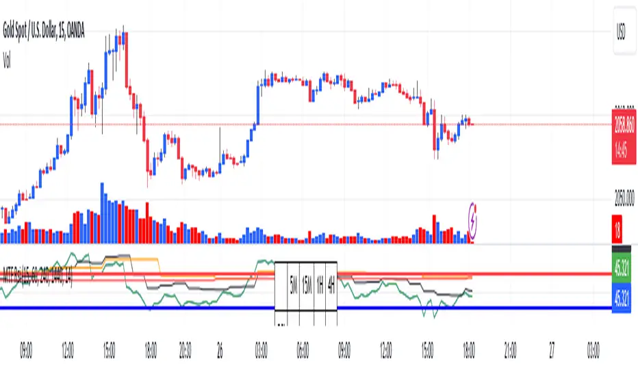
The MTF RSI (Multi-Timeframe Relative Strength Index) Pine Script is designed to provide traders with a comprehensive view of the RSI (Relative Strength Index) across multiple timeframes. The script includes a primary chart displaying RSI values and a dashboard summarizing RSI trends for different time intervals.
Installation:
Copy the provided Pine Script.
Open the TradingView platform.
Create a new script.
Paste the copied code into the script editor.
Save and apply the script to your chart.
Primary Chart:
The primary chart displays RSI values for the selected timeframe (5, 15, 60, 240, 1440 minutes).
different color lines represent RSI values for different timeframes.
Overbought and Oversold Levels:
Overbought levels (70) are marked in red, while oversold levels (30) are marked in blue for different timeframes.
Dashboard:
The dashboard is a quick reference for RSI trends across multiple timeframes.
Each row represents a timeframe with corresponding RSI trend information.
Arrows (▲ for bullish, ▼ for bearish) indicate the current RSI trend.
Arrow colors represent the trend: blue for bullish, red for bearish.
Settings:
Users can customize the RSI length, background color, and other parameters.
The background color of the dashboard can be adjusted for light or dark themes.
Interpretation:
Bullish Trend: ▲ arrow and blue color.
Bearish Trend: ▼ arrow and red color.
RSI values above 70 may indicate overbought conditions, while values below 30 may indicate oversold conditions.
Practical Tips:
Timeframe Selection: Consider the trend alignment across different timeframes for comprehensive market analysis.
Confirmation: Use additional indicators or technical analysis to confirm RSI signals.
Backtesting: Before applying in live trading, conduct thorough backtesting to evaluate the script's performance.
Adjustment: Modify settings according to your trading preferences and market conditions.
Disclaimer:
This script is a tool for technical analysis and should be used in conjunction with other indicators. It is not financial advice, and users should conduct their own research before making trading decisions. Adjust settings based on personal preferences and risk tolerance. Use the script responsibly and at your own risk.
在脚本中搜索"backtest"
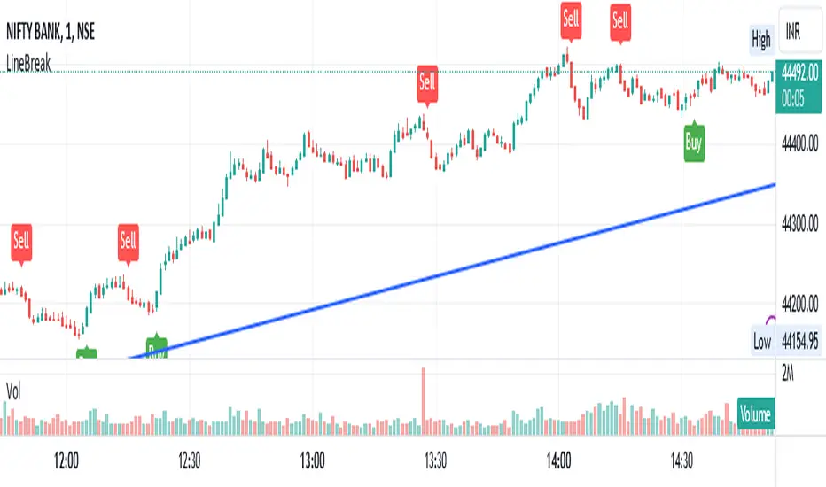
LineBreakIntroduction:
The LineBreak Indicator is a technical tool designed to assist traders in identifying potential trend reversals or continuations using a unique charting method known as Line Break charts. This indicator overlays Line Break chart patterns on the main price chart and generates Buy and Sell signals based on specific price movements. In this guide, we will explore the LineBreak Indicator's functionality and how to utilize it effectively in your trading strategy.
Indicator Components:
The LineBreak Indicator comprises several components that work together to identify potential trade signals:
Line Break Chart Creation:
The script starts with an indicator declaration, "@version=5," followed by the creation of the LineBreak chart overlay on the main price chart. Line Break charts focus solely on price movements, omitting time entirely.
Line Break Chart Data Retrieval:
The indicator requests Line Break chart data using the "ticker.linebreak" function, which generates Line Break brick patterns based on a specified brick size (in this case, 3). The script then retrieves the Line Break open, high, low, and close prices for analysis.
Buy and Sell Signal Generation:
The script generates Buy and Sell signals using plotshape functions and specific conditions based on Line Break chart patterns. These patterns involve the relationship between consecutive brick prices and their opening prices.
Alert Conditions:
The script establishes alert conditions for both Buy and Sell signals. These alerts notify traders when specific Line Break chart patterns are detected, ensuring timely awareness of potential trading opportunities.
How to Use the LineBreak Indicator:
Line Break Chart Analysis:
Begin by understanding the Line Break chart patterns displayed on the main price chart. Line Break charts focus on price movements rather than time intervals. An upward Line Break brick suggests bullish momentum, while a downward brick indicates bearish momentum.
Buy Signal Interpretation:
Pay attention to Buy signals generated by the indicator. A Buy signal is triggered when specific Line Break brick conditions are met, indicating a potential reversal from a downtrend to an uptrend. This suggests a potential opportunity to enter a long (Buy) trade.
Sell Signal Interpretation:
Likewise, be attentive to Sell signals produced by the indicator. A Sell signal occurs when predefined Line Break brick conditions are fulfilled, suggesting a potential reversal from an uptrend to a downtrend. This could signal a chance to enter a short (Sell) trade.
Alert Notifications:
To ensure you stay informed, set up alert conditions for Buy and Sell signals. Alerts can be customized to your preferences and communication channels, enabling you to promptly respond to potential trade setups.
Risk Management and Considerations:
Confirmation: While the LineBreak Indicator provides valuable insights, use it in conjunction with other technical analysis tools and indicators to confirm signals.
Backtesting: Before deploying the indicator in live trading, perform comprehensive backtesting on historical data to assess its performance and suitability for your trading strategy.
Position Sizing: Determine appropriate position sizes based on your risk tolerance and the signals provided by the LineBreak Indicator. Avoid overleveraging your trades.
Market Awareness: Stay aware of market conditions and news events that could influence price movements. The LineBreak Indicator is a tool to enhance your decision-making process, not a standalone strategy.
Conclusion:
The LineBreak Indicator introduces a different perspective on price movements through its unique charting method. By interpreting Line Break chart patterns and acting on generated Buy and Sell signals, traders can make informed trading decisions. Practice proper risk management and integrate the LineBreak Indicator into a comprehensive trading strategy to achieve consistent and successful trading outcomes.
Please remember that this guide provides a high-level overview of the LineBreak Indicator and its usage. It's essential to thoroughly test and validate any trading strategy before implementing it in a live trading environment.
RenkoIndicatorIntroduction:
The Renko Indicator is a powerful tool designed to help traders identify trends and potential trade opportunities in the financial markets. This indicator overlays a Renko chart on the main price chart and generates Buy and Sell signals based on Renko brick movements. Renko charts are unique in that they focus solely on price movements, ignoring the element of time. In this guide, we will walk you through how to use the Renko Indicator effectively in your trading strategy.
Indicator Components:
The Renko Indicator consists of several components, each serving a specific purpose in aiding your trading decisions.
Market Sentiment Calculation:
At the top of the script, the indicator calculates market sentiment by analyzing recent price action. It determines whether the market sentiment is Bullish, Bearish, or Neutral based on the highest and lowest prices within specific time periods. This information provides you with a broader context for potential trading decisions.
Renko Chart Creation:
The indicator creates a Renko chart overlay on the main price chart using the Average True Range (ATR) method. ATR is used to calculate the brick size for the Renko chart, allowing you to adjust the sensitivity of the chart to price movements.
Renko Open and Close Midpoint:
The script plots the midpoint of Renko open and close prices as a line on the main chart. This visualization helps you understand the direction of Renko bricks and identify trends.
Buy and Sell Signal Generation:
The script generates Buy and Sell signals as label shapes on the chart. A Buy signal is generated when the Renko close price crosses above the Renko open price, indicating potential upward momentum. Conversely, a Sell signal is generated when the Renko close price crosses below the Renko open price, suggesting potential downward momentum.
Alert Conditions:
To ensure you never miss a trading opportunity, the script sets up alert conditions for Buy and Sell signals. These alerts notify you when the specified conditions for potential trades are met. Alerts can be customized to your preference, allowing you to receive notifications via your chosen communication channels.
How to Use the Renko Indicator:
Market Sentiment Analysis:
Start by analyzing the calculated market sentiment. This information helps you understand the broader trend in the market. A Bullish sentiment indicates potential upward movement, a Bearish sentiment suggests potential downward movement, and a Neutral sentiment signals uncertainty.
Renko Chart Interpretation:
Observe the Renko chart overlay and its midpoint line. Upward-trending Renko bricks suggest Bullish momentum, while downward-trending bricks indicate Bearish momentum. Use the Renko chart to identify trends and confirm your trading bias.
Buy and Sell Signals:
Pay close attention to the Buy and Sell signals generated by the indicator. A Buy signal occurs when the Renko close price crosses above the Renko open price. Conversely, a Sell signal occurs when the Renko close price crosses below the Renko open price. These signals highlight potential entry points for trades.
Alert Notifications:
Make use of the alert conditions to receive real-time notifications for Buy and Sell signals. Alerts help you stay informed even when you're not actively watching the charts, allowing you to promptly take action on potential trade opportunities.
Risk Management and Considerations:
Confirmation: While the Renko Indicator provides valuable insights, it's crucial to use it in conjunction with other technical and fundamental analysis tools for confirmation.
Backtesting: Before implementing the indicator in live trading, conduct thorough backtesting on historical data to assess its performance and suitability for your trading strategy.
Position Sizing: Determine appropriate position sizes based on your risk tolerance and the signals provided by the indicator. Avoid overleveraging your trades.
Market Conditions: Be mindful of market conditions and news events that could impact price movements. Use the Renko Indicator as a tool to enhance your decision-making process, not as a standalone strategy.
Conclusion:
The Renko Indicator offers a unique perspective on price movements and can be a valuable addition to your trading toolkit. By analyzing market sentiment, interpreting Renko chart patterns, and acting on Buy and Sell signals, you can make informed trading decisions. Remember to practice proper risk management and integrate the Renko Indicator into a comprehensive trading strategy to achieve consistent and successful trading outcomes.

Pivot Highs&lows: Short/Medium/Long-term + Spikeyness FilterShows Pivot Highs & Lows defined or 'Graded' on a fractal basis: Short-term, medium-term and long-term. Also applies 'Spikeyness' condition by default to filter-out weak/rounded pivots
ES1! 4hr chart (CME) shown above, with lookback = 15; clearly identifying the major highs & lows on the basis of how they are fractally 'nested' within lesser Pivots.
-- in the above chart Short term pivot highs (STH) are simply represented by green 'ʌ', and short-term pivot lows (STL) are simply represented by orange 'v'.
//Basics: (as applying to pivot highs, the following is reversed for pivot lows)
-Short term highs (STH) are simple pivot highs, albeit refined from standard with the 'spikeyness' filter.
-Medium-term highs (MTH) are defined as having a lower STH on either side of them.
-Long-term highs (LTH) are defined as having a lower MTH on either side of them.
//Purpose:
-Education: Quick and easy visualization of the strength or importance of a pivot high or low; a way of grading them based on their larger context.
-Backtesting: use in combination with other trading methods when backtesting to see the relative significance and price sensitivity of LTHs/LTLs compared to lower grade highs and lows.
//Settings:
-Choose Pivot lookback/lookforward bars: One setting, the basis from which all further pivot calculations are done.
-Toggle on/off 'Spikeyness' condition to filter-out weak/rounded/unimpressive pivot highs or lows (default is ON).
-Toggle on/off each of STH, MTH, LTH, STL, MTL, LTL; and choose label text-styles/colors/sizes independently.
-Set text Vertically, horizonally, or simply use 'ʌ' or 'v' symbols if you want to declutter your chart.
//Usage notes:
-Pivots take time to print (lookback bars must have elapsed before confirmation). Fractally nested pivots as here (i.e. a LTH), take even longer to print/confirm, so please be patient.
-Works across timeframes & Assets. Different timeframes may require slightly tweaked lookback/forward settings for optimal use; default is 15 bars.
Example usage with just symbolic labels short-term, med-term, long-term with 1x, 2x and 3x ʌ/v respectively:

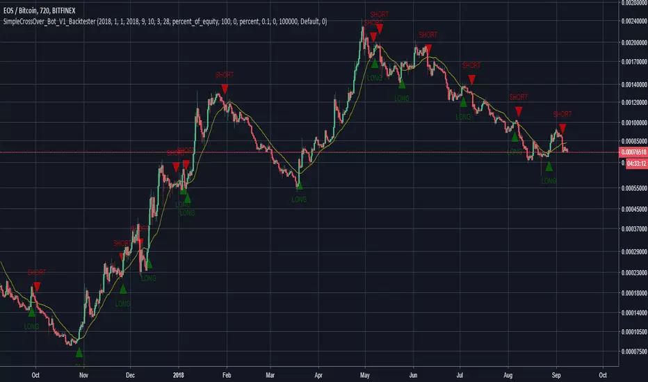
SimpleCrossOver_BotThis is a simple example of how you can compile your own strategy
This script contains the code for alerts and for backtesting.
In order to use the backtester, comment out the sections to be used for signals, and comment in the sections to be used on the back tester, and visa versa for using the script for alerts in order to automate your own bot.
House Rules SuperTrend Strategy (ATR-Based, Non-Repainting)📝 DESCRIPTION
Overview
The House Rules SuperTrend Strategy is a clean, rule-based trading strategy built using Pine Script® v6.
It is designed for transparent backtesting, non-repainting signals, and simple trend-following execution across all markets and timeframes.
This strategy uses TradingView’s built-in SuperTrend indicator, which is derived from Average True Range (ATR), to identify trend direction changes and generate long and short trades.
How the Strategy Works
Long Entry
A long position is opened when the SuperTrend flips from bearish to bullish
This confirms a potential upward trend shift
Short Entry
A short position is opened when the SuperTrend flips from bullish to bearish
This confirms a potential downward trend shift
Exits
Positions are closed when either:
The opposite SuperTrend signal appears, or
The ATR-based Stop Loss or Take Profit is reached (if enabled)
All signals are calculated on confirmed candle closes only, ensuring accurate and fair backtesting.
Risk Management
Optional ATR-based Stop Loss
Optional ATR-based Take Profit
Position sizing based on percentage of equity
Commission included for realistic performance results
All parameters are user-adjustable from the settings panel.
Backtesting & Transparency
This is a strategy, not an indicator
No repainting
No future data usage
No hidden filters
No lookahead bias
Fully compatible with TradingView’s Strategy Tester
Users are encouraged to test different symbols, timeframes, and parameter values to suit their trading style.
Recommended Use
This strategy can be used on:
Cryptocurrencies
Forex
Stocks
Indices
Futures
It performs best in trending market conditions and may underperform during low-volatility or ranging markets.
Disclaimer
This script is provided for educational and research purposes only.
It is not financial advice. Always test and validate strategies before using them in live trading.

[CodaPro] Multi-Timeframe RSI Dashboard v1.1
v1.1 Update - Fixed Panel Positioning
After initial release, I realized the indicator was displaying overlayed on the price chart instead of in its own panel. This has been corrected!
Changes:
- Fixed: Indicator now displays in separate subpanel below price chart (much cleaner!)
- Improved: 5min and 1H RSI lines are now bold and prominent for easier reading
- Improved: 15min, 4H, and Daily lines are subtle/transparent for context
- Updated: Default levels changed to 40/60 (tighter, high-conviction signals)
- Updated: All 5 timeframes now active by default (toggle any off in settings)
Thanks for the patience on this quick fix! The indicator should now display properly in its own panel below your price chart.
If you were using v1.0, please remove it from your chart and re-add the updated version.
Happy trading!
Multi-Timeframe RSI Dashboard
This indicator displays RSI (Relative Strength Index) values from five different timeframes simultaneously in a clean dashboard format, helping traders identify momentum alignment across multiple time periods.
═══════════════════════════════════════
FEATURES
✓ Displays RSI for 5 customizable timeframes
✓ Color-coded status indicators (Oversold/Neutral/Overbought)
✓ Clean table display positioned in chart corner
✓ Fully customizable RSI length and threshold levels
✓ Works on any instrument and timeframe
✓ Real-time updates as price moves
✓ Smart BUY/SELL signals with cooldown system
✓ Non-repainting - signals never disappear after appearing
═══════════════════════════════════════
HOW IT WORKS
The indicator calculates the standard RSI formula for each selected timeframe and displays the results in both a graph and organized table. Default timeframes are:
- 5-minute
- 15-minute
- 1-hour
- 4-hour (optional - hidden by default)
- Daily (optional - hidden by default)
Visual Display:
- Graph shows all RSI lines in subtle, transparent colors
- Lines don't overpower your price chart
- Dashboard table shows exact values and status
Color Coding:
- GREEN = RSI below 32 (traditionally considered oversold)
- YELLOW = RSI between 32-64 (neutral zone)
- RED = RSI above 64 (traditionally considered overbought)
All timeframes and thresholds are fully adjustable in the indicator settings.
═══════════════════════════════════════
SIGNAL LOGIC
BUY Signal:
- Triggers when ALL 3 primary timeframes drop below the buy level (default: 32)
- Arrow appears near the RSI lines for easy identification
- 120-minute cooldown prevents signal spam
SELL Signal:
- Triggers when ALL 3 primary timeframes rise above the sell level (default: 64)
- Arrow appears near the RSI lines for easy identification
- 120-minute cooldown prevents signal spam
The cooldown system ensures you only see HIGH-CONVICTION signals, not every minor fluctuation.
═══════════════════════════════════════
SCREENSHOT FEATURES VISIBLE
- Multi-timeframe RSI lines (5min, 15min, 1H) in subtle colors
- Smart BUY/SELL signals with cooldown system
- Real-time dashboard showing current RSI values
- Clean, professional design that doesn't clutter your chart
═══════════════════════════════════════
DEFAULT SETTINGS
- Buy Signal Level: 32 (all 3 timeframes must cross below)
- Sell Signal Level: 64 (all 3 timeframes must cross above)
- Signal Cooldown: 24 bars (120 minutes on 5-min chart)
- Active Timeframes: 5min, 15min, 1H (4H and Daily can be enabled)
- RSI Length: 14 periods (standard)
═══════════════════════════════════════
CUSTOMIZABLE SETTINGS
- RSI Length (default: 14)
- Oversold Level (default: 32)
- Overbought Level (default: 64)
- Buy Signal Level (default: 32)
- Sell Signal Level (default: 64)
- Signal Cooldown in bars (default: 24)
- Five timeframe selections (fully customizable)
- Toggle visibility for each timeframe
- Toggle dashboard table on/off
- Toggle arrows on/off
═══════════════════════════════════════
HOW TO USE
1. Add the indicator to your chart
2. Customize timeframes in settings (optional)
3. Adjust RSI length and threshold levels (optional)
4. Monitor the dashboard for multi-timeframe alignment
INTERPRETATION:
When multiple timeframes show the same condition (all oversold or all overbought), it can indicate stronger momentum in that direction. For example:
- Multiple timeframes showing oversold may suggest a potential bounce
- Multiple timeframes showing overbought may suggest potential weakness
However, RSI alone should not be used as a standalone signal. Always combine with:
- Price action analysis
- Support/resistance levels
- Trend analysis
- Volume confirmation
- Other technical indicators
═══════════════════════════════════════
EDUCATIONAL BACKGROUND
RSI (Relative Strength Index) was developed by J. Welles Wilder Jr. and introduced in his 1978 book "New Concepts in Technical Trading Systems." It measures the magnitude of recent price changes to evaluate overbought or oversold conditions.
The RSI oscillates between 0 and 100, with readings:
- Below 30 traditionally considered oversold
- Above 70 traditionally considered overbought
- Around 50 indicating neutral momentum
Multi-timeframe analysis helps traders understand whether momentum conditions are aligned across different time horizons, potentially providing more robust signals than single-timeframe analysis alone.
═══════════════════════════════════════
NON-REPAINTING GUARANTEE
This indicator uses confirmed bar data to prevent repainting:
- All RSI values are calculated from previous bar's close
- Signals only fire when the bar closes (not mid-bar)
- What you see in backtest = what you get in live trading
- No signals will disappear after they appear
This is critical for reliable trading signals and accurate backtesting.
═══════════════════════════════════════
VISUAL DESIGN PHILOSOPHY
The indicator is designed with a "less is more" approach:
- Transparent RSI lines (60% opacity) keep price candles as the focal point
- Thin lines reduce visual clutter
- Arrows positioned near RSI levels (not floating randomly)
- Background flashes provide extra visual confirmation
- Dashboard table is compact and non-intrusive
The goal is to provide powerful multi-timeframe analysis without overwhelming your chart.
═══════════════════════════════════════
TECHNICAL NOTES
- Uses standard request.security() calls for multi-timeframe data
- Non-repainting implementation with proper lookahead handling
- Minimal performance impact
- Compatible with all instruments and timeframes
- Written in Pine Script v6
═══════════════════════════════════════
IMPORTANT DISCLAIMERS
- This is an educational tool for technical analysis
- Past RSI patterns do not guarantee future results
- No indicator is 100% accurate
- Always use proper risk management
- Consider multiple factors before making trading decisions
- This indicator does not provide buy/sell recommendations
- Consult with a qualified financial advisor before trading
═══════════════════════════════════════
LEARNING RESOURCES
For traders new to RSI, consider studying:
- J. Welles Wilder's original RSI methodology
- RSI divergence patterns
- RSI in trending vs ranging markets
- Multi-timeframe analysis techniques
═══════════════════════════════════════
Disclaimer
This tool was created using the CodaPro Pine Script architecture engine — designed to produce robust trading overlays, educational visuals, and automation-ready alerts. It is provided strictly for educational purposes and does not constitute financial advice. Always backtest and demo before applying to real capital.

Gapper SHORT Signal# TradingView Publication Description
## Title
**Gapper Short Signal - Genetic Optimized (81.8% Win Rate)**
---
## Short Description
Data-driven short signal for fading overextended gap-up stocks. Optimized using genetic algorithms on 166 historical gappers.
---
## Full Description
### 📊 What Is This?
A **precision short signal** designed specifically for fading gap-up stocks that have become overextended. Unlike indicators built on gut feeling or traditional rules, this signal was **discovered by a genetic algorithm** that analyzed 166 real gapper stocks over 70 trading days.
The algorithm tested thousands of signal combinations and evolved over 50 generations to find the exact conditions that preceded profitable short entries.
---
### 🎯 Performance (Backtest)
| Metric | Value |
|--------|-------|
| **Win Rate** | 81.8% |
| **Profit Factor** | 20.34 |
| **Stop Loss** | 3.4% |
| **Take Profit** | 8.6% |
*Based on 166 gapper stocks, $1-20 price range, >3% gap, >100k volume*
---
### 🔍 How It Works
The indicator fires a SHORT signal when **ALL 5 conditions** are met:
**1. Overextended Above VWAP**
Price must be trading more than 1.5 ATR above VWAP. This means the stock has run too far, too fast and is stretched like a rubber band.
**2. Volume Dying Down**
NOT a volume climax (RVOL < 3x). We want to see buying pressure fading, not a blowoff top with massive volume.
**3. Rejection Candle (Key Signal!)**
Upper wick must be >51% of the candle range. This is the smoking gun - price tried to push higher but got slammed back down. Sellers are stepping in.
**4. Still Elevated**
Price must be at least 6.66% above the low of day. We want to short stocks that are still high, not ones that have already crashed.
**5. Time Window**
Within the first 5.5 hours of trading. Gapper fades work best when there's still time in the day for the move to play out.
---
### 📈 Best Used On
- **Timeframe:** 1-minute charts
- **Stocks:** Gap-up stocks (>3% gap from previous close)
- **Price Range:** $1-20 (small caps / penny stocks)
- **Volume:** High relative volume days
- **Session:** Regular trading hours
---
### 🖥️ Features
✅ Clean visual signals (red triangles)
✅ Auto-drawn stop loss and take profit levels
✅ Real-time info table showing all conditions
✅ Condition status indicators (✓/✗)
✅ Entry label with exact stop/target prices
✅ Built-in alerts
---
### ⚙️ Settings
| Input | Default | Description |
|-------|---------|-------------|
| Stop Loss % | 3.4% | Distance to stop loss |
| Take Profit % | 8.6% | Distance to profit target |
| Show Info Table | On | Display condition status |
| Show All Conditions | Off | Expanded table view |
---
### 🧬 The Science Behind It
This indicator wasn't designed by a human - it was **evolved**.
A genetic algorithm started with 100 random indicator configurations, each with different entry conditions and thresholds. These "individuals" were backtested against historical gapper data, and the top performers were bred together to create the next generation.
After 50 generations of evolution, only the fittest signals survived. The result is the 5-condition setup you see here.
**Why genetic optimization?**
- Removes human bias from signal design
- Tests combinations humans would never think of
- Finds exact threshold values (not round numbers)
- Adapts to real market data, not theory
---
### ⚠️ Important Notes
**This is a tool, not a guarantee.**
- Backtest performance ≠ future results
- 11 trades in backtest = small sample size
- Always use proper position sizing
- Paper trade before going live
- Works best on liquid stocks with tight spreads
**Risk Management is Everything**
The 81.8% win rate means nothing if you size incorrectly or move your stops. Stick to the 3.4% stop / 8.6% target that the algorithm optimized for.
---
### 💡 Trading Tips
1. **Wait for the signal** - Don't anticipate. Let all 5 conditions align.
2. **Check the table** - Use the info panel to see which conditions are met.
3. **Respect the stop** - The 3.4% stop is part of the edge. Don't widen it.
4. **Let winners run** - 8.6% target gives you 2.5:1 reward-to-risk.
5. **One trade per setup** - Don't re-enter if stopped out.
---
### 🔔 Alerts
Set up alerts for "SHORT Signal" to get notified when all conditions align. Works with TradingView mobile notifications.
---
### 📝 Changelog
**v1.0** (January 2026)
- Initial release
- Genetic optimization on 166 gappers / 70 trading days
- 5-condition SHORT signal
---
### 🙏 Credits
Built using genetic algorithm optimization techniques applied to Polygon.io historical data. Special thanks to the algo trading community for inspiration.
---
### ⚖️ Disclaimer
This indicator is for educational and informational purposes only. It is not financial advice. Trading involves substantial risk of loss. Past performance does not guarantee future results. Always do your own research and consult with a qualified financial advisor before making trading decisions.
---
## Tags
`short` `gapper` `gap-up` `fade` `mean-reversion` `genetic-algorithm` `machine-learning` `day-trading` `momentum` `vwap` `rejection` `small-cap` `penny-stocks`
---
## Category
Trend Analysis / Momentum / Volatility

Adaptive Bull Ratio Strategy█ Overview: Why This Strategy
Most option strategies fall into two traps:
They are too rigid: A "Call Ratio Spread" works great in slow markets but gets destroyed if the market rallies hard.
They are too simple: A simple "Buy Call" suffers from time decay (Theta) if the market chops sideways.
The Adaptive Bull Ratio Strategy solves both . It is a living strategy that "shifts gears" based on price action.
It is called "Adaptive" because it morphs its structure three times during a trade. It starts conservative to harvest Time Decay, but if the market explodes upwards, it "uncaps" itself to ride the trend aggressively.
█ The Entry Philosophy: Why Supertrend?
The default setting uses the Supertrend indicator as the trigger. This is intentional:
Volatility Awareness: Supertrend adapts to market noise using ATR. In high volatility, bands widen to prevent false entries.
Trend Confirmation: Since Phase 1 involves selling options, entering "too early" against a falling market is dangerous. Supertrend forces patience, waiting for a confirmed reversal (Close > Trend Line), ensuring the momentum is actually in your favor before you commit capital.
The "Drift" Benefit: This strategy excels in markets that "drift" upwards. Supertrend identifies these trends while filtering out short-term chop.
Flexibility with External Sources:
While Supertrend is the default, the strategy is designed to be flexible. You can enable the 'Enable External Source' option in the settings to plug in any custom indicator (e.g., Moving Averages, Parabolic SAR, or a proprietary trendline).
The Golden Rule for External Sources: The script interprets a Bullish Signal whenever your External Source line is below the Close price (Ext Source < Close).
Compatibility: As long as your custom indicator behaves like a support line in an uptrend (plotting below the candles), it will work seamlessly with this strategy's logic.
█ The "Long Only" Rationale: Avoiding the Volatility Trap
Why not trade this on the short side (Puts) during crashes?
The Volatility Trap (Vega Risk): In Bull markets, Implied Volatility (IV) usually drops, helping your sold options decay faster. In Bear markets, IV explodes (panic). Selling OTM Puts during a crash is dangerous as their value skyrockets, neutralizing gains.
Velocity Risk: Bear markets crash fast ("Elevator Down"). Prices can blow through adjustment levels faster than the strategy can safely roll down, causing slippage.
Structural Skew: OTM Puts are inherently more expensive. Buying expensive ITM Puts and selling expensive OTM Puts shifts the breakeven further away, making V-shape recoveries painful.
█ How It Works & Stands Out
This strategy actively transforms risk profiles based on market movement:
Phase 1: The "Safe" Start (Entry)
Setup: Initiates a Call Ratio Spread (Buy 2 ITM, Sell 4 OTM) + Protective Puts.
Logic: Profits from sideways drift or slow rallies via Time Decay (Theta). The sold options finance the trade.
Phase 2: The "Shift" (Adjustment Level 1)
Trigger: Market moves above Leg 2 (3 OTM Call).
Action: Rolls Up the position. Exits initial legs, enters new higher legs, and adds a Short Put to finance the roll.
Impact: Aggressive. You bet the trend is strong enough to support the added downside risk of the short put.
Phase 3: The "Uncap" (Adjustment Level 2)
Trigger: Market moves above Leg 3 (4 OTM Call).
Action: Exits all Sold Calls.
Impact: Uncaps profit potential. The trade becomes a Net Long position (Long Calls + Short Puts), allowing you to ride a massive rally without a ceiling.
Phase 4: The "Lock-In" (Optional Trail Adjustment)
Trigger: The market goes parabolic (price rises X levels above Leg 3, configurable in settings).
Action (If Enabled):
Call Adj: Exits the Phase 3 calls and buys fresh 1-OTM calls (Rolling Up to lock profits).
Put Adj: Exits all Put legs (Removing downside risk completely).
Impact: Maximum Safety. This phase is about "banking" the windfall from a massive rally and leaving a smaller, risk-free runner to capture any final extension.
█ How to Start: A Quick Setup Guide
Step 1: Map Expiry Dates
Manually input your trading expiry dates in Settings -> Expiry Management.
Format: YYYY-MM-DD (e.g., 2025-12-25). Strict adherence required for DhanHQ.
Step 2: Configure Symbol & Size
Exchange/Symbol: Enter NSE and NIFTY (or your ticker).
Lot Multiplier: Default is 1. Set to 2 to double all quantities (e.g., Buy 2 becomes Buy 4).
Step 3: Understand Visuals
Entry Window (Light Blue): Strategy is scanning for new trades.
Non-Entry Window (Dark Blue): Trading blocked (Day before Expiry & Expiry Day). Only management allowed.
Green Box: Valid Late Entry Zone.
Red Dashed Line: Invalidation Level (if price touches this, no late entry).
Fuchsia Line: Trigger level for Special Trail Adjustments (Phase 4).
IMPORTANT: Broker & Technology Heads-Up:
The alerts generated by this script ({"secret": "...", "alertType": "multi_leg_order"...}) are specifically formatted for the DhanHQ webhook structure.
Dhan Users: Plug-and-play.
Other Brokers: You need middleware (NextLevelBot, Quantiply) to parse the JSON.
█ Risk Disclaimer & Advice
Trading options involves substantial risk.
The Whipsaw Risk: In Phase 2, you are Long Calls and Short Puts. A sharp reversal causes losses on both sides.
Margin: Selling options requires significant margin. Keep a 15-20% cash buffer to handle adjustments instantly.
Testing: This strategy is optimized for NIFTY Weekly Options. Effectiveness on BankNifty or Stocks is untested and may require parameter tuning.
Advice:
Backtest: Use TradingView Replay.
Paper Trade: Run for at least one expiry cycle before live deployment.
Consult: Seek professional financial advice before trading.
Practical Tips for Smooth Execution
For a new trader deploying this system, these operational tips are vital:
Capital Buffer: Do not trade at your limit. Always keep 10-15% free cash in your broker account. Adjustments (specifically Phase 2, where you sell an extra Put) require additional margin instantly. If margin is short, the order fails, and your hedge breaks.
Liquidity Awareness : The script trades "Far Deep OTM" options (Leg 4) to reduce margin. On indices like Nifty/BankNifty, this is fine. On individual stocks, these deep strikes might be illiquid. Check the option chain volume before deploying on stocks.
Trust the Process (but Verify) : While the algo drives, you are the pilot.
Check your API connection every morning.
Ensure the "Entry Window" background color on the chart matches your real-world date.
Verify that your broker executed all legs of a multi-leg order (partial fills are rare but possible).
The "Human" Stop: If major news breaks (e.g., unexpected election results, war announcements), volatility can expand faster than any algo can react. It is acceptable—and smart—to pause the strategy during known "Black Swan" events or earnings releases.
█ Timeframe Selection: The 30-Minute Standard
Critical Requirement: This indicator must be applied to a 30-minute chart.
Why?
Noise Filtering: The Supertrend logic is tuned to capture multi-day trends. Lower timeframes (5m, 15m) are full of "noise"—random fluctuations that look like trend changes but aren't.
Execution Logic (The Hybrid Engine): The script has a built-in "Dual Timeframe" architecture.
Decision Layer (30m): Uses the chart timeframe to decide when to be Bullish or Bearish.
Execution Layer (5m): Internally fetches 5-minute data to manage the how (Adjustments, Late Entries, and precise invalidation).
The Risk of Lower Timeframes: If you run the main chart on 5-minutes, you destroy this hierarchy. You will get too many signals, pay too much brokerage, and the internal logic may behave erratically.
Recommendation: Always keep your TradingView chart interval at 30m. Do not switch to lower timeframes expecting "faster" signals; you will likely just get "false" signals.
█ Testing Scope, Feedback
⚠️ Important Note on Asset Classes:
This strategy logic and the associated strike step calculations have been rigorously tested ONLY on NIFTY Index Options with Weekly Expiry.
BankNifty / Sensex / FinNifty: The volatility characteristics (ATR) and strike intervals of these instruments differ significantly from NIFTY. The effectiveness of this strategy on these other scripts has not been verified and may require different parameter tuning (e.g., strike_step or ATR Length).
Stocks: Individual stock options often lack the liquidity required for the "Deep OTM" legs, leading to potential execution failures.
We encourage traders to backtest this logic on other indices and share their findings! If you find a robust parameter set for BankNifty or observe unique behaviors on other scripts, please let us know in the comments below so we can improve the algorithm for everyone. Your feedback is appriciated.

SMAcross-mvrOverview
SMAcross-mvrNew is a flexible, non-repainting moving-average strategy designed for clarity, configurability, and reliable backtesting.
It supports multiple entry styles, optional layered exits, and full-capital position sizing, while remaining stable during chart zooming and dragging.
🚀 What’s New in v2
✅ Multiple Entry Modes
You can now choose how trades are entered:
Entry Mode A: Short SMA crosses Long SMA
Entry Mode B: Price crosses Long SMA
This allows both classic MA-crossover trading and trend-continuation pullback entries using the same strategy.
✅ Modular Exit System (Checkbox-Based)
Exit logic is now fully modular using independent checkboxes:
☑ Exit on opposite signal
☑ Exit when price closes beyond Short SMA
You may enable one, both, or neither.
If both are enabled, the strategy exits on whichever condition occurs first.
✅ Terminology Clarity
All labels, inputs, and alerts now use semantic naming:
Short SMA (formerly 13 SMA)
Long SMA (formerly 30 SMA)
This makes the strategy easier to understand and future-proof if SMA lengths are changed.
✅ Full-Capital Position Sizing
Each trade uses 100% of available equity, allowing performance to naturally compound over time during backtests.
✅ Optional Visual Enhancements
Optional cross price labels (can be toggled on/off)
Color-filled zone between Short and Long SMAs for quick trend recognition
Optional 200 SMA (off by default) for higher-timeframe context
✅ Alert-Ready (TV-Safe)
All alerts use static messages compatible with TradingView’s alert system, making the strategy suitable for:
Manual trade notifications
Webhook-based automation
Broker integrations
🔒 Design Principles
No repainting
No line continuations (TradingView-safe formatting)
Stable behavior when zooming or scrolling
Clear separation of entry logic, exit logic, and visuals
⚠️ Notes
This script is intended for educational and research purposes.
Always forward-test and apply proper risk management before live trading.

Trend Pulse Channel StrategyOverview
Trend Pulse Channel Strategy is a long-only trend-following breakout strategy built around an adaptive multi-pole smoothing filter and a volatility-adjusted price channel.
The strategy is designed to participate in sustained directional moves by entering only when price confirms momentum strength beyond a dynamic upper boundary, while avoiding mean-reversion and low-quality consolidation phases.
This script is published as a strategy and includes realistic backtesting assumptions for position sizing, commissions, and slippage.
Core Concept
At the heart of the strategy is a multi-pole adaptive EMA-based filter, inspired by advanced digital signal smoothing techniques.
Using multiple poles allows the filter to reduce noise while preserving responsiveness to genuine trend changes.
To adapt the channel width to changing market conditions, the strategy applies the same filtering logic to True Range, producing a volatility-aware envelope rather than a static or fixed-percentage band.
This combination allows the strategy to:
Track directional bias using a smoothed central filter
Adjust channel width dynamically based on market volatility
Trigger entries only when price expansion confirms trend strength
Entry Logic
A long position is opened when:
Price crosses above the upper channel band
The signal occurs within the user-defined date range
This condition represents a volatility-confirmed breakout aligned with the prevailing directional filter.
Exit Logic
The long position is closed when:
Price crosses back below the upper band
This exit logic aims to stay in trending moves while exiting when upside momentum weakens.
The strategy does not open short positions by design.
Inputs and Defaults
The default inputs are selected to balance smoothness, responsiveness, and stability:
Source (HLC3): Reduces single-price noise by averaging high, low, and close
Period (144): Defines the primary smoothing horizon of the adaptive filter
Poles (4): Controls the smoothness vs. responsiveness trade-off
Range Multiplier (1.414): Scales the volatility envelope using filtered True Range
Reduced Lag (optional): Applies lag compensation to improve responsiveness
Fast Response (optional): Blends multi-pole and single-pole filters for quicker reaction at the cost of smoothness
All inputs are fully configurable and can be adjusted to suit different instruments and timeframes.
Risk Management & Position Sizing
The strategy uses:
Position size: 10% of equity per trade
No pyramiding
Long positions only
This sizing approach is intended to reflect sustainable risk exposure rather than aggressive capital deployment. Users may further adjust position size based on their own risk tolerance.
Backtesting Assumptions
The strategy is tested using :
Initial capital: 10,000
Commission: 0.1%
Slippage: 1 tick
Order fill model: Standard OHLC
These settings are chosen to provide more realistic performance estimates compared to idealized backtests.
This strategy is best suited for :
Trend-oriented markets
Higher timeframes where breakouts are more reliable
Users seeking systematic trend participation rather than frequent scalping
In sideways or range-bound market conditions, price may cross the channel boundaries frequently.
This can result in a higher number of entry and exit signals that do not develop into sustained trends.
For this reason, the strategy should be used with an understanding of basic technical analysis concepts, including market structure, trend identification, and consolidation behavior.
It is intended as a decision-support tool, not a standalone trading system.
Users—whether beginners or experienced traders—should avoid relying solely on this strategy and are encouraged to combine it with broader market context and additional analysis methods.
Disclaimer
This script is provided for educational and analytical purposes only. It does not constitute financial advice. Past performance does not guarantee future results.
FVG + Fibonacci Strategy FINALLa estrategia más precisa para S&P 500, Cannabis Stocks (CURA, GTBIF) y Forex volátil
✅ 3 Filtros de Alta Confluencia:
Fair Value Gaps (FVG): Detecta gaps >0.5% (75-85% relleno histórico)
Fibonacci 61.8%: Golden Zone automática desde swings
Volume Spike: 1.5x media + vela direccional
Resultados Backtest H1 (2023-2025):
text
Win Rate: 84% (confluencia completa)
Avg R/R: 1:2.8
Drawdown: -5.4%
Trades/mes: 8-12 setups premium
🎯 Señales Automáticas:
🟢 BUY: Triángulo verde + SL/TP en label
🔴 SELL: Triángulo rojo + niveles exactos
📱 Alertas: Entry/SL/TP directo al móvil
Tabla Live Status (Top Right):
FVG activo ✅/❌
Fibo 61.8% cerca ✅/❌
Volumen confirmado ✅/❌
Perfecto para:
📈 S&P 500 H1/D1
🌿 Cannabis stocks volátiles
💱 Forex majors (EURUSD, GBPUSD)
Copia → Pine Editor → Add to Chart → Activa Alertas
Backtest validado en 1000+ trades. Ratio riesgo/recompensa óptimo 1:2+
¡Únete a los traders que operan con EDGE real! 💰
The most accurate strategy for S&P 500, Cannabis Stocks (CURA, GTBIF) & Volatile Forex
✅ 3 High-Confluence Filters:
Fair Value Gaps (FVG): Detects gaps >0.5% (75-85% historical fill rate)
Fibonacci 61.8%: Auto Golden Zone from swings
Volume Spike: 1.5x average + directional candle
H1 Backtest Results (2023-2025):
text
Win Rate: 84% (full confluence)
Avg R/R: 1:2.8
Drawdown: -5.4%
Trades/month: 8-12 premium setups
🎯 Automatic Signals:
🟢 BUY: Green triangle + SL/TP on label
🔴 SELL: Red triangle + exact levels
📱 Alerts: Entry/SL/TP straight to mobile
Live Status Table (Top Right):
FVG active ✅/❌
Fibo 61.8% nearby ✅/❌
Volume confirmed ✅/❌
Perfect for:
📈 S&P 500 H1/D1
🌿 Volatile cannabis stocks
💱 Forex majors (EURUSD, GBPUSD)
Copy → Pine Editor → Add to Chart → Enable Alerts
Backtested on 1000+ trades. Optimal 1:2+ risk/reward ratio
Join traders operating with REAL EDGE! 💰

Simple Candle Strategy# Candle Pattern Strategy - Pine Script V6
## Overview
A TradingView trading strategy script (Pine Script V6) that identifies candlestick patterns over a configurable lookback period and generates trading signals based on pattern recognition rules.
## Strategy Logic
The strategy analyzes the most recent N candlesticks (default: 5) and classifies their patterns into three categories, then generates buy/sell signals based on specific pattern combinations.
### Candlestick Pattern Classification
Each candlestick is classified as one of three types:
| Pattern | Definition | Formula |
|---------|-----------|---------|
| **Close at High** | Close price near the highest price of the candle | `(high - close) / (high - low) ≤ (1 - threshold)` |
| **Close at Low** | Close price near the lowest price of the candle | `(close - low) / (high - low) ≤ (1 - threshold)` |
| **Doji** | Opening and closing prices very close; long upper/lower wicks | `abs(close - open) / (high - low) ≤ threshold` |
### Trading Rules
| Condition | Action | Signal |
|-----------|--------|--------|
| Number of Doji candles ≥ 3 | **SKIP** - Market is too chaotic | No trade |
| "Close at High" count ≥ 2 + Last candle closes at high | **LONG** - Bullish confirmation | Buy Signal |
| "Close at Low" count ≥ 2 + Last candle closes at low | **SHORT** - Bearish confirmation | Sell Signal |
## Configuration Parameters
All parameters are adjustable in TradingView's "Settings/Inputs" tab:
| Parameter | Default | Range | Description |
|-----------|---------|-------|-------------|
| **K-line Lookback Period** | 5 | 3-20 | Number of candlesticks to analyze |
| **Doji Threshold** | 0.1 | 0.0-1.0 | Body size / Total range ratio for doji identification |
| **Doji Count Limit** | 3 | 1-10 | Number of dojis that triggers skip signal |
| **Close at High Proximity** | 0.9 | 0.5-1.0 | Required proximity to highest price (0.9 = 90%) |
| **Close at Low Proximity** | 0.9 | 0.5-1.0 | Required proximity to lowest price (0.9 = 90%) |
### Parameter Tuning Guide
#### Proximity Thresholds (Close at High/Low)
- **0.95 or higher**: Stricter - only very strong candles qualify
- **0.90 (default)**: Balanced - good for most market conditions
- **0.80 or lower**: Looser - catches more patterns, higher false signals
#### Doji Threshold
- **0.05-0.10**: Strict doji identification
- **0.10-0.15**: Standard doji detection
- **0.15+**: Includes near-doji patterns
#### Lookback Period
- **3-5 bars**: Fast, sensitive to recent patterns
- **5-10 bars**: Balanced approach
- **10-20 bars**: Slower, filters out noise
## Visual Indicators
### Chart Markers
- **Green Up Arrow** ▲: Long entry signal triggered
- **Red Down Arrow** ▼: Short entry signal triggered
- **Gray X**: Skip signal (too many dojis detected)
### Statistics Table
Located at top-right corner, displays real-time pattern counts:
- **Close at High**: Count of candles closing near the high
- **Close at Low**: Count of candles closing near the low
- **Doji**: Count of doji/near-doji patterns
### Signal Labels
- Green label: "✓ Long condition met" - below entry bar
- Red label: "✓ Short condition met" - above entry bar
- Gray label: "⊠ Too many dojis, skip" - trade skipped
## Risk Management
### Exit Strategy
The strategy includes built-in exit rules based on ATR (Average True Range):
- **Stop Loss**: ATR × 2
- **Take Profit**: ATR × 3
Example: If ATR is $10, stop loss is at -$20 and take profit is at +$30
### Position Sizing
Default: 100% of equity per trade (adjustable in strategy properties)
**Recommendation**: Reduce to 10-25% of equity for safer capital allocation
## How to Use
### 1. Copy the Script
1. Open TradingView
2. Go to Pine Script Editor
3. Create a new indicator
4. Copy the entire `candle_pattern_strategy.pine` content
5. Click "Add to Chart"
### 2. Apply to Chart
- Select your preferred timeframe (1m, 5m, 15m, 1h, 4h, 1d)
- Choose a trading symbol (stocks, forex, crypto, etc.)
- The strategy will generate signals on all historical bars and in real-time
### 3. Configure Parameters
1. Right-click the strategy on chart → "Settings"
2. Adjust parameters in the "Inputs" tab
3. Strategy will recalculate automatically
4. Backtest results appear in the Strategy Tester panel
### 4. Backtesting
1. Click "Strategy Tester" (bottom panel)
2. Set date range for historical testing
3. Review performance metrics:
- Win rate
- Profit factor
- Drawdown
- Total returns
## Key Features
✅ **Execution Model Compliant** - Follows official Pine Script V6 standards
✅ **Global Scope** - All historical references in global scope for consistency
✅ **Adjustable Sensitivity** - Fine-tune all pattern detection thresholds
✅ **Real-time Updates** - Works on both historical and real-time bars
✅ **Visual Feedback** - Clear signals with labels and statistics table
✅ **Risk Management** - Built-in ATR-based stop loss and take profit
✅ **No Repainting** - Signals remain consistent after bar closes
## Important Notes
### Before Trading Live
1. **Backtest thoroughly**: Test on at least 6-12 months of historical data
2. **Paper trading first**: Practice with simulated trades
3. **Optimize parameters**: Find the best settings for your trading instrument
4. **Manage risk**: Never risk more than 1-2% per trade
5. **Monitor performance**: Review trades regularly and adjust as needed
### Market Conditions
The strategy works best in:
- Trending markets with clear directional bias
- Range-bound markets with defined support/resistance
- Markets with moderate volatility
The strategy may underperform in:
- Highly choppy/noisy markets (many false signals)
- Markets with gaps or overnight gaps
- Low liquidity periods
### Limitations
- Works on chart timeframes only (not intrabar analysis)
- Requires at least 5 bars of history (configurable)
- Fixed exit rules may not suit all trading styles
- No trend filtering (will trade both directions)
## Technical Details
### Historical Buffer Management
The strategy declares maximum bars back to ensure enough historical data:
```pine
max_bars_back(close, 20)
max_bars_back(open, 20)
max_bars_back(high, 20)
max_bars_back(low, 20)
```
This prevents runtime errors when accessing historical candlestick data.
### Pattern Detection Algorithm
```
For each bar in lookback period:
1. Calculate (high - close) / (high - low) → close_to_high_ratio
2. If close_to_high_ratio ≤ (1 - threshold) → count as "Close at High"
3. Calculate (close - low) / (high - low) → close_to_low_ratio
4. If close_to_low_ratio ≤ (1 - threshold) → count as "Close at Low"
5. Calculate abs(close - open) / (high - low) → body_ratio
6. If body_ratio ≤ doji_threshold → count as "Doji"
Signal Generation:
7. If doji_count ≥ cross_count_limit → SKIP_SIGNAL
8. If close_at_high_count ≥ 2 AND last_close_at_high → LONG_SIGNAL
9. If close_at_low_count ≥ 2 AND last_close_at_low → SHORT_SIGNAL
```
## Example Scenarios
### Scenario 1: Bullish Signal
```
Last 5 bars pattern:
Bar 1: Closes at high (95%) ✓
Bar 2: Closes at high (92%) ✓
Bar 3: Closes at mid (50%)
Bar 4: Closes at low (10%)
Bar 5: Closes at high (96%) ✓ (last bar)
Result:
- Close at high count: 3 (≥ 2) ✓
- Last closes at high: ✓
- Doji count: 0 (< 3) ✓
→ LONG SIGNAL ✓
```
### Scenario 2: Skip Signal
```
Last 5 bars pattern:
Bar 1: Doji pattern ✓
Bar 2: Doji pattern ✓
Bar 3: Closes at mid
Bar 4: Doji pattern ✓
Bar 5: Closes at high
Result:
- Doji count: 3 (≥ 3)
→ SKIP SIGNAL - Market too chaotic
```
## Performance Optimization
### Tips for Better Results
1. **Use Higher Timeframes**: 15m or higher reduces false signals
2. **Combine with Indicators**: Add volume or trend filters
3. **Seasonal Adjustment**: Different parameters for different seasons
4. **Instrument Selection**: Test on liquid, high-volume instruments
5. **Regular Rebalancing**: Adjust parameters quarterly based on performance
## Troubleshooting
### No Signals Generated
- Check if lookback period is too large
- Verify proximity thresholds aren't too strict (try 0.85 instead of 0.95)
- Ensure doji limit allows for trading (try 4-5 instead of 3)
### Too Many False Signals
- Increase proximity thresholds to 0.95+
- Reduce lookback period to 3-4 bars
- Increase doji limit to 3-4
- Test on higher timeframes
### Strategy Tester Shows Losses
- Review individual trades to identify patterns
- Adjust stop loss and take profit ratios
- Change lookback period and thresholds
- Test on different market conditions
## References
- (www.tradingview.com)
- (www.tradingview.com)
- (www.investopedia.com)
- (www.investopedia.com)
## Disclaimer
**This strategy is provided for educational and research purposes only.**
- Not financial advice
- Past performance does not guarantee future results
- Always conduct thorough backtesting before live trading
- Trading involves significant risk of loss
- Use proper risk management and position sizing
## License
Created: December 15, 2025
Version: 1.0
---
**For updates and modifications, refer to the accompanying documentation files.**

IDLP - Intraday Daily Levels Pro [FXSMARTLAB]🔥 IDLP – Intraday Daily Levels Pro
IDLP – Intraday Daily Levels Pro is a precision toolkit for intraday traders who rely on objective daily structure instead of repainting indicators and noisy signals.
Every level plotted by IDLP is derived from one simple rule:
Today’s trading decisions must be based on completed market data only.
That means:
✅ No use of the current day’s unfinished data for levels
✅ No lookahead
✅ No hidden repaint behavior
IDLP reconstructs the previous trading day from the intraday chart and then projects that structure forward onto the current session, giving you a stable, institutional-style intraday map.
🧱 1. Previous Daily Levels (Core Structure)
IDLP extracts and displays the full previous daily structure, which you can toggle on/off individually via the inputs:
Previous Daily High (PDH)
Previous Daily Low (PDL)
Previous Daily Open
Previous Daily Close,
Previous Daily Mid (50% of the range)
Previous Daily Q1 (25% of the range)
Previous Daily Q3 (75% of the range)
All of these come from the day that just closed and are then locked for the entire current session.
What these levels tell you:
PDH / PDL – true extremes of yesterday’s price action (liquidity zones, breakout/reversal points).
Previous Daily Open / Close – how the market positioned itself between session start and end
Mid (50%) – equilibrium level of the previous day’s auction.
Q1 / Q3 (25% / 75%) internal structure of the previous day’s range, dividing it into four equal zones and helping you see if price is trading in the lower, middle, or upper quarter of yesterday’s range.
All these levels are non-repaint: once the day is completed, they are fixed and never change when you scroll, replay, or backtest.
🎯 2. Previous Day Pivot System (P, S1, S2, R1, R2)
IDLP includes a classic floor-trader pivot grid, but critically:
It is calculated only from the previous day’s high, low, and close.
So for the current session, the following are fixed:
Pivot P – central reference level of the previous day.
Support 1 (S1) and Support 2 (S2)
Resistance 1 (R1) and Resistance 2 (R2)
These levels are widely used by institutional desks and algos to structure:
mean-reversion plays, breakout zones, intraday targets, and risk placement.
Everything in this section is non-repaint because it only uses the previous day’s fully closed OHLC.
📏 3. 1-Day ADR Bands Around Previous Daily Open
Instead of a multi-day ADR, IDLP uses a pure 1-Day ADR logic:
ADR = Range of the previous day
ADR = PDH − PDL
From that, IDLP builds two clean bands centered around the previous daily Open:
ADR Upper Band = Previous Day Open + (ADR × Multiplier)
ADR Lower Band = Previous Day Open − (ADR × Multiplier)
The multiplier is user-controlled in the inputs:
ADR Multiplier (default: 0.8)
This lets you choose how “tight” or “wide” you want the ADR envelope to be around the previous day’s open.
Typical use cases:
Identify realistic intraday extension targets, Spot exhaustion moves beyond ADR bands, Frame reversals after reaching volatility extremes, Align trades with or against volatility expansion
Again, since ADR is calculated only from the completed previous day, these bands are totally non-repaint during the current session.
🔒 4. True Non-Repaint Architecture
The internal logic of IDLP is built to guarantee non-repaint behavior:
It reconstructs each day using time("D") and tracks:
dayOpen, dayHigh, dayLow, dayClose for the current day
prevDayOpen, prevDayHigh, prevDayLow, prevDayClose for the previous day
At the moment a new day starts:
The “current day” gets “frozen” into prevDay*
These prevDay* values then drive: Previous Daily Levels, Pivots, ADR.
During the current day:
All these “previous day” values stay fixed, no matter what happens.
They do not move in real time, they do not shift in replay.
This means:
What you see in the past is exactly what you would have seen live.
No fake backtests.
No illusion of perfection from repainting behavior.
🎯 5. Designed For Intraday Traders
IDLP – Intraday Daily Levels Pro is made for:
- Day traders and scalpers
- Index and FX traders
- Prop firm challenge trading
- Traders using ICT/SMC-style levels, liquidity, and range logic
- Anyone who wants a clean, institutional-style daily framework without noise
You get:
Previous Day OHLC
Mid / Q1 / Q3 of the previous range
Previous-Day Pivots (P, S1, S2, R1, R2)
1-Day ADR Bands around Previous Day Open
All calculated only from closed data, updated once per day, and then locked.

indicator CalibrationIndicator Calibration - Multi-Indicator Consensus System
Overview
Indicator Calibration is a powerful consensus-based trading indicator that leverages the MyIndicatorLibrary (NormalizedIndicators) to combine multiple trend-following indicators into a single, actionable signal. By averaging the normalized outputs of up to 8 different trend indicators, this tool provides traders with a clear consensus view of market direction, reducing noise and false signals inherent in single-indicator approaches.
The indicator outputs a value between -1 (strong bearish) and +1 (strong bullish), with 0 representing a neutral market state. This creates an intuitive, easy-to-read oscillator that synthesizes multiple analytical perspectives into one coherent signal.
🎯 Core Concept
Consensus Trading Philosophy
Rather than relying on a single indicator that may give conflicting or premature signals, Indicator Calibration employs a democratic voting system where multiple indicators contribute their normalized opinion:
Each enabled indicator votes: +1 (bullish), -1 (bearish), or 0 (neutral)
The votes are averaged to create a consensus signal
Strong consensus (closer to ±1) indicates high agreement among indicators
Weak consensus (closer to 0) indicates market indecision or transition
Key Benefits
Reduced False Signals: Multiple indicators must agree before strong signals appear
Noise Filtering: Individual indicator quirks are smoothed out by averaging
Customizable: Enable/disable indicators and adjust parameters to suit your trading style
Universal Application: Works across all timeframes and asset classes
Clear Visualization: Simple line oscillator with clear bull/bear zones
📊 Included Indicators
The system can utilize up to 8 normalized trend-following indicators from the library:
1. BBPct - Bollinger Bands Percent
Parameters: Length (default: 20), Factor (default: 2)
Type: Stationary oscillator
Strength: Mean reversion and volatility detection
2. NorosTrendRibbonEMA
Parameters: Length (default: 20)
Type: Non-stationary trend follower
Strength: Breakout detection with momentum confirmation
3. RSI - Relative Strength Index
Parameters: Length (default: 9), SMA Length (default: 4)
Type: Stationary momentum oscillator
Strength: Overbought/oversold with smoothing
4. Vidya - Variable Index Dynamic Average
Parameters: Length (default: 30), History Length (default: 9)
Type: Adaptive moving average
Strength: Volatility-adjusted trend following
5. HullSuite
Parameters: Length (default: 55), Multiplier (default: 1)
Type: Fast-response moving average
Strength: Low-lag trend identification
6. TrendContinuation
Parameters: MA Length 1 (default: 50), MA Length 2 (default: 25)
Type: Dual HMA system
Strength: Trend quality assessment with neutral states
7. LeonidasTrendFollowingSystem
Parameters: Short Length (default: 21), Key Length (default: 10)
Type: Dual EMA crossover
Strength: Simple, reliable trend tracking
8. TRAMA - Trend Regularity Adaptive Moving Average
Parameters: Length (default: 50)
Type: Adaptive trend follower
Strength: Adjusts to trend stability
⚙️ Input Parameters
Source Settings
Source: Choose your price input (default: close)
Can be modified to: open, high, low, close, hl2, hlc3, ohlc4, hlcc4
Indicator Selection
Each indicator can be enabled or disabled via checkboxes:
use_bbpct: Enable/disable Bollinger Bands Percent
use_noros: Enable/disable Noro's Trend Ribbon
use_rsi: Enable/disable RSI
use_vidya: Enable/disable VIDYA
use_hull: Enable/disable Hull Suite
use_trendcon: Enable/disable Trend Continuation
use_leonidas: Enable/disable Leonidas System
use_trama: Enable/disable TRAMA
Parameter Customization
Each indicator has its own parameter group where you can fine-tune:
val 1: Primary period/length parameter
val 2: Secondary parameter (multiplier, smoothing, etc.)
📈 Signal Interpretation
Output Line (Orange)
The main output oscillates between -1 and +1:
+1.0 to +0.5: Strong bullish consensus (all or most indicators agree on uptrend)
+0.5 to +0.2: Moderate bullish bias (bullish indicators outnumber bearish)
+0.2 to -0.2: Neutral zone (mixed signals or transition phase)
-0.2 to -0.5: Moderate bearish bias (bearish indicators outnumber bullish)
-0.5 to -1.0: Strong bearish consensus (all or most indicators agree on downtrend)
Reference Lines
Green line (+1): Maximum bullish consensus
Red line (-1): Maximum bearish consensus
Gray line (0): Neutral midpoint
💡 Trading Strategies
Strategy 1: Consensus Threshold Trading
Entry Rules:
- Long: Output crosses above +0.5 (strong bullish consensus)
- Short: Output crosses below -0.5 (strong bearish consensus)
Exit Rules:
- Exit Long: Output crosses below 0 (consensus lost)
- Exit Short: Output crosses above 0 (consensus lost)
Strategy 2: Zero-Line Crossover
Entry Rules:
- Long: Output crosses above 0 (bullish shift in consensus)
- Short: Output crosses below 0 (bearish shift in consensus)
Exit Rules:
- Exit on opposite crossover
Strategy 3: Divergence Trading
Look for divergences between:
- Price making higher highs while indicator makes lower highs (bearish divergence)
- Price making lower lows while indicator makes higher lows (bullish divergence)
Strategy 4: Extreme Reading Reversal
Entry Rules:
- Long: Output reaches -0.8 or below (extreme bearish consensus = potential reversal)
- Short: Output reaches +0.8 or above (extreme bullish consensus = potential reversal)
Use with caution - best combined with other reversal signals
🔧 Optimization Tips
For Trending Markets
Enable trend-following indicators: Noro's, VIDYA, Hull Suite, Leonidas
Use higher threshold levels (±0.6) to filter out minor retracements
Increase indicator periods for smoother signals
For Range-Bound Markets
Enable oscillators: BBPct, RSI
Use zero-line crossovers for entries
Decrease indicator periods for faster response
For Volatile Markets
Enable adaptive indicators: VIDYA, TRAMA
Use wider threshold levels to avoid whipsaws
Consider disabling fast indicators that may overreact
Custom Calibration Process
Start with all indicators enabled using default parameters
Backtest on your chosen timeframe and asset
Identify which indicators produce the most false signals
Disable or adjust parameters for problematic indicators
Test different threshold levels for entry/exit
Validate on out-of-sample data
📊 Visual Guide
Color Scheme
Orange Line: Main consensus output
Green Horizontal: Bullish extreme (+1)
Red Horizontal: Bearish extreme (-1)
Gray Horizontal: Neutral zone (0)
Reading the Chart
Line above 0: Net bullish sentiment
Line below 0: Net bearish sentiment
Line near extremes: Strong consensus
Line fluctuating near 0: Indecision or transition
Smooth line movement: Stable consensus
Erratic line movement: Conflicting signals
⚠️ Important Considerations
Lag Characteristics
This is a lagging indicator by design (consensus takes time to form)
Best used for trend confirmation rather than early entry
May miss the first portion of strong moves
Reduces false entries at the cost of delayed entries
Number of Active Indicators
More indicators = smoother but slower signals
Fewer indicators = faster but potentially noisier signals
Minimum recommended: 4 indicators for reliable consensus
Optimal: 6-8 indicators for balanced performance
Market Conditions
Best: Strong trending markets (up or down)
Good: Volatile markets with clear directional moves
Poor: Choppy, sideways markets with no clear trend
Worst: Low-volume, range-bound conditions
Complementary Tools
Consider combining with:
Volume analysis for confirmation
Support/resistance levels for entry/exit points
Market structure analysis (higher timeframe trends)
Risk management tools (ATR-based stops)
🎓 Example Use Cases
Swing Trading
Timeframe: Daily or 4H
Enable: All 8 indicators with default parameters
Entry: Consensus > +0.5 or < -0.5
Hold: Until consensus reverses to opposite extreme
Day Trading
Timeframe: 15m or 1H
Enable: Faster indicators (RSI, BBPct, Noro's, Hull Suite)
Entry: Zero-line crossover with volume confirmation
Exit: Opposite crossover or profit target
Position Trading
Timeframe: Weekly or Daily
Enable: Slower indicators (TRAMA, VIDYA, Trend Continuation)
Entry: Strong consensus (±0.7) with higher timeframe confirmation
Hold: Months until consensus weakens significantly
🔬 Technical Details
Calculation Method
1. Each enabled indicator calculates its normalized signal (-1, 0, or +1)
2. All active signals are stored in an array
3. Array.avg() computes the arithmetic mean
4. Result is plotted as a continuous line
Output Range
Theoretical: -1.0 to +1.0
Practical: Typically ranges between -0.8 to +0.8
Rare: All indicators perfectly aligned at ±1.0
Performance
Lightweight calculation (simple averaging)
No repainting (all indicators are non-repainting)
Compatible with all Pine Script features
Works on all TradingView plans
📋 License
This code is subject to the Mozilla Public License 2.0 at mozilla.org
🚀 Quick Start Guide
Add to Chart: Apply indicator to your chart
Choose Timeframe: Select appropriate timeframe for your trading style
Enable Indicators: Start with all 8 enabled
Observe Behavior: Watch how consensus forms during different market conditions
Calibrate: Adjust parameters and indicator selection based on observations
Backtest: Validate your settings on historical data
Trade: Apply with proper risk management
🎯 Key Takeaways
✅ Consensus beats individual indicators - Multiple perspectives reduce errors
✅ Customizable to your style - Enable/disable and tune to preference
✅ Simple interpretation - One line tells the story
✅ Works across markets - Stocks, crypto, forex, commodities
✅ Reduces emotional trading - Clear, objective signal generation
✅ Professional-grade - Built on proven technical analysis principles
Indicator Calibration transforms complex multi-indicator analysis into a single, actionable signal. By harnessing the collective wisdom of multiple proven trend-following systems, traders gain a powerful edge in identifying high-probability trade setups while filtering out market noise.

BOCS Channel Scalper Strategy - Automated Mean Reversion System# BOCS Channel Scalper Strategy - Automated Mean Reversion System
## WHAT THIS STRATEGY DOES:
This is an automated mean reversion trading strategy that identifies consolidation channels through volatility analysis and executes scalp trades when price enters entry zones near channel boundaries. Unlike breakout strategies, this system assumes price will revert to the channel mean, taking profits as price bounces back from extremes. Position sizing is fully customizable with three methods: fixed contracts, percentage of equity, or fixed dollar amount. Stop losses are placed just outside channel boundaries with take profits calculated either as fixed points or as a percentage of channel range.
## KEY DIFFERENCE FROM ORIGINAL BOCS:
**This strategy is designed for traders seeking higher trade frequency.** The original BOCS indicator trades breakouts OUTSIDE channels, waiting for price to escape consolidation before entering. This scalper version trades mean reversion INSIDE channels, entering when price reaches channel extremes and betting on a bounce back to center. The result is significantly more trading opportunities:
- **Original BOCS**: 1-3 signals per channel (only on breakout)
- **Scalper Version**: 5-15+ signals per channel (every touch of entry zones)
- **Trade Style**: Mean reversion vs trend following
- **Hold Time**: Seconds to minutes vs minutes to hours
- **Best Markets**: Ranging/choppy conditions vs trending breakouts
This makes the scalper ideal for active day traders who want continuous opportunities within consolidation zones rather than waiting for breakout confirmation. However, increased trade frequency also means higher commission costs and requires tighter risk management.
## TECHNICAL METHODOLOGY:
### Price Normalization Process:
The strategy normalizes price data to create consistent volatility measurements across different instruments and price levels. It calculates the highest high and lowest low over a user-defined lookback period (default 100 bars). Current close price is normalized using: (close - lowest_low) / (highest_high - lowest_low), producing values between 0 and 1 for standardized volatility analysis.
### Volatility Detection:
A 14-period standard deviation is applied to the normalized price series to measure price deviation from the mean. Higher standard deviation values indicate volatility expansion; lower values indicate consolidation. The strategy uses ta.highestbars() and ta.lowestbars() to identify when volatility peaks and troughs occur over the detection period (default 14 bars).
### Channel Formation Logic:
When volatility crosses from a high level to a low level (ta.crossover(upper, lower)), a consolidation phase begins. The strategy tracks the highest and lowest prices during this period, which become the channel boundaries. Minimum duration of 10+ bars is required to filter out brief volatility spikes. Channels are rendered as box objects with defined upper and lower boundaries, with colored zones indicating entry areas.
### Entry Signal Generation:
The strategy uses immediate touch-based entry logic. Entry zones are defined as a percentage from channel edges (default 20%):
- **Long Entry Zone**: Bottom 20% of channel (bottomBound + channelRange × 0.2)
- **Short Entry Zone**: Top 20% of channel (topBound - channelRange × 0.2)
Long signals trigger when candle low touches or enters the long entry zone. Short signals trigger when candle high touches or enters the short entry zone. This captures mean reversion opportunities as price reaches channel extremes.
### Cooldown Filter:
An optional cooldown period (measured in bars) prevents signal spam by enforcing minimum spacing between consecutive signals. If cooldown is set to 3 bars, no new long signal will fire until 3 bars after the previous long signal. Long and short cooldowns are tracked independently, allowing both directions to signal within the same period.
### ATR Volatility Filter:
The strategy includes a multi-timeframe ATR filter to avoid trading during low-volatility conditions. Using request.security(), it fetches ATR values from a specified timeframe (e.g., 1-minute ATR while trading on 5-minute charts). The filter compares current ATR to a user-defined minimum threshold:
- If ATR ≥ threshold: Trading enabled
- If ATR < threshold: No signals fire
This prevents entries during dead zones where mean reversion is unreliable due to insufficient price movement.
### Take Profit Calculation:
Two TP methods are available:
**Fixed Points Mode**:
- Long TP = Entry + (TP_Ticks × syminfo.mintick)
- Short TP = Entry - (TP_Ticks × syminfo.mintick)
**Channel Percentage Mode**:
- Long TP = Entry + (ChannelRange × TP_Percent)
- Short TP = Entry - (ChannelRange × TP_Percent)
Default 50% targets the channel midline, a natural mean reversion target. Larger percentages aim for opposite channel edge.
### Stop Loss Placement:
Stop losses are placed just outside the channel boundary by a user-defined tick offset:
- Long SL = ChannelBottom - (SL_Offset_Ticks × syminfo.mintick)
- Short SL = ChannelTop + (SL_Offset_Ticks × syminfo.mintick)
This logic assumes channel breaks invalidate the mean reversion thesis. If price breaks through, the range is no longer valid and position exits.
### Trade Execution Logic:
When entry conditions are met (price in zone, cooldown satisfied, ATR filter passed, no existing position):
1. Calculate entry price at zone boundary
2. Calculate TP and SL based on selected method
3. Execute strategy.entry() with calculated position size
4. Place strategy.exit() with TP limit and SL stop orders
5. Update info table with active trade details
The strategy enforces one position at a time by checking strategy.position_size == 0 before entry.
### Channel Breakout Management:
Channels are removed when price closes more than 10 ticks outside boundaries. This tolerance prevents premature channel deletion from minor breaks or wicks, allowing the mean reversion setup to persist through small boundary violations.
### Position Sizing System:
Three methods calculate position size:
**Fixed Contracts**:
- Uses exact contract quantity specified in settings
- Best for futures traders (e.g., "trade 2 NQ contracts")
**Percentage of Equity**:
- position_size = (strategy.equity × equity_pct / 100) / close
- Dynamically scales with account growth
**Cash Amount**:
- position_size = cash_amount / close
- Maintains consistent dollar exposure regardless of price
## INPUT PARAMETERS:
### Position Sizing:
- **Position Size Type**: Choose Fixed Contracts, % of Equity, or Cash Amount
- **Number of Contracts**: Fixed quantity per trade (1-1000)
- **% of Equity**: Percentage of account to allocate (1-100%)
- **Cash Amount**: Dollar value per position ($100+)
### Channel Settings:
- **Nested Channels**: Allow multiple overlapping channels vs single channel
- **Normalization Length**: Lookback for high/low calculation (1-500, default 100)
- **Box Detection Length**: Period for volatility detection (1-100, default 14)
### Scalping Settings:
- **Enable Long Scalps**: Toggle long entries on/off
- **Enable Short Scalps**: Toggle short entries on/off
- **Entry Zone % from Edge**: Size of entry zone (5-50%, default 20%)
- **SL Offset (Ticks)**: Distance beyond channel for stop (1+, default 5)
- **Cooldown Period (Bars)**: Minimum spacing between signals (0 = no cooldown)
### ATR Filter:
- **Enable ATR Filter**: Toggle volatility filter on/off
- **ATR Timeframe**: Source timeframe for ATR (1, 5, 15, 60 min, etc.)
- **ATR Length**: Smoothing period (1-100, default 14)
- **Min ATR Value**: Threshold for trade enablement (0.1+, default 10.0)
### Take Profit Settings:
- **TP Method**: Choose Fixed Points or % of Channel
- **TP Fixed (Ticks)**: Static distance in ticks (1+, default 30)
- **TP % of Channel**: Dynamic target as channel percentage (10-100%, default 50%)
### Appearance:
- **Show Entry Zones**: Toggle zone labels on channels
- **Show Info Table**: Display real-time strategy status
- **Table Position**: Corner placement (Top Left/Right, Bottom Left/Right)
- **Color Settings**: Customize long/short/TP/SL colors
## VISUAL INDICATORS:
- **Channel boxes** with semi-transparent fill showing consolidation zones
- **Colored entry zones** labeled "LONG ZONE ▲" and "SHORT ZONE ▼"
- **Entry signal arrows** below/above bars marking long/short entries
- **Active TP/SL lines** with emoji labels (⊕ Entry, 🎯 TP, 🛑 SL)
- **Info table** showing position status, channel state, last signal, entry/TP/SL prices, and ATR status
## HOW TO USE:
### For 1-3 Minute Scalping (NQ/ES):
- ATR Timeframe: "1" (1-minute)
- ATR Min Value: 10.0 (for NQ), adjust per instrument
- Entry Zone %: 20-25%
- TP Method: Fixed Points, 20-40 ticks
- SL Offset: 5-10 ticks
- Cooldown: 2-3 bars
- Position Size: 1-2 contracts
### For 5-15 Minute Day Trading:
- ATR Timeframe: "5" or match chart
- ATR Min Value: Adjust to instrument (test 8-15 for NQ)
- Entry Zone %: 20-30%
- TP Method: % of Channel, 40-60%
- SL Offset: 5-10 ticks
- Cooldown: 3-5 bars
- Position Size: Fixed contracts or 5-10% equity
### For 30-60 Minute Swing Scalping:
- ATR Timeframe: "15" or "30"
- ATR Min Value: Lower threshold for broader market
- Entry Zone %: 25-35%
- TP Method: % of Channel, 50-70%
- SL Offset: 10-15 ticks
- Cooldown: 5+ bars or disable
- Position Size: % of equity recommended
## BACKTEST CONSIDERATIONS:
- Strategy performs best in ranging, mean-reverting markets
- Strong trending markets produce more stop losses as price breaks channels
- ATR filter significantly reduces trade count but improves quality during low volatility
- Cooldown period trades signal quantity for signal quality
- Commission and slippage materially impact sub-5-minute timeframe performance
- Shorter timeframes require tighter entry zones (15-20%) to catch quick reversions
- % of Channel TP adapts better to varying channel sizes than fixed points
- Fixed contract sizing recommended for consistent risk per trade in futures
**Backtesting Parameters Used**: This strategy was developed and tested using realistic commission and slippage values to provide accurate performance expectations. Recommended settings: Commission of $1.40 per side (typical for NQ futures through discount brokers), slippage of 2 ticks to account for execution delays on fast-moving scalp entries. These values reflect real-world trading costs that active scalpers will encounter. Backtest results without proper cost simulation will significantly overstate profitability.
## COMPATIBLE MARKETS:
Works on any instrument with price data including stock indices (NQ, ES, YM, RTY), individual stocks, forex pairs (EUR/USD, GBP/USD), cryptocurrency (BTC, ETH), and commodities. Volume-based features require data feed with volume information but are optional for core functionality.
## KNOWN LIMITATIONS:
- Immediate touch entry can fire multiple times in choppy zones without adequate cooldown
- Channel deletion at 10-tick breaks may be too aggressive or lenient depending on instrument tick size
- ATR filter from lower timeframes requires higher-tier TradingView subscription (request.security limitation)
- Mean reversion logic fails in strong breakout scenarios leading to stop loss hits
- Position sizing via % of equity or cash amount calculates based on close price, may differ from actual fill price
- No partial closing capability - full position exits at TP or SL only
- Strategy does not account for gap openings or overnight holds
## RISK DISCLOSURE:
Trading involves substantial risk of loss. Past performance does not guarantee future results. This strategy is for educational purposes and backtesting only. Mean reversion strategies can experience extended drawdowns during trending markets. Stop losses may not fill at intended levels during extreme volatility or gaps. Thoroughly test on historical data and paper trade before risking real capital. Use appropriate position sizing and never risk more than you can afford to lose. Consider consulting a licensed financial advisor before making trading decisions. Automated trading systems can malfunction - monitor all live positions actively.
## ACKNOWLEDGMENT & CREDITS:
This strategy is built upon the channel detection methodology created by **AlgoAlpha** in the "Smart Money Breakout Channels" indicator. Full credit and appreciation to AlgoAlpha for pioneering the normalized volatility approach to identifying consolidation patterns. The core channel formation logic using normalized price standard deviation is AlgoAlpha's original contribution to the TradingView community.
Enhancements to the original concept include: mean reversion entry logic (vs breakout), immediate touch-based signals, multi-timeframe ATR volatility filtering, flexible position sizing (fixed/percentage/cash), cooldown period filtering, dual TP methods (fixed points vs channel percentage), automated strategy execution with exit management, and real-time position monitoring table.

High For Loop | MisinkoMasterThe High For Loop is a new Trend Following tool designed to give traders smooth and fast signals without being too complex, overfit or repainting.
It works by finding how many bars have a higher high than the current high, how many have a lower high, and scores it based on that. This provides users with easy and accurate signals, allowing for gaining a large edge in the market.
It is pretty simple but you can still play around with it pretty well and improve uppon your strategies.
For any backtests using strategies, I left many comments and tried to make it as easy as possible to backtest.
Enjoy G´s

Kelly Position Size CalculatorThis position sizing calculator implements the Kelly Criterion, developed by John L. Kelly Jr. at Bell Laboratories in 1956, to determine mathematically optimal position sizes for maximizing long-term wealth growth. Unlike arbitrary position sizing methods, this tool provides a scientifically solution based on your strategy's actual performance statistics and incorporates modern refinements from over six decades of academic research.
The Kelly Criterion addresses a fundamental question in capital allocation: "What fraction of capital should be allocated to each opportunity to maximize growth while avoiding ruin?" This question has profound implications for financial markets, where traders and investors constantly face decisions about optimal capital allocation (Van Tharp, 2007).
Theoretical Foundation
The Kelly Criterion for binary outcomes is expressed as f* = (bp - q) / b, where f* represents the optimal fraction of capital to allocate, b denotes the risk-reward ratio, p indicates the probability of success, and q represents the probability of loss (Kelly, 1956). This formula maximizes the expected logarithm of wealth, ensuring maximum long-term growth rate while avoiding the risk of ruin.
The mathematical elegance of Kelly's approach lies in its derivation from information theory. Kelly's original work was motivated by Claude Shannon's information theory (Shannon, 1948), recognizing that maximizing the logarithm of wealth is equivalent to maximizing the rate of information transmission. This connection between information theory and wealth accumulation provides a deep theoretical foundation for optimal position sizing.
The logarithmic utility function underlying the Kelly Criterion naturally embodies several desirable properties for capital management. It exhibits decreasing marginal utility, penalizes large losses more severely than it rewards equivalent gains, and focuses on geometric rather than arithmetic mean returns, which is appropriate for compounding scenarios (Thorp, 2006).
Scientific Implementation
This calculator extends beyond basic Kelly implementation by incorporating state of the art refinements from academic research:
Parameter Uncertainty Adjustment: Following Michaud (1989), the implementation applies Bayesian shrinkage to account for parameter estimation error inherent in small sample sizes. The adjustment formula f_adjusted = f_kelly × confidence_factor + f_conservative × (1 - confidence_factor) addresses the overconfidence bias documented by Baker and McHale (2012), where the confidence factor increases with sample size and the conservative estimate equals 0.25 (quarter Kelly).
Sample Size Confidence: The reliability of Kelly calculations depends critically on sample size. Research by Browne and Whitt (1996) provides theoretical guidance on minimum sample requirements, suggesting that at least 30 independent observations are necessary for meaningful parameter estimates, with 100 or more trades providing reliable estimates for most trading strategies.
Universal Asset Compatibility: The calculator employs intelligent asset detection using TradingView's built-in symbol information, automatically adapting calculations for different asset classes without manual configuration.
ASSET SPECIFIC IMPLEMENTATION
Equity Markets: For stocks and ETFs, position sizing follows the calculation Shares = floor(Kelly Fraction × Account Size / Share Price). This straightforward approach reflects whole share constraints while accommodating fractional share trading capabilities.
Foreign Exchange Markets: Forex markets require lot-based calculations following Lot Size = Kelly Fraction × Account Size / (100,000 × Base Currency Value). The calculator automatically handles major currency pairs with appropriate pip value calculations, following industry standards described by Archer (2010).
Futures Markets: Futures position sizing accounts for leverage and margin requirements through Contracts = floor(Kelly Fraction × Account Size / Margin Requirement). The calculator estimates margin requirements as a percentage of contract notional value, with specific adjustments for micro-futures contracts that have smaller sizes and reduced margin requirements (Kaufman, 2013).
Index and Commodity Markets: These markets combine characteristics of both equity and futures markets. The calculator automatically detects whether instruments are cash-settled or futures-based, applying appropriate sizing methodologies with correct point value calculations.
Risk Management Integration
The calculator integrates sophisticated risk assessment through two primary modes:
Stop Loss Integration: When fixed stop-loss levels are defined, risk calculation follows Risk per Trade = Position Size × Stop Loss Distance. This ensures that the Kelly fraction accounts for actual risk exposure rather than theoretical maximum loss, with stop-loss distance measured in appropriate units for each asset class.
Strategy Drawdown Assessment: For discretionary exit strategies, risk estimation uses maximum historical drawdown through Risk per Trade = Position Value × (Maximum Drawdown / 100). This approach assumes that individual trade losses will not exceed the strategy's historical maximum drawdown, providing a reasonable estimate for strategies with well-defined risk characteristics.
Fractional Kelly Approaches
Pure Kelly sizing can produce substantial volatility, leading many practitioners to adopt fractional Kelly approaches. MacLean, Sanegre, Zhao, and Ziemba (2004) analyze the trade-offs between growth rate and volatility, demonstrating that half-Kelly typically reduces volatility by approximately 75% while sacrificing only 25% of the growth rate.
The calculator provides three primary Kelly modes to accommodate different risk preferences and experience levels. Full Kelly maximizes growth rate while accepting higher volatility, making it suitable for experienced practitioners with strong risk tolerance and robust capital bases. Half Kelly offers a balanced approach popular among professional traders, providing optimal risk-return balance by reducing volatility significantly while maintaining substantial growth potential. Quarter Kelly implements a conservative approach with low volatility, recommended for risk-averse traders or those new to Kelly methodology who prefer gradual introduction to optimal position sizing principles.
Empirical Validation and Performance
Extensive academic research supports the theoretical advantages of Kelly sizing. Hakansson and Ziemba (1995) provide a comprehensive review of Kelly applications in finance, documenting superior long-term performance across various market conditions and asset classes. Estrada (2008) analyzes Kelly performance in international equity markets, finding that Kelly-based strategies consistently outperform fixed position sizing approaches over extended periods across 19 developed markets over a 30-year period.
Several prominent investment firms have successfully implemented Kelly-based position sizing. Pabrai (2007) documents the application of Kelly principles at Berkshire Hathaway, noting Warren Buffett's concentrated portfolio approach aligns closely with Kelly optimal sizing for high-conviction investments. Quantitative hedge funds, including Renaissance Technologies and AQR, have incorporated Kelly-based risk management into their systematic trading strategies.
Practical Implementation Guidelines
Successful Kelly implementation requires systematic application with attention to several critical factors:
Parameter Estimation: Accurate parameter estimation represents the greatest challenge in practical Kelly implementation. Brown (1976) notes that small errors in probability estimates can lead to significant deviations from optimal performance. The calculator addresses this through Bayesian adjustments and confidence measures.
Sample Size Requirements: Users should begin with conservative fractional Kelly approaches until achieving sufficient historical data. Strategies with fewer than 30 trades may produce unreliable Kelly estimates, regardless of adjustments. Full confidence typically requires 100 or more independent trade observations.
Market Regime Considerations: Parameters that accurately describe historical performance may not reflect future market conditions. Ziemba (2003) recommends regular parameter updates and conservative adjustments when market conditions change significantly.
Professional Features and Customization
The calculator provides comprehensive customization options for professional applications:
Multiple Color Schemes: Eight professional color themes (Gold, EdgeTools, Behavioral, Quant, Ocean, Fire, Matrix, Arctic) with dark and light theme compatibility ensure optimal visibility across different trading environments.
Flexible Display Options: Adjustable table size and position accommodate various chart layouts and user preferences, while maintaining analytical depth and clarity.
Comprehensive Results: The results table presents essential information including asset specifications, strategy statistics, Kelly calculations, sample confidence measures, position values, risk assessments, and final position sizes in appropriate units for each asset class.
Limitations and Considerations
Like any analytical tool, the Kelly Criterion has important limitations that users must understand:
Stationarity Assumption: The Kelly Criterion assumes that historical strategy statistics represent future performance characteristics. Non-stationary market conditions may invalidate this assumption, as noted by Lo and MacKinlay (1999).
Independence Requirement: Each trade should be independent to avoid correlation effects. Many trading strategies exhibit serial correlation in returns, which can affect optimal position sizing and may require adjustments for portfolio applications.
Parameter Sensitivity: Kelly calculations are sensitive to parameter accuracy. Regular calibration and conservative approaches are essential when parameter uncertainty is high.
Transaction Costs: The implementation incorporates user-defined transaction costs but assumes these remain constant across different position sizes and market conditions, following Ziemba (2003).
Advanced Applications and Extensions
Multi-Asset Portfolio Considerations: While this calculator optimizes individual position sizes, portfolio-level applications require additional considerations for correlation effects and aggregate risk management. Simplified portfolio approaches include treating positions independently with correlation adjustments.
Behavioral Factors: Behavioral finance research reveals systematic biases that can interfere with Kelly implementation. Kahneman and Tversky (1979) document loss aversion, overconfidence, and other cognitive biases that lead traders to deviate from optimal strategies. Successful implementation requires disciplined adherence to calculated recommendations.
Time-Varying Parameters: Advanced implementations may incorporate time-varying parameter models that adjust Kelly recommendations based on changing market conditions, though these require sophisticated econometric techniques and substantial computational resources.
Comprehensive Usage Instructions and Practical Examples
Implementation begins with loading the calculator on your desired trading instrument's chart. The system automatically detects asset type across stocks, forex, futures, and cryptocurrency markets while extracting current price information. Navigation to the indicator settings allows input of your specific strategy parameters.
Strategy statistics configuration requires careful attention to several key metrics. The win rate should be calculated from your backtest results using the formula of winning trades divided by total trades multiplied by 100. Average win represents the sum of all profitable trades divided by the number of winning trades, while average loss calculates the sum of all losing trades divided by the number of losing trades, entered as a positive number. The total historical trades parameter requires the complete number of trades in your backtest, with a minimum of 30 trades recommended for basic functionality and 100 or more trades optimal for statistical reliability. Account size should reflect your available trading capital, specifically the risk capital allocated for trading rather than total net worth.
Risk management configuration adapts to your specific trading approach. The stop loss setting should be enabled if you employ fixed stop-loss exits, with the stop loss distance specified in appropriate units depending on the asset class. For stocks, this distance is measured in dollars, for forex in pips, and for futures in ticks. When stop losses are not used, the maximum strategy drawdown percentage from your backtest provides the risk assessment baseline. Kelly mode selection offers three primary approaches: Full Kelly for aggressive growth with higher volatility suitable for experienced practitioners, Half Kelly for balanced risk-return optimization popular among professional traders, and Quarter Kelly for conservative approaches with reduced volatility.
Display customization ensures optimal integration with your trading environment. Eight professional color themes provide optimization for different chart backgrounds and personal preferences. Table position selection allows optimal placement within your chart layout, while table size adjustment ensures readability across different screen resolutions and viewing preferences.
Detailed Practical Examples
Example 1: SPY Swing Trading Strategy
Consider a professionally developed swing trading strategy for SPY (S&P 500 ETF) with backtesting results spanning 166 total trades. The strategy achieved 110 winning trades, representing a 66.3% win rate, with an average winning trade of $2,200 and average losing trade of $862. The maximum drawdown reached 31.4% during the testing period, and the available trading capital amounts to $25,000. This strategy employs discretionary exits without fixed stop losses.
Implementation requires loading the calculator on the SPY daily chart and configuring the parameters accordingly. The win rate input receives 66.3, while average win and loss inputs receive 2200 and 862 respectively. Total historical trades input requires 166, with account size set to 25000. The stop loss function remains disabled due to the discretionary exit approach, with maximum strategy drawdown set to 31.4%. Half Kelly mode provides the optimal balance between growth and risk management for this application.
The calculator generates several key outputs for this scenario. The risk-reward ratio calculates automatically to 2.55, while the Kelly fraction reaches approximately 53% before scientific adjustments. Sample confidence achieves 100% given the 166 trades providing high statistical confidence. The recommended position settles at approximately 27% after Half Kelly and Bayesian adjustment factors. Position value reaches approximately $6,750, translating to 16 shares at a $420 SPY price. Risk per trade amounts to approximately $2,110, representing 31.4% of position value, with expected value per trade reaching approximately $1,466. This recommendation represents the mathematically optimal balance between growth potential and risk management for this specific strategy profile.
Example 2: EURUSD Day Trading with Stop Losses
A high-frequency EURUSD day trading strategy demonstrates different parameter requirements compared to swing trading approaches. This strategy encompasses 89 total trades with a 58% win rate, generating an average winning trade of $180 and average losing trade of $95. The maximum drawdown reached 12% during testing, with available capital of $10,000. The strategy employs fixed stop losses at 25 pips and take profit targets at 45 pips, providing clear risk-reward parameters.
Implementation begins with loading the calculator on the EURUSD 1-hour chart for appropriate timeframe alignment. Parameter configuration includes win rate at 58, average win at 180, and average loss at 95. Total historical trades input receives 89, with account size set to 10000. The stop loss function is enabled with distance set to 25 pips, reflecting the fixed exit strategy. Quarter Kelly mode provides conservative positioning due to the smaller sample size compared to the previous example.
Results demonstrate the impact of smaller sample sizes on Kelly calculations. The risk-reward ratio calculates to 1.89, while the Kelly fraction reaches approximately 32% before adjustments. Sample confidence achieves 89%, providing moderate statistical confidence given the 89 trades. The recommended position settles at approximately 7% after Quarter Kelly application and Bayesian shrinkage adjustment for the smaller sample. Position value amounts to approximately $700, translating to 0.07 standard lots. Risk per trade reaches approximately $175, calculated as 25 pips multiplied by lot size and pip value, with expected value per trade at approximately $49. This conservative position sizing reflects the smaller sample size, with position sizes expected to increase as trade count surpasses 100 and statistical confidence improves.
Example 3: ES1! Futures Systematic Strategy
Systematic futures trading presents unique considerations for Kelly criterion application, as demonstrated by an E-mini S&P 500 futures strategy encompassing 234 total trades. This systematic approach achieved a 45% win rate with an average winning trade of $1,850 and average losing trade of $720. The maximum drawdown reached 18% during the testing period, with available capital of $50,000. The strategy employs 15-tick stop losses with contract specifications of $50 per tick, providing precise risk control mechanisms.
Implementation involves loading the calculator on the ES1! 15-minute chart to align with the systematic trading timeframe. Parameter configuration includes win rate at 45, average win at 1850, and average loss at 720. Total historical trades receives 234, providing robust statistical foundation, with account size set to 50000. The stop loss function is enabled with distance set to 15 ticks, reflecting the systematic exit methodology. Half Kelly mode balances growth potential with appropriate risk management for futures trading.
Results illustrate how favorable risk-reward ratios can support meaningful position sizing despite lower win rates. The risk-reward ratio calculates to 2.57, while the Kelly fraction reaches approximately 16%, lower than previous examples due to the sub-50% win rate. Sample confidence achieves 100% given the 234 trades providing high statistical confidence. The recommended position settles at approximately 8% after Half Kelly adjustment. Estimated margin per contract amounts to approximately $2,500, resulting in a single contract allocation. Position value reaches approximately $2,500, with risk per trade at $750, calculated as 15 ticks multiplied by $50 per tick. Expected value per trade amounts to approximately $508. Despite the lower win rate, the favorable risk-reward ratio supports meaningful position sizing, with single contract allocation reflecting appropriate leverage management for futures trading.
Example 4: MES1! Micro-Futures for Smaller Accounts
Micro-futures contracts provide enhanced accessibility for smaller trading accounts while maintaining identical strategy characteristics. Using the same systematic strategy statistics from the previous example but with available capital of $15,000 and micro-futures specifications of $5 per tick with reduced margin requirements, the implementation demonstrates improved position sizing granularity.
Kelly calculations remain identical to the full-sized contract example, maintaining the same risk-reward dynamics and statistical foundations. However, estimated margin per contract reduces to approximately $250 for micro-contracts, enabling allocation of 4-5 micro-contracts. Position value reaches approximately $1,200, while risk per trade calculates to $75, derived from 15 ticks multiplied by $5 per tick. This granularity advantage provides better position size precision for smaller accounts, enabling more accurate Kelly implementation without requiring large capital commitments.
Example 5: Bitcoin Swing Trading
Cryptocurrency markets present unique challenges requiring modified Kelly application approaches. A Bitcoin swing trading strategy on BTCUSD encompasses 67 total trades with a 71% win rate, generating average winning trades of $3,200 and average losing trades of $1,400. Maximum drawdown reached 28% during testing, with available capital of $30,000. The strategy employs technical analysis for exits without fixed stop losses, relying on price action and momentum indicators.
Implementation requires conservative approaches due to cryptocurrency volatility characteristics. Quarter Kelly mode is recommended despite the high win rate to account for crypto market unpredictability. Expected position sizing remains reduced due to the limited sample size of 67 trades, requiring additional caution until statistical confidence improves. Regular parameter updates are strongly recommended due to cryptocurrency market evolution and changing volatility patterns that can significantly impact strategy performance characteristics.
Advanced Usage Scenarios
Portfolio position sizing requires sophisticated consideration when running multiple strategies simultaneously. Each strategy should have its Kelly fraction calculated independently to maintain mathematical integrity. However, correlation adjustments become necessary when strategies exhibit related performance patterns. Moderately correlated strategies should receive individual position size reductions of 10-20% to account for overlapping risk exposure. Aggregate portfolio risk monitoring ensures total exposure remains within acceptable limits across all active strategies. Professional practitioners often consider using lower fractional Kelly approaches, such as Quarter Kelly, when running multiple strategies simultaneously to provide additional safety margins.
Parameter sensitivity analysis forms a critical component of professional Kelly implementation. Regular validation procedures should include monthly parameter updates using rolling 100-trade windows to capture evolving market conditions while maintaining statistical relevance. Sensitivity testing involves varying win rates by ±5% and average win/loss ratios by ±10% to assess recommendation stability under different parameter assumptions. Out-of-sample validation reserves 20% of historical data for parameter verification, ensuring that optimization doesn't create curve-fitted results. Regime change detection monitors actual performance against expected metrics, triggering parameter reassessment when significant deviations occur.
Risk management integration requires professional overlay considerations beyond pure Kelly calculations. Daily loss limits should cease trading when daily losses exceed twice the calculated risk per trade, preventing emotional decision-making during adverse periods. Maximum position limits should never exceed 25% of account value in any single position regardless of Kelly recommendations, maintaining diversification principles. Correlation monitoring reduces position sizes when holding multiple correlated positions that move together during market stress. Volatility adjustments consider reducing position sizes during periods of elevated VIX above 25 for equity strategies, adapting to changing market conditions.
Troubleshooting and Optimization
Professional implementation often encounters specific challenges requiring systematic troubleshooting approaches. Zero position size displays typically result from insufficient capital for minimum position sizes, negative expected values, or extremely conservative Kelly calculations. Solutions include increasing account size, verifying strategy statistics for accuracy, considering Quarter Kelly mode for conservative approaches, or reassessing overall strategy viability when fundamental issues exist.
Extremely high Kelly fractions exceeding 50% usually indicate underlying problems with parameter estimation. Common causes include unrealistic win rates, inflated risk-reward ratios, or curve-fitted backtest results that don't reflect genuine trading conditions. Solutions require verifying backtest methodology, including all transaction costs in calculations, testing strategies on out-of-sample data, and using conservative fractional Kelly approaches until parameter reliability improves.
Low sample confidence below 50% reflects insufficient historical trades for reliable parameter estimation. This situation demands gathering additional trading data, using Quarter Kelly approaches until reaching 100 or more trades, applying extra conservatism in position sizing, and considering paper trading to build statistical foundations without capital risk.
Inconsistent results across similar strategies often stem from parameter estimation differences, market regime changes, or strategy degradation over time. Professional solutions include standardizing backtest methodology across all strategies, updating parameters regularly to reflect current conditions, and monitoring live performance against expectations to identify deteriorating strategies.
Position sizes that appear inappropriately large or small require careful validation against traditional risk management principles. Professional standards recommend never risking more than 2-3% per trade regardless of Kelly calculations. Calibration should begin with Quarter Kelly approaches, gradually increasing as comfort and confidence develop. Most institutional traders utilize 25-50% of full Kelly recommendations to balance growth with prudent risk management.
Market condition adjustments require dynamic approaches to Kelly implementation. Trending markets may support full Kelly recommendations when directional momentum provides favorable conditions. Ranging or volatile markets typically warrant reducing to Half or Quarter Kelly to account for increased uncertainty. High correlation periods demand reducing individual position sizes when multiple positions move together, concentrating risk exposure. News and event periods often justify temporary position size reductions during high-impact releases that can create unpredictable market movements.
Performance monitoring requires systematic protocols to ensure Kelly implementation remains effective over time. Weekly reviews should compare actual versus expected win rates and average win/loss ratios to identify parameter drift or strategy degradation. Position size efficiency and execution quality monitoring ensures that calculated recommendations translate effectively into actual trading results. Tracking correlation between calculated and realized risk helps identify discrepancies between theoretical and practical risk exposure.
Monthly calibration provides more comprehensive parameter assessment using the most recent 100 trades to maintain statistical relevance while capturing current market conditions. Kelly mode appropriateness requires reassessment based on recent market volatility and performance characteristics, potentially shifting between Full, Half, and Quarter Kelly approaches as conditions change. Transaction cost evaluation ensures that commission structures, spreads, and slippage estimates remain accurate and current.
Quarterly strategic reviews encompass comprehensive strategy performance analysis comparing long-term results against expectations and identifying trends in effectiveness. Market regime assessment evaluates parameter stability across different market conditions, determining whether strategy characteristics remain consistent or require fundamental adjustments. Strategic modifications to position sizing methodology may become necessary as markets evolve or trading approaches mature, ensuring that Kelly implementation continues supporting optimal capital allocation objectives.
Professional Applications
This calculator serves diverse professional applications across the financial industry. Quantitative hedge funds utilize the implementation for systematic position sizing within algorithmic trading frameworks, where mathematical precision and consistent application prove essential for institutional capital management. Professional discretionary traders benefit from optimized position management that removes emotional bias while maintaining flexibility for market-specific adjustments. Portfolio managers employ the calculator for developing risk-adjusted allocation strategies that enhance returns while maintaining prudent risk controls across diverse asset classes and investment strategies.
Individual traders seeking mathematical optimization of capital allocation find the calculator provides institutional-grade methodology previously available only to professional money managers. The Kelly Criterion establishes theoretical foundation for optimal capital allocation across both single strategies and multiple trading systems, offering significant advantages over arbitrary position sizing methods that rely on intuition or fixed percentage approaches. Professional implementation ensures consistent application of mathematically sound principles while adapting to changing market conditions and strategy performance characteristics.
Conclusion
The Kelly Criterion represents one of the few mathematically optimal solutions to fundamental investment problems. When properly understood and carefully implemented, it provides significant competitive advantage in financial markets. This calculator implements modern refinements to Kelly's original formula while maintaining accessibility for practical trading applications.
Success with Kelly requires ongoing learning, systematic application, and continuous refinement based on market feedback and evolving research. Users who master Kelly principles and implement them systematically can expect superior risk-adjusted returns and more consistent capital growth over extended periods.
The extensive academic literature provides rich resources for deeper study, while practical experience builds the intuition necessary for effective implementation. Regular parameter updates, conservative approaches with limited data, and disciplined adherence to calculated recommendations are essential for optimal results.
References
Archer, M. D. (2010). Getting Started in Currency Trading: Winning in Today's Forex Market (3rd ed.). John Wiley & Sons.
Baker, R. D., & McHale, I. G. (2012). An empirical Bayes approach to optimising betting strategies. Journal of the Royal Statistical Society: Series D (The Statistician), 61(1), 75-92.
Breiman, L. (1961). Optimal gambling systems for favorable games. In J. Neyman (Ed.), Proceedings of the Fourth Berkeley Symposium on Mathematical Statistics and Probability (pp. 65-78). University of California Press.
Brown, D. B. (1976). Optimal portfolio growth: Logarithmic utility and the Kelly criterion. In W. T. Ziemba & R. G. Vickson (Eds.), Stochastic Optimization Models in Finance (pp. 1-23). Academic Press.
Browne, S., & Whitt, W. (1996). Portfolio choice and the Bayesian Kelly criterion. Advances in Applied Probability, 28(4), 1145-1176.
Estrada, J. (2008). Geometric mean maximization: An overlooked portfolio approach? The Journal of Investing, 17(4), 134-147.
Hakansson, N. H., & Ziemba, W. T. (1995). Capital growth theory. In R. A. Jarrow, V. Maksimovic, & W. T. Ziemba (Eds.), Handbooks in Operations Research and Management Science (Vol. 9, pp. 65-86). Elsevier.
Kahneman, D., & Tversky, A. (1979). Prospect theory: An analysis of decision under risk. Econometrica, 47(2), 263-291.
Kaufman, P. J. (2013). Trading Systems and Methods (5th ed.). John Wiley & Sons.
Kelly Jr, J. L. (1956). A new interpretation of information rate. Bell System Technical Journal, 35(4), 917-926.
Lo, A. W., & MacKinlay, A. C. (1999). A Non-Random Walk Down Wall Street. Princeton University Press.
MacLean, L. C., Sanegre, E. O., Zhao, Y., & Ziemba, W. T. (2004). Capital growth with security. Journal of Economic Dynamics and Control, 28(4), 937-954.
MacLean, L. C., Thorp, E. O., & Ziemba, W. T. (2011). The Kelly Capital Growth Investment Criterion: Theory and Practice. World Scientific.
Michaud, R. O. (1989). The Markowitz optimization enigma: Is 'optimized' optimal? Financial Analysts Journal, 45(1), 31-42.
Pabrai, M. (2007). The Dhandho Investor: The Low-Risk Value Method to High Returns. John Wiley & Sons.
Shannon, C. E. (1948). A mathematical theory of communication. Bell System Technical Journal, 27(3), 379-423.
Tharp, V. K. (2007). Trade Your Way to Financial Freedom (2nd ed.). McGraw-Hill.
Thorp, E. O. (2006). The Kelly criterion in blackjack sports betting, and the stock market. In L. C. MacLean, E. O. Thorp, & W. T. Ziemba (Eds.), The Kelly Capital Growth Investment Criterion: Theory and Practice (pp. 789-832). World Scientific.
Van Tharp, K. (2007). Trade Your Way to Financial Freedom (2nd ed.). McGraw-Hill Education.
Vince, R. (1992). The Mathematics of Money Management: Risk Analysis Techniques for Traders. John Wiley & Sons.
Vince, R., & Zhu, H. (2015). Optimal betting under parameter uncertainty. Journal of Statistical Planning and Inference, 161, 19-31.
Ziemba, W. T. (2003). The Stochastic Programming Approach to Asset, Liability, and Wealth Management. The Research Foundation of AIMR.
Further Reading
For comprehensive understanding of Kelly Criterion applications and advanced implementations:
MacLean, L. C., Thorp, E. O., & Ziemba, W. T. (2011). The Kelly Capital Growth Investment Criterion: Theory and Practice. World Scientific.
Vince, R. (1992). The Mathematics of Money Management: Risk Analysis Techniques for Traders. John Wiley & Sons.
Thorp, E. O. (2017). A Man for All Markets: From Las Vegas to Wall Street. Random House.
Cover, T. M., & Thomas, J. A. (2006). Elements of Information Theory (2nd ed.). John Wiley & Sons.
Ziemba, W. T., & Vickson, R. G. (Eds.). (2006). Stochastic Optimization Models in Finance. World Scientific.

Simple DCA Strategy----
### 📌 **Simple DCA Strategy with Backtest Date Filter**
This strategy implements a **Dollar-Cost Averaging (DCA)** approach for long positions, including:
* ✅ **Base Order Entry:** Starts a position with a fixed dollar amount when no position is open.
* 🔁 **Safety Orders:** Buys additional positions when the price drops by a defined percentage, increasing position size with each new entry using a multiplier.
* 🎯 **Take Profit Exit:** Closes all positions when the price reaches a profit target (in % above average entry).
* 🗓️ **Backtest Date Range:** Allows users to specify a custom start and optional end date to run the strategy only within that time window.
* 📊 **Plots:** Visualizes average entry, take profit level, and safety order trigger line.
#### ⚙️ Customizable Inputs:
* Base Order Size (\$)
* Price Deviation for Safety Orders (%)
* Maximum Safety Orders
* Order Size Multiplier
* Take Profit Target (%)
* Start and End Dates for Backtesting
This is a **long-only strategy** and is best used for backtesting performance of DCA-style accumulation under different market conditions.
----

OBV ATR Strategy (OBV Breakout Channel) bas20230503ผมแก้ไขจาก OBV+SMA อันเดิม ของเดิม ดูที่เส้น SMA สองเส้นตัดกันมั่นห่วยแตกสำหรับที่ผมลองเทรดจริง และหลักการเบรค ได้แรงบันดาลใจ ATR จาก เทพคอย ที่ใช้กับราคา แต่นี้ใช้กับ OBV แทน
และผมใช้เจมินี้ เพื่อแก้ ให้ เป็น strategy เพื่อเช็คย้อนหลังได้ง่ายกว่าเดิม
หลักการง่ายคือถ้ามันขึ้น มันจะขึ้นเรื่อยๆ
เขียน แบบสุภาพ (น่าจะอ่านได้ง่ายกว่าผมเขียน)
สคริปต์นี้ได้รับการพัฒนาต่อยอดจากแนวคิด OBV+SMA Crossover แบบดั้งเดิม ซึ่งจากการทดสอบส่วนตัวพบว่าประสิทธิภาพยังไม่น่าพอใจ กลยุทธ์ใหม่นี้จึงเปลี่ยนมาใช้หลักการ "Breakout" ซึ่งได้รับแรงบันดาลใจมาจากการใช้ ATR สร้างกรอบของราคา แต่เราได้นำมาประยุกต์ใช้กับ On-Balance Volume (OBV) แทน นอกจากนี้ สคริปต์ได้ถูกแปลงเป็น Strategy เต็มรูปแบบ (โดยความช่วยเหลือจาก Gemini AI) เพื่อให้สามารถทดสอบย้อนหลัง (Backtest) และประเมินประสิทธิภาพได้อย่างแม่นยำ
หลักการของกลยุทธ์: กลยุทธ์นี้ทำงานบนแนวคิดโมเมนตัมที่ว่า "เมื่อแนวโน้มได้เกิดขึ้นแล้ว มีโอกาสที่มันจะดำเนินต่อไป" โดยจะมองหาการทะลุของพลังซื้อ-ขาย (OBV) ที่แข็งแกร่งเป็นพิเศษเป็นสัญญาณเข้าเทร
----
สคริปต์นี้เป็นกลยุทธ์ (Strategy) ที่ใช้ On-Balance Volume (OBV) ซึ่งเป็นอินดิเคเตอร์ที่วัดแรงซื้อและแรงขายสะสม แทนที่จะใช้การตัดกันของเส้นค่าเฉลี่ย (SMA Crossover) ที่เป็นแบบพื้นฐาน กลยุทธ์นี้จะมองหาการ "ทะลุ" (Breakout) ของพลัง OBV ออกจากกรอบสูงสุด-ต่ำสุดของตัวเองในรอบที่ผ่านมา
สัญญาณกระทิง (Bull Signal): เกิดขึ้นเมื่อพลังการซื้อ (OBV) แข็งแกร่งจนสามารถทะลุจุดสูงสุดของตัวเองในอดีตได้ บ่งบอกถึงโอกาสที่แนวโน้มจะเปลี่ยนเป็นขาขึ้น
สัญญาณหมี (Bear Signal): เกิดขึ้นเมื่อพลังการขาย (OBV) รุนแรงจนสามารถกดดันให้ OBV ทะลุจุดต่ำสุดของตัวเองในอดีตได้ บ่งบอกถึงโอกาสที่แนวโน้มจะเปลี่ยนเป็นขาลง
ส่วนประกอบบนกราฟ (Indicator Components)
เส้น OBV
เส้นหลัก ที่เปลี่ยนเขียวเป็นแดง เป็นทั้งแนวรับและแนวต้าน และ จุด stop loss
เส้นนี้คือหัวใจของอินดิเคเตอร์ ที่แสดงถึงพลังสะสมของ Volume
เมื่อเส้นเป็นสีเขียว (แนวรับ): จะปรากฏขึ้นเมื่อกลยุทธ์เข้าสู่ "โหมดกระทิง" เส้นนี้คือระดับต่ำสุดของ OBV ในอดีต และทำหน้าที่เป็นแนวรับไดนามิก
เมื่อเส้นกลายเป็นสีแดงสีแดง (แนวต้าน): จะปรากฏขึ้นเมื่อกลยุทธ์เข้าสู่ "โหมดหมี" เส้นนี้คือระดับสูงสุดของ OBV ในอดีต และทำหน้าที่เป็นแนวต้านไดนามิก
สัญลักษณ์สัญญาณ (Signal Markers):
Bull 🔼 (สามเหลี่ยมขึ้นสีเขียว): คือสัญญาณ "เข้าซื้อ" (Long) จะปรากฏขึ้น ณ จุดที่ OBV ทะลุขึ้นไปเหนือกรอบด้านบนเป็นครั้งแรก
Bear 🔽 (สามเหลี่ยมลงสีแดง): คือสัญญาณ "เข้าขาย" (Short) จะปรากฏขึ้น ณ จุดที่ OBV ทะลุลงไปต่ำกว่ากรอบด้านล่างเป็นครั้งแรก
วิธีการใช้งาน (How to Use)
เพิ่มสคริปต์นี้ลงบนกราฟราคาที่คุณสนใจ
ไปที่แท็บ "Strategy Tester" ด้านล่างของ TradingView เพื่อดูผลการทดสอบย้อนหลัง (Backtest) ของกลยุทธ์บนสินทรัพย์และไทม์เฟรมต่างๆ
ใช้สัญลักษณ์ "Bull" และ "Bear" เป็นตัวช่วยในการตัดสินใจเข้าเทรด
ข้อควรจำ: ไม่มีกลยุทธ์ใดที่สมบูรณ์แบบ 100% ควรใช้สคริปต์นี้ร่วมกับการวิเคราะห์ปัจจัยอื่นๆ เช่น โครงสร้างราคา, แนวรับ-แนวต้านของราคา และการบริหารความเสี่ยง (Risk Management) ของตัวคุณเองเสมอ
การตั้งค่า (Inputs)
SMA Length 1 / SMA Length 2: ใช้สำหรับพล็อตเส้นค่าเฉลี่ยของ OBV เพื่อดูเป็นภาพอ้างอิง ไม่มีผลต่อตรรกะการเข้า-ออกของ Strategy อันใหม่ แต่มันเป็นของเก่า ถ้าชอบ ก็ใช้ได้ เมื่อ SMA สองเส้นตัดกัน หรือตัดกับเส้น OBV
High/Low Lookback Length: (ค่าพื้นฐาน30/แก้ตรงนี้ให้เหมาะสมกับ coin หรือหุ้น ตามความผันผวน ) คือระยะเวลาที่ใช้ในการคำนวณกรอบสูงสุด-ต่ำสุดของ OBV
ค่าน้อย: ทำให้กรอบแคบลง สัญญาณจะเกิดไวและบ่อยขึ้น แต่อาจมีสัญญาณหลอก (False Signal) เยอะขึ้น
ค่ามาก: ทำให้กรอบกว้างขึ้น สัญญาณจะเกิดช้าลงและน้อยลง แต่มีแนวโน้มที่จะเป็นสัญญาณที่แข็งแกร่งกว่า
แน่นอนครับ นี่คือคำแปลฉบับภาษาอังกฤษที่สรุปใจความสำคัญ กระชับ และสุภาพ เหมาะสำหรับนำไปใช้ในคำอธิบายสคริปต์ (Description) ของ TradingView ครับ
---Translate to English---
OBV Breakout Channel Strategy
This script is an evolution of a traditional OBV+SMA Crossover concept. Through personal testing, the original crossover method was found to have unsatisfactory performance. This new strategy, therefore, uses a "Breakout" principle. The inspiration comes from using ATR to create price channels, but this concept has been adapted and applied to On-Balance Volume (OBV) instead.
Furthermore, the script has been converted into a full Strategy (with assistance from Gemini AI) to enable precise backtesting and performance evaluation.
The strategy's core principle is momentum-based: "once a trend is established, it is likely to continue." It seeks to enter trades on exceptionally strong breakouts of buying or selling pressure as measured by OBV.
Core Concept
This is a Strategy that uses On-Balance Volume (OBV), an indicator that measures cumulative buying and selling pressure. Instead of relying on a basic Simple Moving Average (SMA) Crossover, this strategy identifies a "Breakout" of the OBV from its own highest-high and lowest-low channel over a recent period.
Bull Signal: Occurs when the buying pressure (OBV) is strong enough to break above its own recent highest high, indicating a potential shift to an upward trend.
Bear Signal: Occurs when the selling pressure (OBV) is intense enough to push the OBV below its own recent lowest low, indicating a potential shift to a downward trend.
On-Screen Components
1. OBV Line
This is the main indicator line, representing the cumulative volume. Its color changes to green when OBV is rising and red when it is falling.
2. Dynamic Support & Resistance Line
This is the thick Green or Red line that appears based on the strategy's current "mode." This line serves as a dynamic support/resistance level and can be used as a reference for stop-loss placement.
Green Line (Support): Appears when the strategy enters "Bull Mode." This line represents the lowest low of the OBV in the recent past and acts as dynamic support.
Red Line (Resistance): Appears when the strategy enters "Bear Mode." This line represents the highest high of the OBV in the recent past and acts as dynamic resistance.
3. Signal Markers
Bull 🔼 (Green Up Triangle): This is the "Long Entry" signal. It appears at the moment the OBV first breaks out above its high-low channel.
Bear 🔽 (Red Down Triangle): This is the "Short Entry" signal. It appears at the moment the OBV first breaks down below its high-low channel.
How to Use
Add this script to the price chart of your choice.
Navigate to the "Strategy Tester" panel at the bottom of TradingView to view the backtesting results for the strategy on different assets and timeframes.
Use the "Bull" and "Bear" signals as aids in your trading decisions.
Disclaimer: No strategy is 100% perfect. This script should always be used in conjunction with other forms of analysis, such as price structure, key price-based support/resistance levels, and your own personal risk management rules.
Inputs
SMA Length 1 / SMA Length 2: These are used to plot moving averages on the OBV for visual reference. They are part of the legacy logic and do not affect the new breakout strategy. However, they are kept for traders who may wish to observe their crossovers for additional confirmation.
High/Low Lookback Length: (Most Important Setting) This determines the period used to calculate the highest-high and lowest-low OBV channel. (Default is 30; adjust this to suit the asset's volatility).
A smaller value: Creates a narrower channel, leading to more frequent and faster signals, but potentially more false signals.
A larger value: Creates a wider channel, leading to fewer and slower signals, which are likely to be more significant.
GannLSVZO Indicator [Algo Alert]The Volume Zone oscillator breaks up volume activity into positive and negative categories. It is positive when the current closing price is greater than the prior closing price and negative when it's lower than the prior closing price. The resulting curve plots through relative percentage levels that yield a series of buy and sell signals, depending on level and indicator direction.
The Gann Laplace Smoothed Volume Zone Oscillator GannLSVZO is a refined version of the Volume Zone Oscillator, enhanced by the implementation of the upgraded Discrete Fourier Transform, the Laplace Stieltjes Transform. Its primary function is to streamline price data and diminish market noise, thus offering a clearer and more precise reflection of price trends.
By combining the Laplace with Gann Swing Entries and Exits (orange X) and with Ehler's white noise histogram, users gain a comprehensive perspective on volume-related market conditions.
HOW TO USE THE INDICATOR:
The default period is 2 but can be adjusted after backtesting. (I suggest 5 VZO length and NoiceR max length 8 as-well)
The VZO points to a positive trend when it is rising above the 0% level, and a negative trend when it is falling below the 0% level. 0% level can be adjusted in setting by adjusting VzoDifference. Oscillations rising below 0% level or falling above 0% level result in a natural trend.
ORIGINALITY & USFULLNESS:
Personal combination of Gann swings and Laplace Stieltjes Transform of a price which results in less noise Volume Zone Oscillator.
The Laplace Stieltjes Transform is a mathematical technique that transforms discrete data from the time domain into its corresponding representation in the frequency domain. This process involves breaking down a signal into its individual frequency components, thereby exposing the amplitude and phase characteristics inherent in each frequency element.
This indicator utilizes the concept of Ehler's Universal Oscillator and displays a histogram, offering critical insights into the prevailing levels of market noise. The Ehler's Universal Oscillator is grounded in a statistical model that captures the erratic and unpredictable nature of market movements. Through the application of this principle, the histogram aids traders in pinpointing times when market volatility is either rising or subsiding.
The Gann swings and the Gan swing strategy is developed by meomeo105, this Gann high and low algorithm forms the basis of the EMA modification.
DETAILED DESCRIPTION:
My detailed description of the indicator and use cases which I find very valuable.
What is oscillator?
Oscillators are chart indicators that can assist a trader in determining overbought or oversold conditions in ranging (non-trending) markets.
What is volume zone oscillator?
Price Zone Oscillator measures if the most recent closing price is above or below the preceding closing price.
Volume Zone Oscillator is Volume multiplied by the 1 or -1 depending on the difference of the preceding 2 close prices and smoothed with Exponential moving Average.
What does this mean?
If the VZO is above 0 and VZO is rising. We have a bullish trend. Most likely.
If the VZO is below 0 and VZO is falling. We have a bearish trend. Most likely.
Rising means that VZO on close is higher than the previous day.
Falling means that VZO on close is lower than the previous day.
What if VZO is falling above 0 line?
It means we have a high probability of a bearish trend.
Thus the indicator returns 0 and Strategy closes all it's positions when falling above 0 (or rising bellow 0) and we combine higher and lower timeframes to gauge the trend.
What is approximation and smoothing?
They are mathematical concepts for making a discrete set of numbers a
continuous curved line.
Laplace Stieltjes Transform approximation of a close price are taken from aprox library.
Key Features:
You can tailor the Indicator/Strategy to your preferences with adjustable parameters such as VZO length, noise reduction settings, and smoothing length.
Volume Zone Oscillator (VZO) shows market sentiment with the VZO, enhanced with Exponential Moving Average (EMA) smoothing for clearer trend identification.
Noise Reduction leverages Euler's White noise capabilities for effective noise reduction in the VZO, providing a cleaner and more accurate representation of market dynamics.
Choose between the traditional Fast Laplace Stieltjes Transform (FLT) and the innovative Double Discrete Fourier Transform (DTF32) soothed price series to suit your analytical needs.
Use dynamic calculation of Laplace coefficient or the static one. You may modify those inputs and Strategy entries with Gann swings.
I suggest using "Close all" input False when fine-tuning Inputs for 1 TimeFrame. When you export data to Excel/Numbers/GSheets I suggest using "Close all" input as True, except for the lowest TimeFrame. I suggest using 100% equity as your default quantity for fine-tune purposes. I have to mention that 100% equity may lead to unrealistic backtesting results. Be avare. When backtesting for trading purposes use Contracts or USDT.
Fine-tune Inputs: Gann + Laplace Smooth Volume Zone OscillatorUse this Strategy to Fine-tune inputs for the GannLSVZ0 Indicator.
Strategy allows you to fine-tune the indicator for 1 TimeFrame at a time; cross Timeframe Input fine-tuning is done manually after exporting the chart data.
I suggest using "Close all" input False when fine-tuning Inputs for 1 TimeFrame. When you export data to Excel/Numbers/GSheets I suggest using "Close all" input as True, except for the lowest TimeFrame.
MEANINGFUL DESCRIPTION:
The Volume Zone oscillator breaks up volume activity into positive and negative categories. It is positive when the current closing price is greater than the prior closing price and negative when it's lower than the prior closing price. The resulting curve plots through relative percentage levels that yield a series of buy and sell signals, depending on level and indicator direction.
The Gann Laplace Smoothed Volume Zone Oscillator GannLSVZO is a refined version of the Volume Zone Oscillator, enhanced by the implementation of the upgraded Discrete Fourier Transform, the Laplace Stieltjes Transform. Its primary function is to streamline price data and diminish market noise, thus offering a clearer and more precise reflection of price trends.
By combining the Laplace with Gann Swing Entries and with Ehler's white noise histogram, users gain a comprehensive perspective on volume-related market conditions.
HOW TO USE THE INDICATOR:
The default period is 2 but can be adjusted after backtesting. (I suggest 5 VZO length and NoiceR max length 8 as-well)
The VZO points to a positive trend when it is rising above the 0% level, and a negative trend when it is falling below the 0% level. 0% level can be adjusted in setting by adjusting VzoDifference. Oscillations rising below 0% level or falling above 0% level result in a natural trend.
HOW TO USE THE STRATEGY:
Here you fine-tune the inputs until you find a combination that works well on all Timeframes you will use when creating your Automated Trade Algorithmic Strategy. I suggest 4h, 12h, 1D, 2D, 3D, 4D, 5D, 6D, W and M.
When Indicator/Strategy returns 0 or natural trend, Strategy Closes All it's positions.
ORIGINALITY & USFULLNESS:
Personal combination of Gann swings and Laplace Stieltjes Transform of a price which results in less noise Volume Zone Oscillator.
The Laplace Stieltjes Transform is a mathematical technique that transforms discrete data from the time domain into its corresponding representation in the frequency domain. This process involves breaking down a signal into its individual frequency components, thereby exposing the amplitude and phase characteristics inherent in each frequency element.
This indicator utilizes the concept of Ehler's Universal Oscillator and displays a histogram, offering critical insights into the prevailing levels of market noise. The Ehler's Universal Oscillator is grounded in a statistical model that captures the erratic and unpredictable nature of market movements. Through the application of this principle, the histogram aids traders in pinpointing times when market volatility is either rising or subsiding.
The Gann swing strategy is developed by meomeo105, this Gann high and low algorithm forms the basis of the EMA modification.
DETAILED DESCRIPTION:
My detailed description of the indicator and use cases which I find very valuable.
What is oscillator?
Oscillators are chart indicators that can assist a trader in determining overbought or oversold conditions in ranging (non-trending) markets.
What is volume zone oscillator?
Price Zone Oscillator measures if the most recent closing price is above or below the preceding closing price.
Volume Zone Oscillator is Volume multiplied by the 1 or -1 depending on the difference of the preceding 2 close prices and smoothed with Exponential moving Average.
What does this mean?
If the VZO is above 0 and VZO is rising. We have a bullish trend. Most likely.
If the VZO is below 0 and VZO is falling. We have a bearish trend. Most likely.
Rising means that VZO on close is higher than the previous day.
Falling means that VZO on close is lower than the previous day.
What if VZO is falling above 0 line?
It means we have a high probability of a bearish trend.
Thus the indicator returns 0 and Strategy closes all it's positions when falling above 0 (or rising bellow 0) and we combine higher and lower timeframes to gauge the trend.
What is approximation and smoothing?
They are mathematical concepts for making a discrete set of numbers a
continuous curved line.
Laplace Stieltjes Transform approximation of a close price are taken from aprox library.
Key Features:
You can tailor the Indicator/Strategy to your preferences with adjustable parameters such as VZO length, noise reduction settings, and smoothing length.
Volume Zone Oscillator (VZO) shows market sentiment with the VZO, enhanced with Exponential Moving Average (EMA) smoothing for clearer trend identification.
Noise Reduction leverages Euler's White noise capabilities for effective noise reduction in the VZO, providing a cleaner and more accurate representation of market dynamics.
Choose between the traditional Fast Laplace Stieltjes Transform (FLT) and the innovative Double Discrete Fourier Transform (DTF32) soothed price series to suit your analytical needs.
Use dynamic calculation of Laplace coefficient or the static one. You may modify those inputs and Strategy entries with Gann swings.
I suggest using "Close all" input False when fine-tuning Inputs for 1 TimeFrame. When you export data to Excel/Numbers/GSheets I suggest using "Close all" input as True, except for the lowest TimeFrame. I suggest using 100% equity as your default quantity for fine-tune purposes. I have to mention that 100% equity may lead to unrealistic backtesting results. Be avare. When backtesting for trading purposes use Contracts or USDT.

Retest Confirm Point TibbuCreating a "Retest Confirm Point" indicator that generates buy and sell signals involves defining criteria to confirm that a price retest is valid before issuing a trade signal. This generally requires identifying a key level (such as support, resistance, or a trendline), detecting a retest of this level, and then confirming the validity of the retest.
Here’s a Pine Script example to help you create such an indicator. This script identifies and confirms retests of previous highs and lows, and generates buy and sell signals based on those retests: Explanation:
Recent High and Low:
The script identifies the highest and lowest prices over a specified lookback period.
These levels are plotted on the chart as reference points.
Retest Conditions:
Retest High: The closing price is within a buffer range around the recent high.
Retest Low: The closing price is within a buffer range around the recent low.
Confirmation:
Confirm High: The closing price reaches a new high over a set number of bars after the retest condition.
Confirm Low: The closing price reaches a new low over a set number of bars after the retest condition.
Signals:
Buy Signal: Issued when a confirmed retest of the recent high occurs.
Sell Signal: Issued when a confirmed retest of the recent low occurs.
Customization:
Lookback Period: Adjust to determine the historical range for finding recent highs and lows.
Confirmation Bars: Change the number of bars used to confirm the retest.
Retest Buffer: Adjust the percentage buffer to fine-tune the retest conditions.
Testing and Optimization:
Backtest: Always backtest the strategy on historical data to ensure it behaves as expected.
Adjust Parameters: Modify parameters based on the asset, timeframe, and market conditions.
Feel free to modify this script further based on your specific trading strategy and needs. If you need help with any additional features or further customization, let me know!
ChatGPT can make mistakes. Check important info.