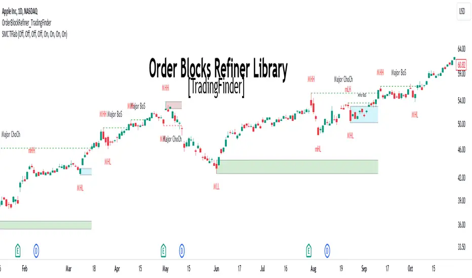
Order Block Refiner [TradingFinder]🔵 Introduction
The "Refinement" feature allows you to adjust the width of the order block according to your strategy. There are two modes, "Aggressive" and "Defensive," in the "Order Block Refine". The difference between "Aggressive" and "Defensive" lies in the width of the order block.
For risk-averse traders, the "Defensive" mode is suitable as it provides a lower loss limit and a greater reward-to-risk ratio. For risk-taking traders, the "Aggressive" mode is more appropriate. These traders prefer to enter trades at higher prices, and this mode, which has a wider order block width, is more suitable for this group of individuals.
Important :
One of the advantages of using this library is increased code accuracy. Not only does it have the capability to create order blocks, but you can also simply define the condition for order block creation (true/false) and "bar_index," and you'll find the primary range without applying any filters.
🟣 Order Block Refinement Algorithm
The order block ranges are filtered in two stages. In the first stage, the "Open," "High," "Low," and "Close" of the current order block candle, its two or three previous candles, and one subsequent candle (if available) are examined. In this stage, minimum and maximum distances are calculated, and logical range filters are applied.
In the second stage, two modes, "Aggressive" and "Defensive," are calculated.
For the "Defensive" mode, the width of these ranges is compared with the "ATR" (Average True Range) of period 55, and if they are smaller than "ATR" or 1 to more than 4 times "ATR," the width of the range is reduced from 0 to 80 percent.
For the "Aggressive" mode, you get the same output as the first filter, which usually has a wider width than the "Defensive" mode.
• Order Block Refiner : Off
• Order Block Refiner : On / "Aggressive Mode"
• Order Block Refiner : On / "Defensive Mode"
🔵 How to Use
OBRefiner(string OBType, string OBRefine, string RefineMethod, bool TriggerCondition, int Index) =>
Parameters:
• OBType (string)
• OBRefine (string)
• RefineMethod (string)
• TriggerCondition (bool)
• Index (int)
To add "Order Block Refiner Library", you must first add the following code to your script.
import TFlab/OrderBlockRefiner_TradingFinder/1
OBType : This parameter receives 2 inputs. If the order block you want to "Refine" is of type demand, you should enter "Demand," and if it's of type supply, you should enter "Supply."
OBRefine : Set to "On" if you want the "Refine" operation to be performed. Otherwise, set to "Off."
RefineMethod : This input receives 2 modes, "Aggressive" and "Defensive." You can switch between these modes according to your needs.
TriggerCondition : Enter the condition with which the order block is formed in this parameter.
Index : Enter the "bar_index" of the candle where the order block is formed in this parameter.
🟣 Function Outputs
This function has 6 outputs: "bar_index" at the beginning of the "Distal" line, "bar_index+1" at the end of the "Distal" line, "Price" at the "Distal" line, "bar_index" at the beginning of the "Proximal" line, "bar_index+1" at the end of the "Proximal" line, and "Price" at the "Proximal" line, which can be used to draw order blocks.
Sample :
= Refiner.OBRefiner('Demand', 'Off', 'Aggressive',BuMChMain_Trigger, BuMChMain_Index)
if BuMChMain_Trigger
BuMChHlineMain := line.new(BuMChMain_Xp1 , BuMChMain_Yp12 , bar_index , BuMChMain_Yp12, color = color.black , style = line.style_dotted)
BuMChLlineMain := line.new(BuMChMain_Xd1 , BuMChMain_Yd12 , bar_index , BuMChMain_Yd12, color = color.black , style = line.style_dotted)
BuMChFilineMain := linefill.new(BuMChHlineMain ,BuMChLlineMain , color = color.rgb(76, 175, 80 , 75 ) )
在脚本中搜索"demand"
Order Blocks Indicator [TradingFinder] Lightning|CHOCH |OB | BOS🔵 Introduction
In "Price Action," an "Order Block" is essentially an area on the price chart where significant players such as institutional traders have executed their moves by placing noteworthy orders. These points often indicate areas where price either attempts to break through (resistance) or returns when it reaches there (support).
Therefore, when discussing the identification of order blocks, we typically refer to finding points where the price has stalled for a while and has accumulated strength before making a significant move in one direction.
Essentially, order blocks assist traders in understanding where large players with "smart money" have likely placed their bulk orders in the market. Traders use these order blocks as part of their overall analysis to identify probable levels where price may change direction.
This version of the order block indicator is designed for traders, adding many indicators to their charts. The minimal design helps minimize disruptions to user focus.
🔵 Identification of Order Blocks
To identify order blocks, first, a "Level Break" must occur. To identify a "Demand Zone," a "High Level Break" is required, and to identify a "Supply Zone," a "Low Level Break" is needed.
Demand Zone :
Supply Zone :
🔵 "Change of Character" or "Market Shift Structure"
"ChoCh" or "MSS" is the "Break Level" that is contrary to the previous trend. For example, if a "Bearish Level" is established in the market and consecutive "Low Levels" are being broken, the price turns upward, breaking a "High Level." This break is called "ChoCh" or "MSS."
🔵 "Break of Structure"
"Break of Structure," or "BoS" for short, is the "Break Level" in the direction of the current trend. For example, if a "Bullish Level" is established in the market, when the price breaks a "High Level," a "BoS" has occurred.
🔵 Features
🟣 Major Level
This feature helps you easily identify major levels. These levels form when the price breaks another major level.
🟣 Refine Order Block
The "Refinement" feature allows you to adjust the width of the order block based on your strategy. There are two modes, "Aggressive" and "Defensive," in Order Block Refine. The difference between "Aggressive" and "Defensive" lies in the width of the order block. For "Risk Averse" traders, the "Defensive" mode is suitable because it provides smaller stop losses and larger reward-to-risk ratios. For "Risk Taker" traders, the "Aggressive" mode is more suitable. These traders prefer to enter trades at higher prices and this mode, where the width of the order block is greater, is more suitable for this group of individuals.
🔵 How to Use
After adding the indicator to your chart, you will see a visual similar to the image below. Green order blocks are "Demand Zones" and red order blocks are "Supply Zones." The midpoint of the order blocks also indicates 50% of it.
Refine Order Block is defaulted to On and refines the order blocks. If you want the order blocks to remain original, you should set it to Off.
Refine is defaulted to "Defensive" mode. If you want it to be in "Aggressive" mode, you should change its mode through Refine Type.
Displaying "Major Levels" is turned off by default and to display them, you should set "Show High Level" and "Show Low Level" to "Yes." You can use these lines to identify liquidity or determine stop loss and take profit levels.

Composite Trend Oscillator [ChartPrime]CODE DUELLO:
Have you ever stopped to wonder what the underlying filters contained within complex algorithms are actually providing for you? Wouldn't it be nice to actually visually inspect for that? Those would require some kind of wild west styled quick draw duel or some comparison method as a proper 'code duello'. Then it can be determined which filter can 'draw' the quickest from it's computational holster with the least amount of lag and smoothness.
In Pine we can do so, discovering how beneficial that would be. This can be accomplished by quickly switching from one filter to another by input() back and forth, requiring visual memory. A better way could be done by placing two indicators added to the chart and then eventually placed into one indicator pane on top of each other.
By adding a filter() helper function that calls other moving average functions chosen for comparison, it can put to the test which moving average is the best drawing filter suited to our expected needs. PhiSmoother was formerly debuted and now it is utilized in a more complex environment in a multitude of ways along side other commonly utilized filters. Now, you the reader, get to judge for yourself...
FILTER VERSATILITY:
Having the capability to adjust between various smoothing methods such as PhiSmoother, TEMA, DEMA, WMA, EMA, and SMA on historical market data within the code provides an advantage. Each of these filter methods offers distinct advantages and hinderances. PhiSmoother stands out often by having superb noise rejection, while also being able to manipulate the fine-tuning of the phase or lag of the indicator, enhancing responsiveness to price movements.
The following are more well-known classic filters. TEMA (Triple Exponential Moving Average) and DEMA (Double Exponential Moving Average) offer reduced transient response times to price changes fluctuations. WMA (Weighted Moving Average) assigns more weight to recent data points, making it particularly useful for reduced lag. EMA (Exponential Moving Average) strikes a balance between responsiveness and computational efficiency, making it a popular choice. SMA (Simple Moving Average) provides a straightforward calculation based on the arithmetic mean of the data. VWMA and RMA have both been excluded for varying reasons, both being unworthy of having explanation here.
By allowing for adjustment refinements between these filter methods, traders may garner the flexibility to adapt their analysis to different market dynamics, optimizing their algorithms for improved decision-making and performance on demand.
INDICATOR INTRODUCTION:
ChartPrime's Composite Trend Oscillator operates as an oscillator based on the concept of a moving average ribbon. It utilizes up to 32 filters with progressively longer periods to assess trend direction and strength. Embedded within this indicator is an alternative view that utilizes the separation of the ribbon filaments to assess volatility. Both versions are excellent candidates for trend and momentum, both offering visualization of polarity, directional coloring, and filter crossings. Anyone who has former experience using RSI or stochastics may have ease of understanding applying this to their chart.
COMPOSITE CLUSTER MODES EXPLAINED:
In Trend Strength mode, the oscillator behavior signifies market direction and movement strength. When the oscillator is rising and above zero, the market is within a bullish phase, and visa versa. If the signal filter crosses the composite trend, this indicates a potential dynamic shift signaling a possible reversal. When the oscillator is teetering on its extremities, the market is more inclined to reverse later.
With Volatility mode, the oscillator undergoes a transformation, displaying an unbounded oscillator driven by market volatility. While it still employs the same scoring mechanism, it is now scaled according to the strength of the market move. This can aid with identification of ranging scenarios. However, one side effect is that the oscillator no longer has minimum or maximum boundaries. This can still be advantageous when considering divergences.
NOTEWORTHY SETTINGS FEATURES:
The following input settings described offer comprehensive control over the indicator's behavior and visualization.
Common Controls:
Price Source Selection - The indicator offers flexibility in choosing the price source for analysis. Traders can select from multiple options.
Composite Cluster Mode - Choose between "Trend Strength" and "Volatility" modes, providing insights into trend directionality or volatility weighting.
Cluster Filter and Length - Selects a filter for the cluster composition. This includes a length parameter adjustment.
Cluster Options:
Cluster Dispersion - Users can adjust the separation between moving averages in the cluster, influencing the sensitivity of the analysis.
Cluster Trimming - By modifying upper and lower trim parameters, traders can adjust the sensitivity of the moving averages within the cluster, enhancing its adaptability.
PostSmooth Filter and Length - Choose a filter to refine the composite cluster's post-smoothing with a length parameter adjustment.
Signal Filter and Length - Users can select a filter for the lagging signal plot, also having a length parameter adjustment.
Transition Easing - Sensitivity adjustment to influence the transition between bullish and bearish colors.
Enjoy

Market Health MonitorThe Market Health Monitor is a comprehensive tool designed to assess and visualize the economic health of a market, providing traders with vital insights into both current and future market conditions. This script integrates a range of critical economic indicators, including unemployment rates, inflation, Federal Reserve funds rates, consumer confidence, and housing market indices, to form a robust understanding of the overall economic landscape.
Drawing on a variety of data sources, the Market Health Monitor employs moving averages over periods of 3, 12, 36, and 120 months, corresponding to quarterly, annual, three-year, and ten-year economic cycles. This selection of timeframes is specifically chosen to capture the nuances of economic movements across different phases, providing a balanced view that is sensitive to both immediate changes and long-term trends.
Key Features:
Economic Indicators Integration: The script synthesizes crucial economic data such as unemployment rates, inflation levels, and housing market trends, offering a multi-dimensional perspective on market health.
Adaptability to Market Conditions: The inclusion of both short-term and long-term moving averages allows the Market Health Monitor to adapt to varying market conditions, making it a versatile tool for different trading strategies.
Oscillator Thresholds for Recession and Growth: The script sets specific thresholds that, when crossed, indicate either potential economic downturns (recessions) or periods of growth (expansions), allowing traders to anticipate and react to changing market conditions proactively.
Color-Coded Visualization: The Market Health Monitor employs a color-coding system for ease of interpretation:
-- A red background signals unhealthy economic conditions, cautioning traders about potential risks.
-- A bright red background indicates a confirmed recession, as declared by the NBER, signaling a critical time for traders to reassess risk exposure.
-- A green background suggests a healthy market with expected economic expansion, pointing towards growth-oriented opportunities.
Comprehensive Market Analysis: By combining various economic indicators, the script offers a holistic view of the market, enabling traders to make well-informed decisions based on a thorough understanding of the economic environment.
Key Criteria and Parameters:
Economic Indicators:
Labor Market: The unemployment rate is a critical indicator of economic health.
High or rising unemployment indicates reduced consumer spending and economic stress.
Inflation: Key for understanding monetary policy and consumer purchasing power.
Persistent high inflation can lead to economic instability, while deflation can signal weak
demand.
Monetary Policy: Reflected by the Federal Reserve funds rate.
Changes in the rate can influence economic activity, borrowing costs, and investor
sentiment.
Consumer Confidence: A predictor of consumer spending and economic activity.
Reflects the public’s perception of the economy
Housing Market: The housing market often leads the economy into recession and recovery.
Weakness here can signal broader economic problems.
Market Data:
Stock Market Indices: Reflect overall investor sentiment and economic
expectations. No gains in a stock market could potentially indicate that economy is
slowing down.
Credit Conditions: Indicated by the tightness of bank lending, signaling risk
perception.
Commodity Insight:
Crude Oil Prices: A proxy for global economic activity.
Indicator Timeframe:
A default monthly timeframe is chosen to align with the release frequency of many economic indicators, offering a balanced view between timely data and avoiding too much noise from short-term fluctuations. Surely, it can be chosen by trader / analyst.
The Market Health Monitor is more than just a trading tool—it's a comprehensive economic guide. It's designed for traders who value an in-depth understanding of the economic climate. By offering insights into both current conditions and future trends, it encourages traders to navigate the markets with confidence, whether through turbulent times or in periods of growth. This tool doesn't just help you follow the market—it helps you understand it.

Volume Heatmap 2024 | NXT2017 Christmas EditionHi big players around the world,
I wish you a merry christmas time.
Today I have a nice present for you: a new volume heatmap indicator for free using!
HISTORY
My first volume heatmap project got a lot of feedback and a big demand. You can find it here:
In this time pinescript version 4 was the newest one and I worked the first time with arrays.
Today we have pinescript version 5 and some new features. This is why I tried again with matrix function and the results are better than I expected.
HOW IT WORKS
The indicator calculates similar like the volume profile. It looks back and every volume where the close price is on the same row area, the volume will cumulated. How much rows the new chart view is showing, you can choose manually.
The mind behind this is to find high volume levels, where high volume catch the price in a range or get function as support/resistance line.
PICTURES
I hope it helps for your trading. You are welcome to give some comments.
Merry christmas and best regards
NXT2017

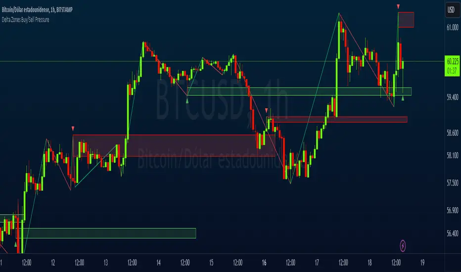
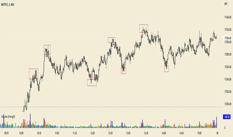
Delta Zones Buy/Sell PressureScript Description:
Delta Zones Buy/Sell Pressure Indicator
Description:
The "Delta Zones Buy/Sell Pressure" indicator, created by the original author "scarf", is a technical tool that unveils key areas of buying and selling pressure in the market. This indicator utilizes the concept of Delta, calculating differences between open, close, high, and low prices. When these differences exceed a threshold determined by the user-defined standard deviation, areas of intense buying (indicated by green boxes) and selling pressure (indicated by red boxes) on the chart are identified.
How It Works:
The indicator calculates Delta using various combinations of candle prices to determine buying and selling pressure. When Delta surpasses a certain level, indicated by the user-defined standard deviation, visual signals in the form of boxes on the chart are generated. These boxes highlight specific areas where buying or selling pressure is particularly strong, aiding traders in identifying potential entry and exit points in the market.
How to Use:
* When a green box is drawn, it indicates strong buying pressure in the market. This can be interpreted as a signal to consider long positions.
* When a red box is drawn, it indicates strong selling pressure in the market. This can be interpreted as a signal to consider short positions.
* Use these signals in combination with your own analysis and risk management strategies to make informed trading decisions.
Originality:
What makes this indicator original is its unique approach to identifying specific areas of buying and selling pressure. By calculating Delta in multiple ways and utilizing standard deviation as a filter, this indicator provides clear and concise visual signals about market activity. The combination of these features distinguishes it as a valuable tool for traders seeking a better understanding of market behavior. This modification differs from the original by displaying the information on the price chart with horizontal bars, below each delta, instead of an oscillator at the bottom similar to the volume indicator.
Final Recommendations:
Consider Market Trends:
Before making any trading decisions using the Delta Zones Buy/Sell Pressure Indicator, it is crucial to analyze the prevailing market trends. Assess the overall direction of the market, whether it's trending upward, downward, or moving sideways. Align your trades with the dominant trend to increase the probability of successful outcomes. The indicator's signals can be more reliable when they align with the broader market trend.
Evaluate Macro-Economic Factors:
Additionally, take into account macro-economic factors that could influence price movements. Factors such as economic indicators, geopolitical events, interest rate decisions, and global market sentiments can significantly impact the financial markets. Stay updated with relevant news and economic reports to anticipate potential market shifts. Understanding the broader economic context can help you interpret the indicator's signals within a more informed framework.
Practice Risk Management:
Regardless of the signals provided by the Delta Zones Buy/Sell Pressure Indicator, always implement effective risk management strategies. This includes setting stop-loss orders, diversifying your portfolio, and only risking a small percentage of your trading capital on each trade. By managing your risk, you can protect your investments and ensure longevity in the market, even during volatile periods.
Continuous Learning and Adaptation:
Financial markets are dynamic and constantly evolving. Continuously educate yourself about new trading strategies, technical analysis tools, and economic developments. Stay open to adapting your trading approach based on changing market conditions. Regularly reviewing your trading strategy and adjusting it according to your experiences and market feedback can significantly enhance your trading performance over the long term.
Seek Professional Advice if Necessary:
If you are uncertain about specific market trends, indicators, or economic factors, don't hesitate to seek guidance from financial advisors or professionals. Their expertise can provide valuable insights and help you make well-informed decisions, especially in complex or uncertain market environments.
By incorporating these recommendations into your trading approach, you can enhance your decision-making process, mitigate risks, and increase your overall chances of successful trading outcomes. Remember, the key to successful trading lies not only in the tools you use but also in your ability to interpret them within the broader market context.
Support & Resistance IndicatorThe MACD Support & Resistance indicator is an enhanced tool to better visualize potential supply (resistance) and demand (support) zones based on the MACD indicator. It combines the strength of the MACD with recent price highs and lows to depict potential breakout or reversal areas in the market.
Features:
MACD Settings: Users can adjust the fast length, slow length, source of MACD, signal smoothing, and MA type for both the oscillator and the signal line.
Dynamic Color Settings: Customize the color of supply boxes, demand boxes, and closed boxes for improved visualization.
Table View: An optional table can be displayed showing the average MACD high and low values, with customizable table position, size, background color, and text color.
Historical MACD Average: The indicator uses a historical average of MACD pivot highs and lows to determine potential support and resistance zones.
Real-Time Zone Detection: The indicator plots 'High Boxes' when the MACD crosses above its average high and 'Low Boxes' when it crosses below its average low, which signifies potential breakout or reversal zones.
How It Works:
The MACD line is calculated using user-defined moving average types (either EMA or SMA).
Pivot highs and pivot lows of the MACD are identified over a specified period.
Historical MACD highs and lows are stored and managed for average calculation. The average MACD high and low values are then used to determine potential trading zones.
When the MACD crosses over its average high, a 'High Box' (representing a potential breakout zone) is plotted from the recent high price to the candle top.
Conversely, when the MACD crosses under its average low, a 'Low Box' (indicating a potential reversal zone) is plotted from the recent low price to the candle base.
As price progresses, the boxes can either extend (if price stays within the zone) or close if a breakout happens.
For those who prefer a tabular view, an optional table displays the average MACD high and low, enhancing the on-chart data representation.
Use Cases:
Traders can use this indicator as an additional tool to spot potential breakout or reversal areas based on the MACD's behavior against its historical average. The visual representation in the form of boxes can assist in making better trading decisions by offering a clear picture of potential supply and demand zones.
Note: As with all trading indicators, it's advisable to use this tool in conjunction with other technical analysis methods or indicators for more informed decision-making.

Psychological Support/Resistence [BigBeluga]The Psychological Support/Resistance indicator aims to provide the user with hypothetical support and resistance zones that are likely to provoke a strong reaction in price, either in both directions, providing good bouncing zones or significant movements once those levels are breached.
🔶 CALCULATION
The script takes into consideration the total number of sequential candles moving in the same direction, as determined by the user's settings. When this sequence is identified, a level is created.
A level is considered broken when the candle's close is above the top/bottom of the level.
Users have the option to select the width of the area based on the Average (AVG), Open, or Close.
AVG will provide the average width of the level of the area.
Close will offer a broader range to work with.
Open will provide a very narrow area.
🔶 METHODOLOGY
The idea behind these areas is that the price will be more likely to produce either a substantial move in the ongoing direction or, when breached, a strong price reaction.
The more the support level is touched or tested, the more likely it is to break.
The longer it has been since its creation and the less it has been tested, the more likely it is to offer strong support or resistance.
Wicks starting to close above the level will indicate a potential breakout to the upside or downside if a candle manages to close above it.
🔶 INPUTS
Users have the option to determine the number of sequential candles.
Users also have the option to decide how many zones to display on the chart.
Color changes are possible.
The possibility to show volume on the creation of the zone is included."

Incomplete Session Candle - Incomplete Timeframe Candle Marker The "Incomplete Session Candle - Incomplete Timeframe Candle Marker" is an advanced tool tailored for technical analysts who understand the importance of accurate timeframes in their charting. While the indicator is not limited to the Indian market, its genesis is rooted in the nuances of trading sessions like those in India, which span 375 minutes from 9:15 AM to 3:30 PM.
Key Features:
Detects if the current timeframe is intraday (minutes or hours).
Calculates the expected duration of the candle for the chosen timeframe.
Highlights candles that don't achieve their expected session duration by placing a cross shape above the bar.
Compatible across various intraday timeframes, aiding traders in spotting discrepancies promptly.
Why We Made This: Not Just for India:
While we looked at the Indian market, this indicator works everywhere. Regular timeframes like 30 minutes, 1 hour, and 2 hours often end with incomplete candles, especially at the end of the trading day. For example:
A 30-minute timeframe makes 13 candles, but the last one is only 15 minutes long.
A 1-hour timeframe shows 7 candles, but the last one is just the last 15 minutes.
By switching to different timeframes like 25 minutes, 75 minutes, and 125 minutes, you get more complete information for better trading decisions. Learn more about this in our article: "Power of 25, 75, and 125-Minute Timeframes in the Indian Market", recognized by Trading View's Editors' Pick.
Benefits:
The indicator extends its benefits even to users without access to certain timeframes. It accommodates traders using a 1-hour timeframe (pertaining to Indian traders). By employing this indicator, traders consistently remain mindful of incomplete candles within their chosen timeframe
For those who utilize concepts like RBR, RBD, DBR, and DBD, this indicator is paramount. An incomplete candle can skew analysis, leading to potential misinterpretations of base or leg candles.
Final thoughts:
In markets like the Indian stock market, adopting such a tool is not just beneficial, but necessary. Whether you have access to unconventional timeframes or are using traditional ones, recognizing and accounting for the limitations of incomplete candles is critical & it's important to know if your candles fit the timeframe properly. This indicator gives you a better view of the market, which helps you make smarter trades.
Lastly, Thank you for your support! Your likes & comments. If you want to give any feedback then you can give in comment section.
Let's conquer the markets together!

Liquidity PeaksThe "Liquidity Peaks" indicator is a tool designed to identify significant supply and demand zones based on volumetric analysis. It analyzes the volume profile within a specified lookback range to pinpoint the most volumetric point and draw corresponding zones on the price chart.
The 𝐋𝐢𝐪. 𝐏𝐞𝐚𝐤𝐬 indicator utilizes volume data to identify key supply and demand areas on the price chart. By examining the volume profile within a defined lookback range, it highlights three distinct zones: liquidity grab, volume containment, and the most volumetric point.
Zones and their meanings:
Liquidity grab (Orange box): This zone represents a price level where there is a significant swipe of the previous demand zone within the volume range. It indicates a potential shift in market sentiment and serves as a key supply or demand area.
Volume containment (Gray box): This zone displays the area of volume contained before the peak in volume. It provides insights into the range where buying or selling pressure was concentrated, highlighting potential support or resistance levels.
Most volumetric point (Light blue box): This zone represents the point within the lookback range that exhibits the highest volume. It signifies a significant area of market interest and indicates a potential supply or demand level.
Adjustable options:
Adjust liquidity Grab: This option allows you to adjust the size of the boxes. When enabled, the box size is set to twice the size of the high or low of the candle's wick. This adjustment enhances the visibility and accuracy of identifying swipes at specific price levels.
Show origin: Enabling this option ensures that the liquidity boxes are drawn from the wick they were created from. This provides a clear visual reference to the specific candle and highlights the liquidity levels associated with it.
Utility:
The 𝐋𝐢𝐪. 𝐏𝐞𝐚𝐤𝐬 indicator is a valuable tool for traders and investors seeking to identify significant supply and demand zones in the market. By analyzing volume data and drawing corresponding zones on the chart, it helps to pinpoint areas where buying or selling pressure is likely to emerge.
Traders can utilize this information to identify potential support and resistance levels, plan their entries and exits, and make more informed trading decisions. The liquidity grab zones can act as potential reversal or breakout points, while the volume containment zones and most volumetric points provide insights into areas of high market interest.
It is important to note that this indicator should be used in conjunction with other technical analysis tools and indicators to confirm trading signals and validate market dynamics.
Example Charts:

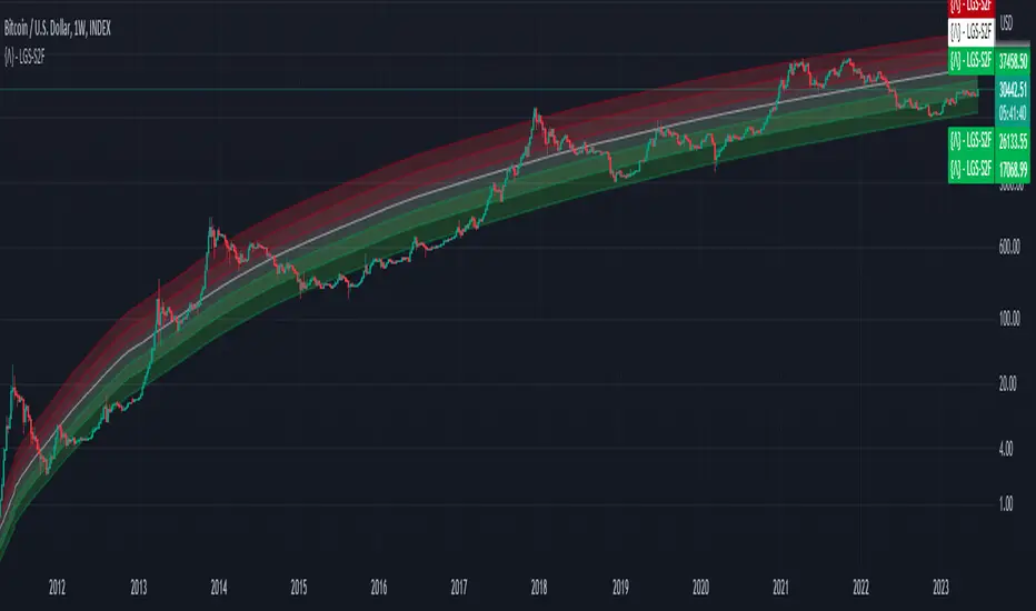
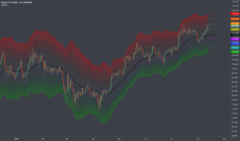
Bitcoin Limited Growth ModelThe Bitcoin Limeted Growth is a model proposed by QuantMario that offers an alternative approach to estimating Bitcoin's price based on the Stock-to-Flow (S2F) ratio. This model takes into account the limitations of the traditional S2F model and introduces refinements to enhance its analysis.
The S2F model is commonly used to analyze Bitcoin's price by considering the scarcity of the asset, measured by the stock (existing supply) relative to the flow (new supply). However, the LGS-S2F Bitcoin Price Formula recognizes the need for improvements and presents an updated perspective on Bitcoin's price dynamics.
Invalidation of the Normal S2F Model:
The normal S2F model has faced criticisms and challenges. One of the limitations is its assumption of a linear relationship between the S2F ratio and Bitcoin's price, overlooking potential nonlinearities and other market dynamics. Additionally, the normal S2F model does not account for external influences, such as market sentiment, regulatory developments, and technological advancements, which can significantly impact Bitcoin's price.
Addressing the Issues:
The LGS-S2F Bitcoin Price Formula introduces refinements to address the limitations of the traditional S2F model. These refinements aim to provide a more comprehensive analysis of Bitcoin's price dynamics:
Nonlinearity: The LGS-S2F model recognizes that the relationship between the S2F ratio and Bitcoin's price may not be linear. It incorporates a logistic growth function that considers the diminishing returns of scarcity and the saturation of market demand.
Data Analysis: The LGS-S2F model employs statistical analysis and data-driven techniques to validate its predictions. It leverages historical data and econometric modeling to support its analysis of Bitcoin's price.
Utility:
The LGS-S2F Bitcoin Price Formula offers insights for traders and investors in the cryptocurrency market. By incorporating a more refined approach to analyzing Bitcoin's price, this model provides an alternative perspective. It allows market participants to consider various factors beyond the S2F ratio alone, potentially aiding in their decision-making processes.
Key Features:
Adjustable Coefficients
Sigma calculation methods: Normal or Stdev
Credit:
The LGS-S2F Bitcoin Price Formula was developed by QuantMario, who has contributed to the field of cryptocurrency analysis through their research and modeling efforts.
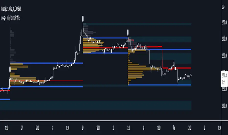
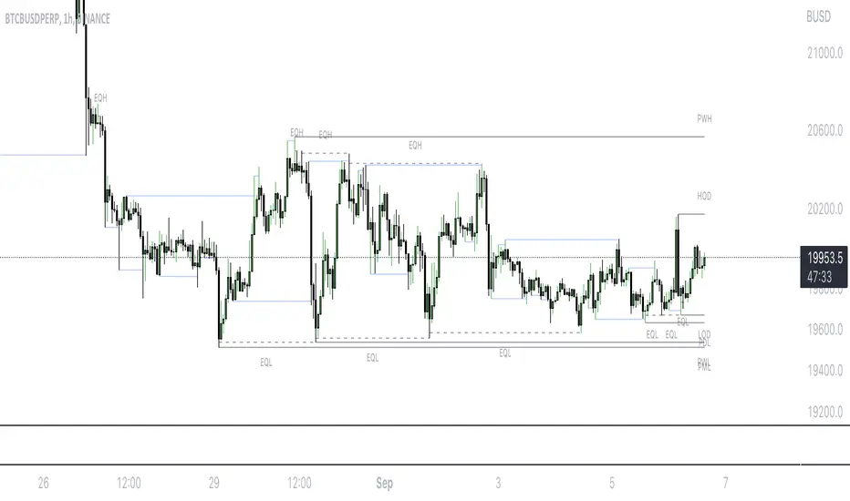
Swing Volume Profiles [LuxAlgo]The Swing Volume Profiles indicator aims to calculate and highlight trading activity at specific price levels between two swing points; allowing traders to reveal dominant and/or significant price levels based on volume.
By measuring traded volume at all price levels in the market over a specified time period, the script can also be used to detect some key analysis generally such as supply & demand, buy-side & sell-side liquidity levels, unfilled liquidity voids, and imbalances that can highlight on the chart.
🔶 USAGE
A volume profile is an advanced charting tool that displays the traded volume at different price levels over a specific period. It helps you visualize where the majority of trading activity has occurred.
Key Levels are the areas where the volume is concentrated or where there are significant volume spikes. These levels are known as key support and resistance levels. High-volume nodes indicate areas of high activity and are likely to act as support or resistance in the future.
Volume profile also helps identify value areas, which represent the price levels where the most trading activity has taken place. These levels can act as areas of support or resistance as traders perceive them as fair value.
The Point of Control describes the price level where the most volume was traded. A Naked Point of Control (also called a Virgin Point of Control) is a previous POC that has not been traded. Extending PoC options 'Until Bar Cross' or 'Until Bar Touch' helps in identifying Naked Point of Control Lines.
Previous PoC levels can serve as support and resistance for future price movements. Extending PoC Level 'Until Last Bar' option will help to identify such levels.
🔶 DETAILS
One of the unique features of the script is its ability to detect some other key levels such as levels of acceptance and rejection.
Levels of rejection we may summarize as supply and demand levels, these are also referred to as buy-side and sell-side liquidity levels. They usually occur at extreme highs or lows, where prices may be too high for buyers (high supply, low demand) or too low for sellers (low supply, high demand)
Levels of acceptance are the levels where Liquidity Voids occur, these are also referred to imbalances. Liquidity voids are sudden changes in price when the price jumps from one level to another. The peculiar thing about liquidity voids is that they almost always fill up, so we call them levels of acceptance.
🔶 ALERTS
When an alert is configured, the user will have the ability to be notified in case:
Point Of Control Line is touched/crossed
Value Area High Line is touched/crossed
Value Area Low Line is touched/crossed
🔶 SETTINGS
🔹 Display Options
Mode: Controls the lookback length of detection and visualization, where Present assumes last X bars specifid in '# Bars' option and Historical assumes all data available to the user as well as allowed limits of visiual objects (boxs, lines, labels etc)
# Bars: Controls the lookback length.
🔹 Swing Volume Profiles
The script takes into account user-defined parameters and plots volume profiles. Due to Pine Script™ drwaing objects limit only total volume profiles are presented.
Swing Detection Length: Lookback period
Swing Volume Profiles: Toggles the visibility of the Volume Profiles, with color options to differentiate the Value Area within a profile.
Profile Range Background Fill: Toggles the visibility of the Volume Profiles Range
🔹 Point of Control (PoC)
Point of Control (POC) – The price level for the time period with the highest traded volume
Point of Control (PoC): Toggles the visibility of the Point of Control
Developing PoC: Toggles the visibility of the Developing PoC
Extend PoC: Option that allows detecting virgin PoC levels. Virgin Point of Control (VPoC) is defined as a Point of Control that has never been revisited or touched. The option also allows PoC levels to extend till the last bar aiming to present levels from history where the levels were traded significantly and those levels can be used as support and resistance levels.
🔹 Value Area (VA)
Value Area (VA) – The range of price levels in which the specified percentage of all volume was traded during the time period.
Value Area Volume %: Specifies percentage of the Value Area
Value Area High (VAH): Toggles the visibility of the Value Area High, the highest price level within the Value Area
Value Area Low (VAL): Toggles the visibility of the Value Area Low, the lowest price level within the Value Area
Value Area (VA) Background Fill: Toggles the visibility of the Value Area Range
🔹 Liquidity Levels / Voids
Unfilled Liquidity, Thresh: Enable display of the Unfilled Liquidity Levels and Liquidity Voids, where threshold value defines the significance of the level.
🔹 Profile Stats
Position, Size: Specifies the position and the size of the label presenting Profile Stats, the tooltip of the label includes all related info for each profile.
Price, Price Change, and Cumulative Volume: Enable display of the given options on the chart.
🔹 Volume Profile Others
Number of Rows: Specify how many rows each histogram will have. Caution, having it set to high values will quickly hit Pine Script™ drawing objects limit and may cause fewer historical profiles to be displayed.
Placement: Place profile either left or right.
Profile Width %: Alters the width of the rows in the histogram, relative to the calculated profile length.
🔶 RELATED SCRIPTS
Alternative Liquidity Void Detection script, Buyside-Sellside-Liquidity
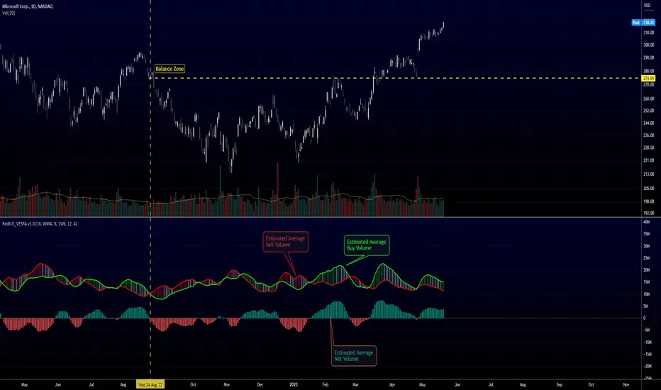
Directional Volume EStimate from Price Action (RedK D_VESPA)The "Directional Volume EStimate from Price Action (RedK D_VESPA)" is another weapon for the VPA (Volume Price Analysis) enthusiasts and traders who like to include volume-based insights & signals to their trading. The basic concept is to estimate the sell and buy split of the traded volume by extrapolating the price action represented by the shape of the associated price bar. We then create and plot an average of these "estimated buy & sell volumes" - the estimated average Net Volume is the balance between these 2 averages.
D_VESPA uses clear visualizations to represent the outcomes in a less distracting and more actionable way.
How does D_VESPA work?
-------------------------------------
The key assumption is that when price moves up, this is caused by "buy" volume (or increasing demand), and when the price moves down, this is due to "selling" volume (or increasing supply). Important to note that we are making our Buy/sell volume estimates here based on the shape of the price bar, and not looking into lower time frame volume data - This is a different approach and is still aligned to the key concepts of VPA.
Originally this work started as an improvement to my Supply/Demand Volume Viewer (V.Viewer) , I ended up re-writing the whole thing after some more research and work on VPA, to improve the estimation, visualization and usability / tradability.
Think of D_VESPA as the "Pro" version of V.Viewer -- and please go back and review the details of V.Viewer as the root concepts are the same so I won't repeat them here (as it comes to exploring Balance Zone and finding Price Convergence/Divergence)
Main Features of D_VESPA
--------------------------------------
- Update Supply/Demand calculation to include 2-bar gaps (improved algo)
- Add multiple options for the moving average (MA type) for the calculation - my preference is to use WMA
- Add option to show Net Volume as 3-color bars
- Visual simplification and improvements to be less distracting & more actionable
- added options to display/hide main visuals while maintaining the status line consistency (Avg Supply, Avg Demand, Avg Net)
- add alerts for NetVol moving into Buy (crosses 0 up) or Sell (crosses 0 down) modes - or swing from one mode to the other
(there are actually 2 sets of alerts, one set for the main NetVol plot, and the other for the secondary TF NetVol - give user more options on how to utilize D_VESPA)
Quick techie piece, how does the estimated buy/sell volume algo work ?
------------------------------------------------------------------------------------------
* per our assumption, buy volume is associated with price up-moves, sell volume is associated with price down-moves
* so each of the bulls and bears will get the equivalent of the top & bottom wicks,
* for up bars, bulls get the value of the "body", else the bears get the "body"
* open gaps are allocated to bulls or bears depending on the gap direction
The below sketch explains how D_VESPA estimates the Buy/Sell Volume split based on the bar shape (including gap) - the example shows a bullish bar with an opening gap up - but the concept is the same for a down-bar or a down-gap.
I kept both the "Volume Weighted" and "2-bar Gap Impact" as options in the indicator settings - these 2 options should be always kept selected. They are there for those who would like to experiment with the difference these changes have on the buy/sell estimation. The indicator will handle cases where there is no volume data for the selected symbol, and in that case, it will simply reflect Average Estimated Bull/Bear ratio of the price bar
The Secondary TF Est Average Net Volume:
---------------------------------------------------------
I added the ability to plot the Estimate Average Net Volume for a secondary timeframe - options 1W, 1D, 1H, or Same as Chart.
- this feature provides traders the confidence to trade the lower timeframes in the same direction as the prevailing "market mode"
- this also adds more MTF support beyond the existing TradingView's built-in MTF support capability - experiment with various settings between exposing the indicator's secondary TF plot, and changing the TF option in the indicator settings.
Note on the secondary TF NetVol plot:
- the secondary TF needs to be set to same as or higher TF than the chart's TF - if not, a warning sign would show and the plot will not be enabled. for example, a day trader may set the secondary TF to 1Hr or 1Day, while looking at 5min or 15min chart. A swing/trend trader who frequently uses the daily chart may set the secondary TF to weekly, and so on..
- the secondary TF NetVol plot is hidden by default and needs to be exposed thru the indicator settings.
the below chart shows D_VESPA on a the same (daily) chart, but with secondary TF plot for the weekly TF enabled
Final Thoughts
-------------------
* RedK D_VESPA is a volume indicator, that estimates buy/sell and net volume averages based on the price action reflected by the shape of the price bars - this can provide more insight on volume compared to the classic volume/VolAverage indicator and assist traders in exploring the market mode (buyers/sellers - bullish/bearish) and align trades to it.
* Because D_VESPA is a volume indicator, it can't be used alone to generate a trading signal - and needs to be combined with other indicators that analysis price value (range), momentum and trend. I recommend to at least combine D_VESPA with a variant of MACD and RSI to get a full view of the price action relative to the prevailing market and the broader trend.
* I found it very useful to take note and "read" how the Est Buy vs Est Sell lines move .. they sort of "tell a story" - experiment with this on your various chart and note the levels of estimate avg demand vs estimate avg supply that this indicator exposes for some very valuable insight about how the chart action is progressing. Please feel free to share feedback below.
ICT Implied Fair Value Gap (IFVG) [LuxAlgo]An Implied Fair Value Gap (IFVG) is a three candles imbalance formation conceptualized by ICT that is based on detecting a larger candle body & then measuring the average between the two adjacent candle shadows.
This indicator automatically detects this imbalance formation on your charts and can be extended by a user set number of bars.
The IFVG average can also be extended until a new respective IFVG is detected, serving as a support/resistance line.
Alerts for the detection of bullish/bearish IFVG's are also included in this script.
🔶 SETTINGS
Shadow Threshold %: Threshold percentage used to filter out IFVG's with low adjacent candles shadows.
IFVG Extension: Number of bars used to extend highlighted IFVG's areas.
Extend Averages: Extend IFVG's averages up to a new detected respective IFVG.
🔶 USAGE
Users of this indicator can primarily find it useful for trading imbalances just as they would for trading regular Fair Value Gaps or other imbalances, which aims to highlight a disparity between supply & demand.
For trading a bullish IFVG, users can find this imbalance as an area where price is likely to fill or act as an area of support.
In the same way, a user could trade bearish IFVGs by seeing it as a potential area to be filled or act as resistance within a downtrend.
Users can also extend the IFVG averages and use them as longer-term support/resistances levels. This can highlight the ability of detected IFVG to provide longer term significant support and resistance levels.
🔶 DETAILS
Various methods have been proposed for the detection of regular FVG's, and as such it would not be uncommon to see various methods for the implied version.
We propose the following identification rules for the algorithmic detection of IFVG's:
🔹 Bullish
Central candle body is larger than the body of the adjacent candles.
Current price low is higher than high price two bars ago.
Current candle lower shadow makes up more than p percent of its total candle range.
Candle upper shadow two bars ago makes up more than p percent of its total candle range.
The average of the current candle lower shadow is greater than the average of the candle upper shadow two bars ago.
where p is the user set threshold.
🔹 Bearish
Central candle body is larger than the body of the adjacent candles.
Current price high is higher than low price two bars ago.
Current candle upper shadow makes up more than p percent of its total candle range.
Candle lower shadow two bars ago makes up more than p percent of its total candle range.
The average of the candle lower shadow 2 bars ago is greater than the average of the current candle higher shadow.
where p is the user set threshold.
🔶 SUPPLEMENTARY MATERIAL
You can see our previously posted script that detects various imbalances as well as regular Fair Value Gaps which have very similar usability to Implied Fair Value Gaps here:

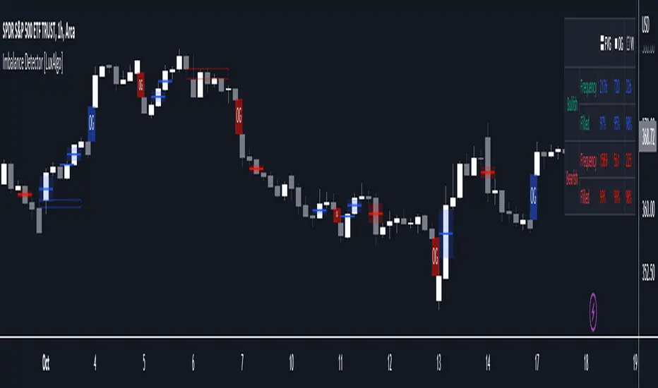
Imbalance Detector [LuxAlgo]This indicator detects and highlights market imbalances alongside a dashboard returning information about their frequency of occurrence and their fill percentage. Imbalances included in this script are Fair Value Gaps (FVG), Opening Gaps (OG) and Volume Imbalances (VI).
Alerts are available for the occurrences of all market imbalances.
Settings
Imbalances
Each imbalance has the same settings layout:
Imbalance: Enable/disable the detection of the specific imbalance.
Min Width: If enabled, requires the imbalance area width to be greater than the specified value. This minimum width can be expressed in points, percentages or ATR multiples.
Extend: Extend imbalances by a specified number of bars.
Dashboard
Show Dashboard: Enable/disable the dashboard on the chart.
Dashboard Location: Location of the dashboard on the chart.
Dashboard Size: Size of the dashboard.
Usage
Market imbalances are part of the many concepts available to price action traders and highlight areas where there is a disparity between supply and demand.
It is common to see price come back to these areas and traders often use them as supports and resistances but also as targets.
Details
The script can detect three distinct types of imbalances described below.
Fair Value Gaps
Fair Value Gaps (FVG) are three candle formations characterized by a gap between the wicks of the non-adjacent candles in the formation.
A bullish FVG is characterized by a gap between the current price low and the 2 bars anterior price high, and a bearish FVG is characterized by a gap between the current price high and the 2 bars anterior price low.
Opening Gaps
Opening Gaps (OG) are imbalances characterized by non-existent activity within a specific price range.
A bullish OG occurs when the current price low is greater than the previous high, a bearish OG occurs when price high is lower than the previous price low.
Opening Gaps primarily occur in closing markets, as such they are less common in the cryptocurrency market.
Most of the time an Opening Gap will also be accompanied by a Fair Value Gap, in order to avoid clutter the indicator will not detect Fair Value Gaps if Opening Gaps are enabled and if an Opening Gap has been detected
Volume Imbalances
Volume Imbalances (VI) are characterized by a price discontinuity between the opening price and previous close, but unlike Opening Gaps we do not see nonexistent activity within a certain price range.
A bullish VI occur when both the opening and closing prices are superior to the previous closing price, with the current price low overlapping the previous price high. A bearish VI occur when both the opening and closing prices are inferior to the previous closing price, with the current price high overlapping the previous price low.
Because Volume Imbalances can occur excessively on markets with frequent gaps, we make use of an additional condition for filtering out less significant imbalances. Bullish VI's will require the previous price high to be lower than the opening price, while bullish VI's will require the previous price low to be higher than the opening price.
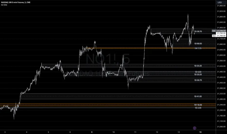
Gap ZonesSharing a simple gap zone identifier, simply detects gap up/down areas and plots them for visual reference. Calculation uses new candle open compared to previous candle close and draws the zone, a mid point is plotted also as far too often it's significance is proven effective.
Works on any timeframe and market though I recommend utilizing timeframes such as weekly or daily for viewing at lower timeframes such as 5, 15 or 30 minutes.
Often price is observed reaching towards zone high/mid/low before rejection/bouncing. These gap zones can give quantitative basis for trade management.
Future features may include alerts based on price crossing up/down gap low, mid and highs. Feel free to message with any other suggestions.
Volume HIGH/CLIMAX
Volume is the number of shares of a security traded during a given period of time.
Generally securities with more daily volume are more liquid than those without, since they are more "active".
Volume is an important indicator in technical analysis because it is used to measure the relative significance of a market move.
The higher the volume during a price move, the more significant the move and the lower the volume during a price move, the less significant the move.
A climax occurs at the end of a bull or bear market cycle and is characterized by escalated trading volume and sharp price movements.
Climaxes are usually preceded by extreme sentiment readings, either excessive euphoria at market peaks, or excessive pessimism at market bottoms.
Essentially, climaxes are a result of a resolution in supply and demand factors.
Buying Climaxes
One of the clearest signals of the end of a bull market is a buying climax, during which volume escalates to extreme levels and bullish euphoria permeates media coverage of stocks, market indices, or commodities . The key trait of a buying climax is the exhaustion of demand as the last buyers enter the market. The final surge of buying typically leads to price spikes, which may last for days, weeks, or months. As demand wanes, buyers become less willing to pay higher prices. There may be a brief period of stagnation in prices before a combination of profit-taking and new sellers set in motion the start of a sharp reversal.
Selling Climaxes
The beginning of a selling climax is often signaled by steadily increasing volume on the sell side of the market as growing pessimism accelerates the downtrend. As the selling climax approaches, the last buyers finally capitulate, driving shares sharply lower. Once the supply side of the market abates, demand at support levels can cause the price to level off before a combination of profit-taking and new buyers set in motion the start of a sharp reversal.
Nonlinear Parametric Oscillator - PSOThis script is in development phase and may be buggy. use with your own risk. The idea here is to determine the sinusoidal directional changes in the supply and demand. Based on direction, you can enter and make huge gains. Recommended to use on 1 min chart. The sideways market would be indicated as flattening in the respective bands. There are four bands, bottom one is where market is in BEAR mode and top one is when market is in BULL mode.
The indicator doesnt work well when the ticker price is less than 10 dollars, i am working on it. Do not use on penny stocks, for the time. More-details when I make this a robust version.

Price Action in action
What?
Price Action in Action is an indicator to help Price Action learners and practitioners to get everything related for Price Action in one place.
Price Action is:
Price + Volume = Action
In this indicator, we have the following features available:
Support/Resistance
Using the RSI with different periods in a multiple of 7 (7, 14, 21, 28), we first determine the overbought (above 70, customizable) and oversold (below 30, customizable) regions. Then we pick up the highest point and lowest point in the RSI values in the overbought and oversold regions, respectively. These are the point, historically supply/demand emerged for surety to push down/up the RSI indicator and the corresponding price. So, these are the most accurate way, we believe, to draw support/resistance (or demand/supply) in the chart. By default, the Support is green color and Resistance is red color. To give a visual representation, we differentiate the different shades of green and red. For example, for Level-1 (i.e. 7 by default) we use the darkest shade (0 transparency) and Level-4 (i.e. 28 by default) we use lighter shade (60 transparency). Note please: you can customize the color of support and resistance lines (say if you want resistance as green and support as red). The respective shades (transparency) will be automatically adjusted accordingly. But those shade (transparency) levels are not customizable, they are fixed (please bear with it for version-1 at least).
Strength of Support/Resistance
In the chart above/below the Resistance / Support lines you can see the tiny labels with some numbers like 1, 2.
We found out how many times a particular support/resistance is appearing across multiple RSI periods. E.g. if price P1 appears 2 times among 4 different RSI periods, the number will be 2 for that calculation, and so on.
There can be multiple presence of these numbers in a support/resistance line (i.e. multiple tiny labels). Something like: 1, 1, 2 (into different candles). This means the same support/resistance is tested so many times in different occasion (means there is a RSI max/min coincides in this level over multiple occasions) at different candles.
This will help you to intuitionally gauge the “strength” of a support/resistance line.
The more the marrier, unworthy to mention.
Candle Stick Patterns
Well: we don’t need to tell anything about the Candlestick. All of you know it better than us. And it’s a time proven, zero-lag mechanism to judge the Price-Action is unfolding in the market. We do not know if there is anything better possible than this time tested patterns to judge the prevailing sentiments of market.
Price-Action does not complete without finding out the Candlestick Patterns correctly.
And in this indicator your will get all of these: Single Candle such as Doji (default off), Marubozu, Spinner, hammers, inverted-hammer etc. ; 2 candles like Tweezer, Inside Candle, Engulfing; 3 candles like morning star/evening star.
In the multi candle patterns (2/3 candles), we are grouping the candles with a dotted rectangle such that it is clear which 2/3 candles are part of the pattern. E.g. Morning Star: 3 candles are grouped in a dotted rectangle and the Morning Star label will come to the latest candle (3rd most – as the pattern is detected reliably only on the completion of the 3rd final candle).
Of course, any program can not eliminate your trained eyes and brain to capture the patterns. But we have provided sufficient knobs to adjust various parameters to tweak the candle-pattern detection. Such as Strict Inside Candle(Harami) Boolean knob where the whole current candle including wicks will be inside the body part of the previous big candle. For non-strict mode, the current candle just inside the previous candle, possibly by wicks.
To make it better usable, for every such knobs (which are not obvious) we have added user-friendly tooltip (just mouse hover the question mark (?) besides the control/switch). There are plenty of it.
Volume
Here we have a rudimentary (yet effective) way to judge the volumes.
We find out the Volume Weighted Moving Average (VMWA) of the 20-period (default, but customizable) and the latest volume. If the latest volume is more than the 20 period vwma, we just add a grey diamond on the top of the candle to denote it’s attracting volumes. Of course, we provide a Weight coefficient (default is set to 1). So if the current bar’s volume on bar’s completion is more than the 20 period volume vmwa times the weigh-cofficient, we mark it with a tiny grey diamond.
Points to be noted:
In all places we mark the indication only on the completion of the bar (technically speaking we have checks, as far as possible, with barstate.isconfirmed). However, if you wish, you can turn it off for Candlestick (as some experts may want to check candlestick on the real time, even before the closing of bars).
In case if you see the chart looks cluttered (because of many information, specially in smaller timeframes like 5 min), there are controls given in the settings to toggle each and every features.
By default, we turn off Doji candles (all 3 types of Doji’s – normal, Gravestone & Dragonfly) as they are mainly indecision. However, you can toggle it to turn it on.
It does not give you any Buy/Sell call. The interpretation it does not have.
Why?
What’s unique in it?
As we already mentioned our intention is to include Price (in forms of Support / Resistance), Volume and Action (sentiments in terms of Candlestick patterns) into a single place. And so far, to the best of our knowledge, we could not come across a single indicator provides all of these.
There were works available to determine the RSI based support / resistance zones. Those are great piece works at that time (lets say 3 years back when PineScript was in earlier versions). To the best of our knowledge those does not cover up finding out the lowest / highest point of RSI and the corresponding price to get the simplistic and distinct support/resistance lines.
We have the intuitive support/resistance strength included which we could not found out in current set of available indicators.
To the best of our knowledge, there seems no indicator can detect 3-candle patterns which are extremely popular to detect trend reversals (such as Morning Star or Evening Star). Moreover for the multi-candle patterns we are grouping the candles part of the pattens (2-candles or 3-candles) using a dotted rectangle such that it’s visually clearly (and a well educative material for Price-Action learners also).
Mentions:
There are many works which inspire us along the way. Honestly: we sometimes forgot which all indicators we experimented with. We are sincerely apologetic in case we forgot to mention. A few note-worthy:
There is an indicator from user “repo32” named as “Candlestick Patterns Identified (updated 3/11/15)”. (We could not be able to contact “repo32”). We are inspired from his work that it’s feasible to detect Candlestick patterns.
There is an awesome work done by “RSI Based Automatic Demand and Supply” by user “shtcoinr”. The idea of consulting multiple RSI levels to find out the demand/supply zone we inspired from him. (We did contact “shtcoinr” and got his kind permission to use the concept.)
We are greatly thankful to these abovementioned wizards for their pioneering a-prior work in this front.
And of course, this TradingView platform to provide this abstraction, facilitates and felicitates collaborative contributions.
Ultimately, what’s for you?
That’s the main question. What’s for you?
Price-action comprises of following 3 tasks (at least):
Draw support/resistance lines in the chart.
Once price reaches at the support/resistance line, you fervently look out the candles’ formation to mentally map to the candle patterns. Your aim is divine: You want to judge if the price-action will continue or take a rejection/reversal.
Then you double-confirm with the volume (in a non-overlaid chart below).
Finally take a trade.
For a price-action newbie or seasoned, expert practitioner, you must be doing all the above tasks regularly and manually, in a mechanical, mundane way. There come the humanly subjectivity & the inevitable emotions . This indicator, being a piece of program/code in PineScript latest version v5 , eliminates (or at least, reduces to a great extend) that subjectivity & emotions out of the way of decision making . Thus resulting better yield.
Of course, you can argue that you draw slanted trend lines also. We recommend an already existing indicator by user LuxAlgo named as “Trendlines with Breaks ”, if you wish so.
Disclaimer:
This piece of software does not come up with any warrantee or any rights of not changing it over the future course of time.
We are not responsible for any trading/investment decision you are taking out of the outcome of this indicator.
Happy trading.

Mark LevelsMark Levels is marking liquidity pools by drawing lines on their pivots and labelling them so that you can instantly detect them on your realtime chart
It supports:
- marking previous and current day lows and highs
- marking previous and current week lows and highs
- marking previous and current month lows and highs
- marking equal lows and highs
technically it re-builds them on the last bar or as soon as new realtime bar is updated. it looks with 1k bars back to find higher timeframe ranges and find lows and highs there
Adjustments:
- changing the line style of the group
- changing the lines color and the labels on the groups
- currently pools are split on 2 groups Period Liquidity and Equal Pivots Liquidity.
Refracted EMARefracted EMA is a price based indicator with bands that is built on moving average.
The price range between the bands directly depends on relationship of Average True Range to Moving Average. This gives us very valuable variable constant that changes with the market moves.
So the bands expand and contract due to changes in volatility of the market, which makes this tool very flexible exposing psychological levels.
Customizable Pivot Support/Resistance Zones [MyTradingCoder]This script uses the standard pivot-high/pivot-low built-in methods to identify pivot points on the chart as a base calculation for the zones. Rather than displaying basic lines, it displays a zone from the original pivot point to the closest part of the available body on the same candle. The script comes in handy by utilizing Pinescripts available input.source() function to allow for an external indicators output value to be used within the indicator. Make sure to read all of the TOOLTIPS in the indicator settings menu to get a full understanding of what each setting does, and how it can affect the results that end up on the chart.
By enabling the custom filter in the indicator settings, you will notice you have the ability to filter out zones using an external indicator such as an RSI. Maybe you only want zones to be calculated/drawn when the RSI is overbought or oversold, or maybe you only want the zones to calculate/draw if the Supertrend is green or red. The list of possible filters that you can implement is too many to count. Feel free to play around with the indicator however you like, and configure something that you find to be the most useful for your trading.
On top of everything listed above, the indicator has pre-programmed built-in alertconditions so that you can potentially automate trading, or get a notification to your cell phone when a zone is being touched/broken.

The Investment ClockThe Investment Clock was most likely introduced to the general public in a research paper distributed by Merrill Lynch. It’s a simple yet useful framework for understanding the various stages of the US economic cycle and which asset classes perform best in each stage.
The Investment Clock splits the business cycle into four phases, where each phase is comprised of the orientation of growth and inflation relative to their sustainable levels:
Reflation phase (6:01 to 8:59): Growth is sluggish and inflation is low. This phase occurs during the heart of a bear market. The economy is plagued by excess capacity and falling demand. This keeps commodity prices low and pulls down inflation. The yield curve steepens as the central bank lowers short-term rates in an attempt to stimulate growth and inflation. Bonds are the best asset class in this phase.
Recovery phase (9:01 to 11:59): The central bank’s easing takes effect and begins driving growth to above the trend rate. Though growth picks up, inflation remains low because there’s still excess capacity. Rising growth and low inflation are the Goldilocks phase of every cycle. Stocks are the best asset class in this phase.
Overheat phase(12:01 to 2:59): Productivity growth slows and the GDP gap closes causing the economy to bump up against supply constraints. This causes inflation to rise. Rising inflation spurs the central banks to hike rates. As a result, the yield curve begins flattening. With high growth and high inflation, stocks still perform but not as well as in recovery. Volatility returns as bond yields rise and stocks compete with higher yields for capital flows. In this phase, commodities are the best asset class.
Stagflation phase (3:01 to 5:59): GDP growth slows but inflation remains high (sidenote: most bear markets are preceded by a 100%+ increase in the price of oil which drives inflation up and causes central banks to tighten). Productivity dives and a wage-price spiral develops as companies raise prices to protect compressing margins. This goes on until there’s a steep rise in unemployment which breaks the cycle. Central banks keep rates high until they reign in inflation. This causes the yield curve to invert. During this phase, cash is the best asset.
Additional notes from Merrill Lynch:
Cyclicality: When growth is accelerating (12 o'clock), Stocks and Commodities do well. Cyclical sectors like Tech or Steel outperform. When growth is slowing (6 o'clock), Bonds, Cash, and defensives outperform.
Duration: When inflation is falling (9 o'clock), discount rates drop and financial assets do well. Investors pay up for long duration Growth stocks. When inflation is rising (3 o'clock), real assets like Commodities and Cash do best. Pricing power is plentiful and short-duration Value stocks outperform.
Interest Rate-Sensitives: Banks and Consumer Discretionary stocks are interest-rate sensitive “early cycle” performers, doing best in Reflation and Recovery when central banks are easing and growth is starting to recover.
Asset Plays: Some sectors are linked to the performance of an underlying asset. Insurance stocks and Investment Banks are often bond or equity price sensitive, doing well in the Reflation or Recovery phases. Mining stocks are metal price-sensitive, doing well during an Overheat.
About the indicator:
This indicator suggests iShares ETFs for sector rotation analysis. There are likely other ETFs to consider which have lower fees and are outperforming their sector peers.
You may get errors if your chart is set to a different timeframe & ticker other than 1d for symbol/tickers GDPC1 or CPILFESL.
Investment Clock settings are based on a "sustainable level" of growth and inflation, which are each slightly subjective depending on the economist and probably have changed since the last time this indicator was updated. Hence, the sustainable levels are customizable in the settings. When I was formally educated I was trained to use average CPI of 3.1% for financial planning purposes, the default for the indicator is 2.5%, and the Medium article backtested and optimized a 2% sustainable inflation rate. Again, user-defined sustainable growth and rates are slightly subjective and will affect results.
I have not been trained or even had much experience with MetaTrader code, which is how this indicator was originally coded. See the original Medium article that inspired this indicator if you want to audit & compare code.
Hover over info panel for detailed information.
Features: Advanced info panel that performs Investment Clock analysis and offers additional hover info such as sector rotation suggestions. Customizable sustainable levels, growth input, and inflation input. Phase background coloring.
⚠ DISCLAIMER: Not financial advice. Not a trading system. DYOR. I am not affiliated with Medium, Macro Ops, iShares, or Merrill Lynch.
About the Author: I am a patent-holding inventor, a futures trader, a hobby PineScripter, and a former FINRA Registered Representative.