Gann Octave Pro - Angles & Time Cycles 🎯 Gann Octave Pro - Angles & Time Cycles
## Complete Gann Trading System - Price, Angles & Time in One Indicator
A professional-grade Gann analysis tool combining **Octave Price Levels**, **Gann Angles (1x1, 2x1, 1x2)**, and **Advanced Time Cycle Projections**. Perfect for traders seeking precision market timing through geometric confluence.
---
## 🌟 Key Features
### 📐 Octave Price Levels
- **5 Key Levels**: 0%, 25%, 50%, 75%, 100%
- **Color-Coded**: Green (support) → Blue (50% pivot) → Red (resistance) → Black (boundaries)
- **Dynamic Updates**: Auto-adjusts to swing structure
- **Trading Edge**: 50% level is the most powerful reversal zone
### 📏 Gann Angles
- **1x1 Angle** (Black) - Natural 45° trend line
- **2x1 Angle** (Red) - Steep acceleration zone
- **1x2 Angle** (Red) - Gradual support/resistance
- **Customizable Extension**: Fixed bars or % of swing length
### ⏰ Advanced Time Cycles
**Three Calculation Methods:**
1. **Angle-Level Confluence** ⭐ (Recommended)
- Calculates intersections of Gann angles with octave levels
- Most sophisticated timing system
- Based on price-time geometry
2. **Swing Duration** - Uses actual swing bar length
3. **Harmonic (Swing/8)** - Classic Gann harmonic division
**Cycle Visualization:**
- **Full Cycles** (Purple, solid) - Major turning points, labeled "◆ FC1 (176 bars) "
- **Sub-Cycles** (Blue, dotted) - Minor pivots, labeled "S1 "
- **Mid-Cycles** (Orange, dashed) - Half-cycle inflection points
- **Past Display**: Shows 4 complete past cycles for validation
- **Future Projection**: Projects 8 future cycles for anticipation
---
## 🎯 How to Use
### Quick Start
1. Apply to chart (works all timeframes/instruments)
2. Select period: Default 44 bars (adjust based on timeframe)
3. Choose cycle method: "Angle-Level Confluence" for best results
4. Observe past cycles to validate timing accuracy
### Trading Strategies
**Triple Confluence Setup** (Highest Probability)
- Price at octave level (especially 50%)
- Price touches Gann angle (1x1 most reliable)
- Time cycle arrives (full cycle preferred)
- **Entry**: On confluence | **Stop**: Below/above octave level | **Target**: Next level
**Cycle Anticipation**
- Enter 1-2 bars before cycle line if price at octave level
- Exit at next cycle or target octave level
- **Edge**: Anticipate cycles instead of reacting
**Angle Breakout + Cycle**
- Price breaks 1x1 angle + next cycle within 20 bars
- Hold through cycle, exit at 2x1 angle or next major level
---
## ⚙️ Customization
### Period Selection (88-Based)
11 harmonic options: 3, 6, 11, 22, **44**, 88, 176, 352, 704, 1408, 2816 bars
- **Intraday** (15m-1h): Period 3-4
- **Swing Trading** (4h-Daily): Period 4-5
- **Position Trading** (Daily-Weekly): Period 5-6
### Visual Controls
- **Colors**: Independent for all elements
- **Line Widths**: Separate controls (1-5) for levels, angles, cycles
- **Label Size**: Tiny/Small/Normal/Large (unified)
- **Label Position**: Top/Middle/Bottom
- **Show/Hide**: Toggle any component
### Alerts
- 50% octave level breakouts
- Customizable messages
---
## 💡 Pro Tips
1. **Validate First**: Observe 2-3 past cycles before trading
2. **Adjust to Volatility**: High volatility = lower period (22-44), Low = higher (88-176)
3. **Multiple Timeframes**: Apply on different timeframes for confirmation
4. **Respect 50% Level**: Most powerful reversal zone in Gann theory
5. **Focus on Full Cycles**: Highest probability setups (◆ FC markers)
6. **Combine with Price Action**: Indicator shows WHERE/WHEN, price action shows HOW
---
## 🚀 What Makes It Unique
✅ **Intelligent Confluence Cycles** - Unique angle-level intersection calculation
✅ **Historical Validation** - See past cycles to trust future projections
✅ **Professional Design** - Color-coded hierarchy, clean labels, no clutter
✅ **Complete Automation** - Everything updates in real-time
✅ **Three-Dimensional Analysis** - Price + Angles + Time = complete picture
---
## 📊 Best Markets
- Stock indices (S&P 500, NASDAQ, Dow)
- Forex majors (EUR/USD, GBP/USD, USD/JPY)
- Commodities (Gold, Silver, Oil)
- Crypto (BTC, ETH)
- Liquid stocks
✅ Complete Gann system (price + angles + time)
✅ 3 time cycle methods
✅ Auto swing detection
✅ 4 past + 8 future cycle projections
✅ Professional visualization
✅ Extensive customization
✅ Real-time alerts
✅ Works all markets/timeframes
---
## ⚠️ Disclaimer
This indicator is for educational purposes and applies W.D. Gann methodology principles. Not financial advice. Always use proper risk management, position sizing, and stop losses. Practice on paper before live trading. Past performance doesn't guarantee future results.
---
**The market moves in patterns of price and time. This indicator helps you see them.**
Trade with geometry. Trade with time. Trade with confidence.
在脚本中搜索"harmonic"

AB=CD Fibonacci Strategy (One Trade at a Time)
AB=CD Fibonacci Strategy - Harmonic Pattern Trading Bot
Description
An automated trading strategy that identifies and trades the classic AB=CD harmonic pattern, one of the most reliable geometric price formations in technical analysis. This strategy detects perfectly proportioned Fibonacci retracement setups and executes trades with precise risk-reward management.
How It Works
The indicator scans for the AB=CD pattern structure:
Leg AB: Initial swing from pivot point A to pivot point B
Leg BC: Retracement to point C (customizable Fibonacci levels)
Leg CD: Mirror projection equal to the AB leg length
When price touches point D, the strategy automatically enters a position with predefined take-profit and stop-loss levels based on your risk-reward ratio.
Key Features
One Trade at a Time: Ensures disciplined position management by allowing only one active trade per pattern
Customizable Fibonacci Retracement: Set your preferred retracement range for point C (default 50% - 78.6%)
Risk-Reward Control: Adjust stop-loss and take-profit multiples to match your trading plan
Visual Pattern Display: Clear labeling of A, B, C, D points with pattern lines for easy identification
Both Directions: Identifies bullish and bearish AB=CD patterns automatically
Ideal For
Swing traders on higher timeframes (4H, Daily, Weekly)
Harmonic pattern traders seeking automation
Traders wanting precise entry and exit rules based on Fibonacci geometry
Those looking to reduce emotional trading and increase consistency
Default Settings Optimized For
NASDAQ futures and currency pairs
Medium timeframe analysis
Conservative risk management (10% position size per trade)

Single AHR DCA (HM) — AHR Pane (customized quantile)Customized note
The log-regression window LR length controls how long a long-term fair value path is estimated from historical data.
The AHR window AHR window length controls over which historical regime you measure whether the coin is “cheap / expensive”.
When you choose a log-regression window of length L (years) and an AHR window of length A (years), you can intuitively read the indicator as:
“Within the last A years of this regime, relative to the long-term trend estimated over the same A years, the current price is cheap / neutral / expensive.”
Guidelines:
In general, set the AHR window equal to or slightly longer than the LR window:
If the AHR window is much longer than LR, you mix different baselines (different LR regimes) into one distribution.
If the AHR window is much shorter than LR, quantiles mostly reflect a very local slice of history.
For BTC / ETH and other BTC-like assets, you can use relatively long horizons (e.g. LR ≈ 3–5 years, AHR window ≈ 3–8 years).
For major altcoins (BNB / SOL / XRP and similar high-beta assets), it is recommended to use equal or slightly shorter horizons, e.g. LR ≈ 2–3 years, AHR window ≈ 2–3 years.
1. Price series & windows
Working timeframe: daily (1D).
Let the daily close of the current symbol on day t be P_t .
Main length parameters:
HM window: L_HM = maLen (default 200 days)
Log-regression window: L_LR = lrLen (default 1095 days ≈ 3 years)
AHR window (regime window): W = windowLen (default 1095 days ≈ 3 years)
2. Harmonic moving average (HM)
On a window of length L_HM, define the harmonic mean:
HM_t = ^(-1)
Here eps = 1e-10 is used to avoid division by zero.
Intuition: HM is more sensitive to low prices – an extremely low price inside the window will drag HM down significantly.
3. Log-regression baseline (LR)
On a window of length L_LR, perform a linear regression on log price:
Over the last L_LR bars, build the series
x_k = log( max(P_k, eps) ), for k = t-L_LR+1 ... t, and fit
x_k ≈ a + b * k.
The fitted value at the current index t is
log_P_hat_t = a + b * t.
Exponentiate to get the log-regression baseline:
LR_t = exp( log_P_hat_t ).
Interpretation: LR_t is the long-term trend / fair value path of the current regime over the past L_LR days.
4. HM-based AHR (valuation ratio)
At each time t, build an HM-based AHR (valuation multiple):
AHR_t = ( P_t / HM_t ) * ( P_t / LR_t )
Interpretation:
P_t / HM_t : deviation of price from the mid-term HM (e.g. 200-day harmonic mean).
P_t / LR_t : deviation of price from the long-term log-regression trend.
Multiplying them means:
if price is above both HM and LR, “expensiveness” is amplified;
if price is below both, “cheapness” is amplified.
Typical reading:
AHR_t < 1 : price is below both mid-term mean and long-term trend → statistically cheaper.
AHR_t > 1 : price is above both mid-term mean and long-term trend → statistically more expensive.
5. Empirical quantile thresholds (Opp / Risk)
On each new day, whenever AHR_t is valid, add it into a rolling array:
A_t_window = { AHR_{t-W+1}, ..., AHR_t } (at most W = windowLen elements)
On this empirical distribution, define two quantiles:
Opportunity quantile: q_opp (default 15%)
Risk quantile: q_risk (default 65%)
Using standard percentile computation (order statistics + linear interpolation), we get:
Opp threshold:
theta_opp = Percentile( A_t_window, q_opp )
Risk threshold:
theta_risk = Percentile( A_t_window, q_risk )
We also compute the percentile rank of the current AHR inside the same history:
q_now = PercentileRank( A_t_window, AHR_t ) ∈
This yields three valuation zones:
Opportunity zone: AHR_t <= theta_opp
(corresponds to roughly the cheapest ~q_opp% of historical states in the last W days.)
Neutral zone: theta_opp < AHR_t < theta_risk
Risk zone: AHR_t >= theta_risk
(corresponds to roughly the most expensive ~(100 - q_risk)% of historical states in the last W days.)
All quantiles are purely empirical and symbol-specific: they are computed only from the current asset’s own history, without reusing BTC thresholds or assuming cross-asset similarity.
6. DCA simulation (lightweight, rolling window)
Given:
a daily budget B (input: budgetPerDay), and
a DCA simulation window H (input: dcaWindowLen, default 900 days ≈ 2.5 years),
The script applies the following rule on each new day t:
If thresholds are unavailable or AHR_t > theta_risk
→ classify as Risk zone → buy = 0
If AHR_t <= theta_opp
→ classify as Opportunity zone → buy = 2B (double size)
Otherwise (Neutral zone)
→ buy = B (normal DCA)
Daily invested cash:
C_t ∈ {0, B, 2B}
Daily bought quantity:
DeltaQ_t = C_t / P_t
The script keeps rolling sums over the last H days:
Cumulative position:
Q_H = sum_{k=t-H+1..t} DeltaQ_k
Cumulative invested cash:
C_H = sum_{k=t-H+1..t} C_k
Current portfolio value:
PortVal_t = Q_H * P_t
Cumulative P&L:
PnL_t = PortVal_t - C_H
Active days:
number of days in the last H with C_k > 0.
These results are only used to visualize how this AHR-quantile-driven DCA rule would have behaved over the recent regime, and do not constitute financial advice.

PyraTime Intraday Cycles**Concept and Methodology**
PyraTime Intraday Cycles is a technical analysis tool designed to introduce the concept of **Temporal Cycle Projection**. While most indicators analyze price action (Y-axis), this tool focuses exclusively on the X-axis (Time).
By anchoring to a specific "Origin Pivot" (a user-defined High or Low), the script projects harmonic time intervals into the future. These vertical vectors serve as a grid, helping traders identify moments where time-based cycles may align with price structure.
**Technical Features**
This edition is optimized for **Multi-Timeframe Harmonic Flows**, utilizing a fixed algorithm for key intervals:
* **Anchor Point Logic:** The user manually selects a significant market pivot. The script calculates forward projections from this exact timestamp.
* **Standard Rhythms:** This version renders the **5-minute**, **15-minute**, **1-hour**, and **Daily** harmonic sequences. This allows for analysis across scalping, intraday, and swing trading structures.
* **Visual Confluence:** The indicator draws vertical lines to highlight potential zones of temporal exhaustion or acceleration.
**How to Use**
1. **Identify a Pivot:** Locate a significant High or Low on the chart.
2. **Set the Origin:** Open the settings and input the date/time of that pivot.
3. **Analyze Confluence:** Watch how price behaves when it approaches a vertical line. If price hits a key support/resistance level *at the same time* it hits a PyraTime vertical line, this is considered a high-probability "Time/Price" intersection.
**Version Comparison**
This script represents the foundational layer of the Great Pyramid system (PyraTime Apex).
* **PyraTime Intraday Cycles (This Script):** Focuses on Standard Timeframes (5m, 15m, 1h, Daily).
* **GPM Architecture (Advanced):** The full methodology extends these calculations to Esoteric Sequences (33, 144, 108), includes 3x Cycle Extensions, and features a Predictive Dashboard for complex multi-timeframe analysis.
**Disclaimer**
This tool is for educational and analytical purposes only. It identifies time cycles, not price direction. Past performance of a time cycle does not guarantee future results.

Apex Edge – Wolfe Wave HunterApex Edge – Wolfe Wave Hunter
The modern Wolfe Wave, rebuilt for the algo era
This isn’t just another Wolfe Wave indicator. Classic Wolfe detection is rigid, outdated, and rarely tradable. Apex Edge – Wolfe Wave Hunter re-engineers the pattern into a modern, SMC-driven model that adapts to today’s liquidity-dominated markets. It’s not about drawing pretty shapes – it’s about extracting precision entries with asymmetric risk-to-reward potential.
🔎 What it does
Automatic Wolfe Wave Detection
Identifies bullish and bearish Wolfe Wave structures using pivot-based logic, symmetry filters, and slope tolerances.
Channel Glow Zones
Highlights the Wolfe channel and projects it forward into the future (bars are user-defined). This allows you to see the full potential of the trade before price even begins its move.
Stop Loss (SL) & Entry Arrow
At the completion of Wave 5, the algo prints a Stop Loss line and a tiny entry arrow (green for bullish, red for bearish). but the colours can be changed in user settings. This is the “execution point” — where the Wolfe setup becomes tradable.
Target Projection Lines
TP1 (EPA): Derived from the traditional 1–4 line projection.
TP2 (1.272 Fib): Optional secondary profit target.
TP3 (1.618 Fib): Optional extended target for large runners.
All TP lines extend into the future, so you can track them as price evolves.
Volume Confirmation (optional)
A relative volume filter ensures Wave 5 is formed with meaningful market participation before a setup is confirmed.
Alerts (ready out of the box)
Custom alerts can be fired whenever a bullish or bearish Wolfe Wave is confirmed. No need to babysit the charts — let the script notify you.
⚙️ Customisation & User Control
Every trader’s market and style is different. That’s why Wolfe Wave Hunter is fully customisable:
Arrow Colours & Size
Works on both light and dark charts. Choose your own bullish/bearish entry arrow colours for maximum visibility.
Tolerance Levels
Adjust symmetry and slope tolerance to refine how strict the channel rules are.
Tighter settings = fewer but cleaner zones.
Looser settings = more frequent setups, but with slightly lower structural quality.
Channel Glow Projection
Define how many bars forward the channel is drawn. This controls how far into the future your Wolfe zones are extended.
Stop Loss Line Length
Keep the SL visible without it extending infinitely across your chart.
Take Profit Line Colors
Each TP projection can be styled to your preference, allowing you to clearly separate TP1, TP2, and TP3.
This isn’t a one-size-fits-all tool. You can shape Wolfe detection logic to match the pairs, timeframes, and market conditions you trade most.
🚀 Why it’s different
Classic Wolfe waves are rare — this script adapts the model into something practical and tradeable in modern markets.
Liquidity-aligned — many setups align with structural sweeps of Wave 3 liquidity before driving into profit.
Entry built-in — most Wolfe scripts only draw the structure. Wolfe Wave Hunter gives you a precise entry point, SL, and projected TPs.
Backtest-friendly — you’ll quickly discover which assets respect Wolfe waves and which don’t, creating your own high-probability Wolfe watchlist.
⚠️ Limitations & Disclaimer
Not all markets respect Wolfe Waves. Some FX pairs, metals, and indices respect the structure beautifully; others do not. Backtest and create your own shortlist.
No guaranteed sweeps. Many entries occur after a liquidity sweep of Wave 3, but not all. The algo is designed to detect Wolfe completion, not enforce textbook liquidity rules.
Probabilistic, not predictive. Wolfe setups don’t win every time. Always use risk management.
High-RR focus. This is not a high-frequency tool. It’s designed for precision, asymmetric setups where risk is small and reward potential is large.
✅ The Bottom Line
Apex Edge – Wolfe Wave Hunter is a modern reimagination of the Wolfe Wave. It blends structural geometry, liquidity dynamics, and algo-driven execution into a single tool that:
Detects the pattern automatically
Provides SL, entry, and TP levels
Offers alerts for hands-off trading
Allows deep customisation for different markets
When it hits, it delivers outstanding risk-to-reward. Backtest, refine your tolerances, and build your watchlist of assets where Wolfe structures consistently pay.
This isn’t just Wolfe detection — it’s Wolfe trading, rebuilt for the modern trader.
Developer Notes - As always with the Apex Edge Brand, user feedback and recommendations will always be respected. Simply drop us a message with your comments and we will endeavour to address your needs in future version updates.
Concentric Geometry – Invariant MetricsConcentric Geometry – Invariant Metrics
This indicator demonstrates the invariant concept of a concentric circle around a selected price range. By anchoring two points (A & B), it calculates a set of ratios and slopes that remain consistent under concentric scaling of price and time. These invariants include the raw slope (ΔP/N), concentric slope, π-adjusted ratios, and √2 offsets — all of which can be used to explore deeper geometric relationships in the market.
What has been demonstrated here is not an “out-of-the-box” trading system. Instead, the outputs provide the raw invariant metrics from which the trader must derive their own ratios and extensions. For example, price-to-bar ratio inputs are not fixed — they need to be derived from the invariants themselves, and experimenting with them is the key to uncovering harmonic alignments and scaling behaviors.
Key features include:
• Range & Bars Analysis – Price range (ΔP) and bar count (N) between anchors.
• Core Invariants – Midpoint, radius (price and bar units), upper/lower bounds.
• Linear Slope Metrics – ΔP/N and √2 concentric slope.
• π-Adjusted Price/Bar – Harmonic arc-length ratio.
• Circumference & Offsets – Circle circumference, √2 and 1/√2 offsets in price and bar units.
This tool is best suited for traders studying market geometry, W.D. Gann principles, harmonic ratios, or the geometric methods of Michael Jenkins. It does not generate buy/sell signals — instead, it equips the trader with building blocks for geometric exploration.
Key point: The trader must experiment with the ratios derived from these metrics. Playing with different price-to-bar relationships unlocks the true potential of concentric market geometry, whether applied to dynamic anchored VWAPs, concentric overlays, or Vesica Piscis structures.
Use it to:
• Compare slopes across swings
• Derive new ratios from invariant metrics
• Anchor dynamic anchored VWAPs to concentric nodes
• Explore concentric or Vesica Piscis overlays
• Support advanced geometric trading strategies

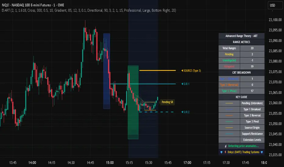
Advanced Range Theory - ART📊 Advanced Range Theory (ART): The Institutional Blueprint
Stop drawing lines. Start reading the blueprint of the market. Advanced Range Theory (ART) is not another support and resistance indicator; it is a military-grade market structure engine designed to decode the language of institutional capital. It operates on a single, powerful premise: markets move in phases of consolidation and expansion, and the key to anticipation lies in understanding the complete lifecycle of these phases.
ART provides a living, breathing map of the battlefield, identifying institutional accumulation zones and tracking them with unparalleled precision from their inception as "Pending" ranges to their ultimate classification after a breakout. This is your X-ray into the market's skeletal structure.
🔬 THEORETICAL FRAMEWORK: THE ARCHITECTURE OF PRICE ACTION
ART is built on a multi-layered system of logic that moves beyond static levels. It treats ranges as dynamic entities with a narrative—a beginning, a middle, and an end. The core of the system is the dynamic classification engine, which analyzes not just the range, but the character of the price action that resolves it.
1. The Range Lifecycle: From Accumulation to Classification
This is the revolutionary heart of ART. A range's true identity is only revealed by how it is broken.
Phase 1: PENDING (Yellow): A new range is identified based on a period of price consolidation (a "parent" candle followed by a minimum number of "inside" candles). At this stage, it is a neutral zone of potential energy—an area where institutions are likely building positions. It is a question the market has not yet answered.
Phase 2: MITIGATION & CLASSIFICATION: When price breaks out and reaches a calculated extension level, the range is considered "mitigated." At this exact moment, ART analyzes the breakout's DNA to classify the range's true intent:
TYPE 1 - BREAKOUT (Blue): Characterized by a strong, impulsive move with confirming volume. This is a high-conviction breakout, signaling aggressive institutional participation and the likely start of a new trend. It is a statement of intent.
TYPE 2 - REVERSAL (Orange): Occurs when price attempts to break one way but is aggressively rejected, reversing and breaking out the other side. This signals absorption and a "failed auction," often marking significant market turning points.
TYPE 3 - PIVOT (Green): A more balanced breakout, lacking the explosive momentum of a Type 1. This often represents a resolution after a period of indecision or a pivot within a larger trading range.
2. The Hierarchical Map: Source & S/R Levels
ART doesn't just draw boxes; it builds a genealogical map of market structure.
SOURCE LEVEL (Thick Gold Line): This is the "genesis" point—the most recently mitigated range. It acts as the primary point of origin for the current market swing and serves as a critical level for determining overall bias. Price action above the Source is generally bullish; below is bearish.
S/R LEVELS (Cyan Lines): When a range is mitigated, the price level where it broke becomes a key Support/Resistance zone for the future. ART tracks the two most recent S/R levels, as these often act as powerful magnets or rejection points for price.
3. The Multi-Factor Validation Engine
To eliminate noise and focus only on institutionally significant ranges, every potential range must pass a rigorous quality control check:
Time-Based Consolidation: Requires a minimum number of consecutive inside candles (minInsideCandles), ensuring a true period of balance.
Volatility-Based Significance: The range's size must be greater than a multiple of the Average True Range (minRangeSize), filtering out insignificant micro-consolidations.
Participation Confirmation: The parent candle of the range is checked against average volume to ensure there was meaningful activity during its formation.
⚙️ THE COMMAND CONSOLE: CONFIGURING YOUR ART ENGINE
Every input is designed to give you granular control over the detection engine, allowing you to tune ART to any market or timeframe with precision. Each tooltip in the script provides a deep dive, but here is a summary of the core controls.
🎯 ART Detection Engine
Minimum Inside Candles: The soul of the detection algorithm. It defines the minimum number of bars that must be contained within a single "parent" candle to qualify as a range. Higher values (3-4) find major, significant consolidation zones. Lower values (1-2) are more sensitive and will identify shorter-term accumulation patterns.
Extension Multiplier & Fibonacci Extension: These control the profit target projections. The Extension Multiplier uses a simple measured move (e.g., 1.0 = a 1:1 projection of the range's height). The Fibonacci Extension uses the golden ratio (1.618) for harmonically-derived targets.
Mitigation Method (Cross vs. Close): Determines how a breakout is confirmed. Cross is more responsive, triggering as soon as price touches the extension. Close is more conservative, requiring a full candle to close beyond the level, which helps filter out fake-outs from wicks.
Min Range Size (ATR): A crucial noise filter. It ensures that ART ignores tiny, insignificant ranges by requiring a range's height to be a certain multiple of the current market volatility (ATR).
📊 Display & Visual Configuration
These settings give you full control over the visual interface. You can toggle every single element—from the Webb Scanner to the S/R Levels—to create a clean or a comprehensive view. Choose a color theme that suits your charting environment or define a fully custom palette.
🕸️ Webb Analysis Scanner
This is a unique real-time flow analysis tool. It draws dynamic, animated lines from the current price to recent historical points. This visualization helps reveal hidden "tendrils" of momentum and short-term support/resistance that are not immediately obvious, acting as a "sonar" for immediate price flow.
📊 THE ANALYTICS HUB: YOUR DASHBOARD DECODED
The dashboard provides a real-time, at-a-glance intelligence briefing on the current state of market structure as seen by the ART engine.
RANGE METRICS: This section is a "census" of the market's structure. It tells you the total number of ranges identified, how many are still Pending (awaiting a breakout), how many are Unmitigated (active but not yet broken), and how many have been Mitigated (classified and complete).
TYPE BREAKDOWN: This is a powerful gauge of market character. A high count of Type 1 (Breakout) ranges suggests a strong, trending environment. A rising number of Type 2 (Reversal) ranges can signal market exhaustion and potential trend changes. A dominant Type 3 (Pivot) count indicates a balanced, rotational market.
KEY GUIDE: The Large dashboard includes a full legend, so you never have to guess what a line or color represents. It's your built-in user manual.
🎨 DECODING THE BLUEPRINT: A VISUAL INTERPRETATION GUIDE
Every line and color in ART is designed for instant, intuitive understanding.
The Range Lines:
Yellow Lines: A Pending range. This is an active zone of accumulation. Pay close attention.
Colored Lines (Blue/Orange/Green): An unmitigated, classified range. The color tells you its breakout character.
Dotted Lines: A Mitigated range. Its story has been told. These historical levels can still act as support or resistance.
The Identification Zones: These colored boxes appear at a range's origin point after it has been classified. They are the "birth certificate" of the range, permanently marking its type (Breakout, Reversal, or Pivot) and providing an immediate visual history of market behavior.
The Hierarchical Lines:
Thick Gold Line (Source): The most important line on your chart. It is the anchor for your bias.
Cyan Lines (S/R): High-probability decision points. Expect reactions here.
Purple Dotted Lines (Extensions): Logical, calculated profit targets for breaking ranges.
🔧 THE ARCHITECT'S VISION: THE DEVELOPMENT JOURNEY
ART was born from a deep frustration with the static and subjective nature of traditional market structure analysis. Drawing lines by hand is inconsistent, and most indicators are reactive, only confirming what has already happened. The goal was to create a proactive, objective, and dynamic framework that could think about the market in terms of phases and lifecycles.
The breakthrough came from a simple shift in perspective: a range's true character isn't defined when it forms, but by how it resolves. This led to the development of the "post-breakout classification engine," which waits for the market to show its hand before assigning a definitive type. The Webb Scanner was inspired by the desire to visualize the unseen, to create a tool that could feel the immediate "pull" and "push" of price flow. The result is not just an indicator; it is a new language for interpreting price action, built on a foundation of logic, clarity, and precision.
⚠️ RISK DISCLAIMER & BEST PRACTICES
Advanced Range Theory is a professional-grade analytical tool designed to enhance a trader's decision-making process. It does not provide direct buy or sell signals. The levels and classifications it generates are based on historical price action and mathematical probabilities. All trading involves substantial risk, and past performance is not indicative of future results. Always use this tool in conjunction with a robust risk management plan.
"I fear not the man who has practiced 10,000 kicks once, but I fear the man who has practiced one kick 10,000 times."
— Dskyz, Trade with insight. Trade with anticipation.
— Bruce Lee
ONE RING 8 MA Bands with RaysCycle analysis tool ...
MAs: Eight moving averages (MA1–MA8) with customizable lengths, types (RMA, WMA, EMA, SMA), and offsets
Bands: Upper/lower bands for each MA, calculated based on final_pctX (Percentage mode) or final_ptsX (Points mode), scaled by multiplier
Rays: Forward-projected lines for bands, with customizable start points, styles (Solid, Dashed, Dotted), and lengths (up to 500 bars)
Band Choices
Manual: Uses individual inputs for band offsets
Uniform: Sets all offsets to base_pct (e.g., 0.1%) or base_pts (e.g., 0.1 points)
Linear: Scales linearly (e.g., base_pct * 1, base_pct * 2, base_pct * 3 ..., base_pct * 8)
Exponential: Scales exponentially (e.g., base_pct * 1, base_pct * 2, base_pct * 4, base_pct * 8 ..., base_pct * 128)
ATR-Based: Offsets are derived from the Average True Range (ATR), scaled by a linear factor. Dynamic bands that adapt to market conditions, useful for breakout or mean-reversion strategies. (final_pct1 = base_pct * atr, final_pct2 = base_pct * atr * 2, ..., final_pct8 = base_pct * atr * 8)
Geometric: Offsets follow a geometric progression (e.g., base_pct * r^0, base_pct * r^1, base_pct * r^2, ..., where r is a ratio like 1.5) This is less aggressive than Exponential (which uses powers of 2) and provides a smoother progression.
Example: If base_pct = 0.1, r = 1.5, then final_pct1 = 0.1%, final_pct2 = 0.15%, final_pct3 = 0.225%, ..., final_pct8 ≈ 1.71%
Harmonic: Offsets are based on harmonic flavored ratios. final_pctX = base_pct * X / (9 - X), final_ptsX = base_pts * X / (9 - X) for X = 1 to 8 This creates a harmonic-like progression where offsets increase non-linearly, ensuring MA8 bands are wider than MA1 bands, and avoids duplicating the Linear choice above.
Ex. offsets for base_pct = 0.1: MA1: ±0.0125% (0.1 * 1/8), MA2: ±0.0286% (0.1 * 2/7), MA3: ±0.05% (0.1 * 3/6), MA4: ±0.08% (0.1 * 4/5), MA5: ±0.125% (0.1 * 5/4), MA6: ±0.2% (0.1 * 6/3), MA7: ±0.35% (0.1 * 7/2), MA8: ±0.8% (0.1 * 8/1)
Square Root: Offsets grow with the square root of the band index (e.g., base_pct * sqrt(1), base_pct * sqrt(2), ..., base_pct * sqrt(8)). This creates a gradual widening, less aggressive than Linear or Exponential. Set final_pct1 = base_pct * sqrt(1), final_pct2 = base_pct * sqrt(2), ..., final_pct8 = base_pct * sqrt(8).
Example: If base_pct = 0.1, then final_pct1 = 0.1%, final_pct2 ≈ 0.141%, final_pct3 ≈ 0.173%, ..., final_pct8 ≈ 0.283%.
Fibonacci: Uses Fibonacci ratios (e.g., base_pct * 1, base_pct * 1.618, base_pct * 2.618
Percentage vs. Points Toggle:
In Percentage mode, bands are calculated as ma * (1 ± (final_pct / 100) * multiplier)
In Points mode, bands are calculated as ma ± final_pts * multiplier, where final_pts is in price units.
Threshold Setting for Slope:
Threshold setting for determining when the slope would be significant enough to call it a change in direction. Can check efficiency by setting MA1 to color on slope temporarily
Arrow table: Shows slope direction of 8 MAs using an Up or Down triangle, or shows Flat condition if no triangle.

BAERMThe Bitcoin Auto-correlation Exchange Rate Model: A Novel Two Step Approach
THIS IS NOT FINANCIAL ADVICE. THIS ARTICLE IS FOR EDUCATIONAL AND ENTERTAINMENT PURPOSES ONLY.
If you enjoy this software and information, please consider contributing to my lightning address
Prelude
It has been previously established that the Bitcoin daily USD exchange rate series is extremely auto-correlated
In this article, we will utilise this fact to build a model for Bitcoin/USD exchange rate. But not a model for predicting the exchange rate, but rather a model to understand the fundamental reasons for the Bitcoin to have this exchange rate to begin with.
This is a model of sound money, scarcity and subjective value.
Introduction
Bitcoin, a decentralised peer to peer digital value exchange network, has experienced significant exchange rate fluctuations since its inception in 2009. In this article, we explore a two-step model that reasonably accurately captures both the fundamental drivers of Bitcoin’s value and the cyclical patterns of bull and bear markets. This model, whilst it can produce forecasts, is meant more of a way of understanding past exchange rate changes and understanding the fundamental values driving the ever increasing exchange rate. The forecasts from the model are to be considered inconclusive and speculative only.
Data preparation
To develop the BAERM, we used historical Bitcoin data from Coin Metrics, a leading provider of Bitcoin market data. The dataset includes daily USD exchange rates, block counts, and other relevant information. We pre-processed the data by performing the following steps:
Fixing date formats and setting the dataset’s time index
Generating cumulative sums for blocks and halving periods
Calculating daily rewards and total supply
Computing the log-transformed price
Step 1: Building the Base Model
To build the base model, we analysed data from the first two epochs (time periods between Bitcoin mining reward halvings) and regressed the logarithm of Bitcoin’s exchange rate on the mining reward and epoch. This base model captures the fundamental relationship between Bitcoin’s exchange rate, mining reward, and halving epoch.
where Yt represents the exchange rate at day t, Epochk is the kth epoch (for that t), and epsilont is the error term. The coefficients beta0, beta1, and beta2 are estimated using ordinary least squares regression.
Base Model Regression
We use ordinary least squares regression to estimate the coefficients for the betas in figure 2. In order to reduce the possibility of over-fitting and ensure there is sufficient out of sample for testing accuracy, the base model is only trained on the first two epochs. You will notice in the code we calculate the beta2 variable prior and call it “phaseplus”.
The code below shows the regression for the base model coefficients:
\# Run the regression
mask = df\ < 2 # we only want to use Epoch's 0 and 1 to estimate the coefficients for the base model
reg\_X = df.loc\ [mask, \ \].shift(1).iloc\
reg\_y = df.loc\ .iloc\
reg\_X = sm.add\_constant(reg\_X)
ols = sm.OLS(reg\_y, reg\_X).fit()
coefs = ols.params.values
print(coefs)
The result of this regression gives us the coefficients for the betas of the base model:
\
or in more human readable form: 0.029, 0.996869586, -0.00043. NB that for the auto-correlation/momentum beta, we did NOT round the significant figures at all. Since the momentum is so important in this model, we must use all available significant figures.
Fundamental Insights from the Base Model
Momentum effect: The term 0.997 Y suggests that the exchange rate of Bitcoin on a given day (Yi) is heavily influenced by the exchange rate on the previous day. This indicates a momentum effect, where the price of Bitcoin tends to follow its recent trend.
Momentum effect is a phenomenon observed in various financial markets, including stocks and other commodities. It implies that an asset’s price is more likely to continue moving in its current direction, either upwards or downwards, over the short term.
The momentum effect can be driven by several factors:
Behavioural biases: Investors may exhibit herding behaviour or be subject to cognitive biases such as confirmation bias, which could lead them to buy or sell assets based on recent trends, reinforcing the momentum.
Positive feedback loops: As more investors notice a trend and act on it, the trend may gain even more traction, leading to a self-reinforcing positive feedback loop. This can cause prices to continue moving in the same direction, further amplifying the momentum effect.
Technical analysis: Many traders use technical analysis to make investment decisions, which often involves studying historical exchange rate trends and chart patterns to predict future exchange rate movements. When a large number of traders follow similar strategies, their collective actions can create and reinforce exchange rate momentum.
Impact of halving events: In the Bitcoin network, new bitcoins are created as a reward to miners for validating transactions and adding new blocks to the blockchain. This reward is called the block reward, and it is halved approximately every four years, or every 210,000 blocks. This event is known as a halving.
The primary purpose of halving events is to control the supply of new bitcoins entering the market, ultimately leading to a capped supply of 21 million bitcoins. As the block reward decreases, the rate at which new bitcoins are created slows down, and this can have significant implications for the price of Bitcoin.
The term -0.0004*(50/(2^epochk) — (epochk+1)²) accounts for the impact of the halving events on the Bitcoin exchange rate. The model seems to suggest that the exchange rate of Bitcoin is influenced by a function of the number of halving events that have occurred.
Exponential decay and the decreasing impact of the halvings: The first part of this term, 50/(2^epochk), indicates that the impact of each subsequent halving event decays exponentially, implying that the influence of halving events on the Bitcoin exchange rate diminishes over time. This might be due to the decreasing marginal effect of each halving event on the overall Bitcoin supply as the block reward gets smaller and smaller.
This is antithetical to the wrong and popular stock to flow model, which suggests the opposite. Given the accuracy of the BAERM, this is yet another reason to question the S2F model, from a fundamental perspective.
The second part of the term, (epochk+1)², introduces a non-linear relationship between the halving events and the exchange rate. This non-linear aspect could reflect that the impact of halving events is not constant over time and may be influenced by various factors such as market dynamics, speculation, and changing market conditions.
The combination of these two terms is expressed by the graph of the model line (see figure 3), where it can be seen the step from each halving is decaying, and the step up from each halving event is given by a parabolic curve.
NB - The base model has been trained on the first two halving epochs and then seeded (i.e. the first lag point) with the oldest data available.
Constant term: The constant term 0.03 in the equation represents an inherent baseline level of growth in the Bitcoin exchange rate.
In any linear or linear-like model, the constant term, also known as the intercept or bias, represents the value of the dependent variable (in this case, the log-scaled Bitcoin USD exchange rate) when all the independent variables are set to zero.
The constant term indicates that even without considering the effects of the previous day’s exchange rate or halving events, there is a baseline growth in the exchange rate of Bitcoin. This baseline growth could be due to factors such as the network’s overall growth or increasing adoption, or changes in the market structure (more exchanges, changes to the regulatory environment, improved liquidity, more fiat on-ramps etc).
Base Model Regression Diagnostics
Below is a summary of the model generated by the OLS function
OLS Regression Results
\==============================================================================
Dep. Variable: logprice R-squared: 0.999
Model: OLS Adj. R-squared: 0.999
Method: Least Squares F-statistic: 2.041e+06
Date: Fri, 28 Apr 2023 Prob (F-statistic): 0.00
Time: 11:06:58 Log-Likelihood: 3001.6
No. Observations: 2182 AIC: -5997.
Df Residuals: 2179 BIC: -5980.
Df Model: 2
Covariance Type: nonrobust
\==============================================================================
coef std err t P>|t| \
\------------------------------------------------------------------------------
const 0.0292 0.009 3.081 0.002 0.011 0.048
logprice 0.9969 0.001 1012.724 0.000 0.995 0.999
phaseplus -0.0004 0.000 -2.239 0.025 -0.001 -5.3e-05
\==============================================================================
Omnibus: 674.771 Durbin-Watson: 1.901
Prob(Omnibus): 0.000 Jarque-Bera (JB): 24937.353
Skew: -0.765 Prob(JB): 0.00
Kurtosis: 19.491 Cond. No. 255.
\==============================================================================
Below we see some regression diagnostics along with the regression itself.
Diagnostics: We can see that the residuals are looking a little skewed and there is some heteroskedasticity within the residuals. The coefficient of determination, or r2 is very high, but that is to be expected given the momentum term. A better r2 is manually calculated by the sum square of the difference of the model to the untrained data. This can be achieved by the following code:
\# Calculate the out-of-sample R-squared
oos\_mask = df\ >= 2
oos\_actual = df.loc\
oos\_predicted = df.loc\
residuals\_oos = oos\_actual - oos\_predicted
SSR = np.sum(residuals\_oos \*\* 2)
SST = np.sum((oos\_actual - oos\_actual.mean()) \*\* 2)
R2\_oos = 1 - SSR/SST
print("Out-of-sample R-squared:", R2\_oos)
The result is: 0.84, which indicates a very close fit to the out of sample data for the base model, which goes some way to proving our fundamental assumption around subjective value and sound money to be accurate.
Step 2: Adding the Damping Function
Next, we incorporated a damping function to capture the cyclical nature of bull and bear markets. The optimal parameters for the damping function were determined by regressing on the residuals from the base model. The damping function enhances the model’s ability to identify and predict bull and bear cycles in the Bitcoin market. The addition of the damping function to the base model is expressed as the full model equation.
This brings me to the question — why? Why add the damping function to the base model, which is arguably already performing extremely well out of sample and providing valuable insights into the exchange rate movements of Bitcoin.
Fundamental reasoning behind the addition of a damping function:
Subjective Theory of Value: The cyclical component of the damping function, represented by the cosine function, can be thought of as capturing the periodic fluctuations in market sentiment. These fluctuations may arise from various factors, such as changes in investor risk appetite, macroeconomic conditions, or technological advancements. Mathematically, the cyclical component represents the frequency of these fluctuations, while the phase shift (α and β) allows for adjustments in the alignment of these cycles with historical data. This flexibility enables the damping function to account for the heterogeneity in market participants’ preferences and expectations, which is a key aspect of the subjective theory of value.
Time Preference and Market Cycles: The exponential decay component of the damping function, represented by the term e^(-0.0004t), can be linked to the concept of time preference and its impact on market dynamics. In financial markets, the discounting of future cash flows is a common practice, reflecting the time value of money and the inherent uncertainty of future events. The exponential decay in the damping function serves a similar purpose, diminishing the influence of past market cycles as time progresses. This decay term introduces a time-dependent weight to the cyclical component, capturing the dynamic nature of the Bitcoin market and the changing relevance of past events.
Interactions between Cyclical and Exponential Decay Components: The interplay between the cyclical and exponential decay components in the damping function captures the complex dynamics of the Bitcoin market. The damping function effectively models the attenuation of past cycles while also accounting for their periodic nature. This allows the model to adapt to changing market conditions and to provide accurate predictions even in the face of significant volatility or structural shifts.
Now we have the fundamental reasoning for the addition of the function, we can explore the actual implementation and look to other analogies for guidance —
Financial and physical analogies to the damping function:
Mathematical Aspects: The exponential decay component, e^(-0.0004t), attenuates the amplitude of the cyclical component over time. This attenuation factor is crucial in modelling the diminishing influence of past market cycles. The cyclical component, represented by the cosine function, accounts for the periodic nature of market cycles, with α determining the frequency of these cycles and β representing the phase shift. The constant term (+3) ensures that the function remains positive, which is important for practical applications, as the damping function is added to the rest of the model to obtain the final predictions.
Analogies to Existing Damping Functions: The damping function in the BAERM is similar to damped harmonic oscillators found in physics. In a damped harmonic oscillator, an object in motion experiences a restoring force proportional to its displacement from equilibrium and a damping force proportional to its velocity. The equation of motion for a damped harmonic oscillator is:
x’’(t) + 2γx’(t) + ω₀²x(t) = 0
where x(t) is the displacement, ω₀ is the natural frequency, and γ is the damping coefficient. The damping function in the BAERM shares similarities with the solution to this equation, which is typically a product of an exponential decay term and a sinusoidal term. The exponential decay term in the BAERM captures the attenuation of past market cycles, while the cosine term represents the periodic nature of these cycles.
Comparisons with Financial Models: In finance, damped oscillatory models have been applied to model interest rates, stock prices, and exchange rates. The famous Black-Scholes option pricing model, for instance, assumes that stock prices follow a geometric Brownian motion, which can exhibit oscillatory behavior under certain conditions. In fixed income markets, the Cox-Ingersoll-Ross (CIR) model for interest rates also incorporates mean reversion and stochastic volatility, leading to damped oscillatory dynamics.
By drawing on these analogies, we can better understand the technical aspects of the damping function in the BAERM and appreciate its effectiveness in modelling the complex dynamics of the Bitcoin market. The damping function captures both the periodic nature of market cycles and the attenuation of past events’ influence.
Conclusion
In this article, we explored the Bitcoin Auto-correlation Exchange Rate Model (BAERM), a novel 2-step linear regression model for understanding the Bitcoin USD exchange rate. We discussed the model’s components, their interpretations, and the fundamental insights they provide about Bitcoin exchange rate dynamics.
The BAERM’s ability to capture the fundamental properties of Bitcoin is particularly interesting. The framework underlying the model emphasises the importance of individuals’ subjective valuations and preferences in determining prices. The momentum term, which accounts for auto-correlation, is a testament to this idea, as it shows that historical price trends influence market participants’ expectations and valuations. This observation is consistent with the notion that the price of Bitcoin is determined by individuals’ preferences based on past information.
Furthermore, the BAERM incorporates the impact of Bitcoin’s supply dynamics on its price through the halving epoch terms. By acknowledging the significance of supply-side factors, the model reflects the principles of sound money. A limited supply of money, such as that of Bitcoin, maintains its value and purchasing power over time. The halving events, which reduce the block reward, play a crucial role in making Bitcoin increasingly scarce, thus reinforcing its attractiveness as a store of value and a medium of exchange.
The constant term in the model serves as the baseline for the model’s predictions and can be interpreted as an inherent value attributed to Bitcoin. This value emphasizes the significance of the underlying technology, network effects, and Bitcoin’s role as a medium of exchange, store of value, and unit of account. These aspects are all essential for a sound form of money, and the model’s ability to account for them further showcases its strength in capturing the fundamental properties of Bitcoin.
The BAERM offers a potential robust and well-founded methodology for understanding the Bitcoin USD exchange rate, taking into account the key factors that drive it from both supply and demand perspectives.
In conclusion, the Bitcoin Auto-correlation Exchange Rate Model provides a comprehensive fundamentally grounded and hopefully useful framework for understanding the Bitcoin USD exchange rate.

Draw Line For High Low Custom Range Interactive█ OVERVIEW
This indicator is an educational indicator to make pine coders easier to how to use interactive inputs with User-Defined Type (UDT) especially when dealing input.time.
█ NOTES
This indicator is not perfect but it is a good starting point or template to start develop custom range interactive indicator.
█ INSPIRATIONS
ABC 123 Harmonic Ratio Custom Range Interactive
XABCD Harmonic Pattern Custom Range Interactive
PriceTimeInteractive
█ CREDITS
CAGR Custom Range
Pine scripts are now interactive
█ FEATURES
1. High Low points are determined based on points selected.
2. Line will be drawn after points are correctly arranged.
3. Label show error once wrong point is selected, move the point as instructed in example.
█ EXAMPLES / USAGE

eHarmonicpatternsLogScaleLibrary "eHarmonicpatternsLogScale"
Library provides functions to scan harmonic patterns both or normal and log scale
getSupportedPatterns()
get_prz_range(x, a, b, c, patternArray, errorPercent, start_adj, end_adj, logScale)
Provides PRZ range based on BCD and XAD ranges
Parameters:
x : X coordinate value
a : A coordinate value
b : B coordinate value
c : C coordinate value
patternArray : Pattern flags for which PRZ range needs to be calculated
errorPercent : Error threshold
start_adj : - Adjustments for entry levels
end_adj : - Adjustments for stop levels
logScale : - calculate on log scale. Default is false
Returns: Start and end of consolidated PRZ range
get_prz_range_xad(x, a, b, c, patternArray, errorPercent, start_adj, end_adj, logScale)
Provides PRZ range based on XAD range only
Parameters:
x : X coordinate value
a : A coordinate value
b : B coordinate value
c : C coordinate value
patternArray : Pattern flags for which PRZ range needs to be calculated
errorPercent : Error threshold
start_adj : - Adjustments for entry levels
end_adj : - Adjustments for stop levels
logScale : - calculate on log scale. Default is false
Returns: Start and end of consolidated PRZ range
get_projection_range(x, a, b, c, patternArray, errorPercent, start_adj, end_adj, logScale)
Provides Projection range based on BCD and XAD ranges
Parameters:
x : X coordinate value
a : A coordinate value
b : B coordinate value
c : C coordinate value
patternArray : Pattern flags for which PRZ range needs to be calculated
errorPercent : Error threshold
start_adj : - Adjustments for entry levels
end_adj : - Adjustments for stop levels
logScale : - calculate on log scale. Default is false
Returns: Array containing start and end ranges
isHarmonicPattern(x, a, b, c, d, flags, defaultEnabled, errorPercent, logScale)
Checks for harmonic patterns
Parameters:
x : X coordinate value
a : A coordinate value
b : B coordinate value
c : C coordinate value
d : D coordinate value
flags : flags to check patterns. Send empty array to enable all
defaultEnabled
errorPercent : Error threshold
logScale : - calculate on log scale. Default is false
Returns: Array of boolean values which says whether valid pattern exist and array of corresponding pattern names
isHarmonicProjection(x, a, b, c, flags, defaultEnabled, errorPercent, logScale)
Checks for harmonic pattern projection
Parameters:
x : X coordinate value
a : A coordinate value
b : B coordinate value
c : C coordinate value
flags : flags to check patterns. Send empty array to enable all
defaultEnabled
errorPercent : Error threshold
logScale : - calculate on log scale. Default is false
Returns: Array of boolean values which says whether valid pattern exist and array of corresponding pattern names.

God Number Channel v2(GNC v2)GNC got a little update:
1) Logic changed a bit.
I tried to calculate MAs based on the power(high - low of previous bars).You can see it the M-variables, as new statements were added in calculation section of MAs. I don't really know if I did right, because I didn't go too much in Pine Script. I just wanted to make a Bollinger-bands-like bands, which could predict the levels at which might reverse, using legendary fibonacci and Tesla's harmonic number 432. It's might sound as a joke, but as you can see, it works pretty good.
2) Customization :
No need to change Fibonacci ratios in code. Now you can do it in the GNC settings. Also MAs' names were made obvious, just check it out. Time of million similar "MA n1" has passed :)
3) Trade-entry advices :
I didn't tell you exactly the trade-entry advices, as I haven't explored this script fully yet :) But you probably understood something intuitively, when added GNC on the chart. Now I made things way more obvious:
1. Zones between Fib ratios show you how aware you should be of price movements. Basically, here are the rules, but you probably understand them already:
1.1 Red zone(RZ) : high awareness, very likly for price to be reversed, but if there is a clear trend and you know, than it might be a time for price to shoot up/down.
1.2 Orange zone(OZ) : medium awareness, not so obvious, as price might go between boundaries of OZ and continue the trend movement if such followed before entering the OZ. If price go below lower boundary of OZ and the next bar opens below this boundary, it might be a signal for SHORY, BUT(!) please consider confirmation of any sort to be more sure. Think of going beyond the upper boundary by analogy.
1.3 Green Zone(GZ) : if the price hits any boundary of green zone, it is usually a good oppurtunity to open a position against the movement(hit lower boundary -> open LONG, hit upper boundary -> open SHORT).
1.4 Middle Zone(Harmonic Zone)(MZ) : same rules from Green Zone.
IMPORTANT RECCOMENDATION : Use trend indicator to trend all signals from zones to follow the trend, 'cause counter-trending with this thing without stop loss might very quickly wipe you out , might if you will counter-trend strategy with GNC, I will be glad if you share it with the community :)
Reccomendation for better entries :
1) if the price hits the lower(or high) boundaries(LB or HB) zone after zone(hit LB or HB of RZ, then of OZ, then of GZ), it is a very good signal to either LONG, if price was hitting LBs , or SHORT, if hitting HBs .
2) Consider NOT to place trades when in MZ, as price in this zone gets tricky often enough. By the way, if you dont the see the harmonic MAs(which go with plot(ma1+(0.432*avg1)) ), then set the transparency of zone to 20% or a bit more and then it will be ok.
I will continue to develop the GNC and any help or feedback from you, guys, will be very helpful for me, so you welcome for any of those, but please be precise in your critics.
Thank you for using my stuff, hope you found it usefull. Good luck :)

.b pin-up symbolWhen trading cryptocoins, it is necessary to check the price trend of NASDAQ, BTC.D, BTC.OI, BTC spot or other coins of similar groups.
However it is very cumbersome to put a comparison symbol in the Tradingview chart and combine individual indicators one by one.
Moreover even with such a combination, the chart is messy and visibility is not good.
This script was developed as a composite-solution to that situation, and will make you happy.
- NQ1!, USTECH100CFD | symbol fixed
- BTC.Dominance, BTC.OpenInterest, BTC symbol, others pin-up-symbol | selectable
- Pin-up-symbol | selectable
- Pin-up-symbol's candle chart
- Trending
* EMA 9,21,50,200 ribbon classic EMA
* .b price line ; .b price = unique trending price with price-action + relative-volume-action + ATR
* Dynamic S/R Cloud ; BB + donchian band + high/low + atr mixed custom-logic
* VWWMA + .b price Shadow ; Volume-weighted WMA on .b price = unique MA faster than classic VWMA
Trending shadow direction is not bad even on low-timeframe (1, 2, 3, 5m, 15m...)
- Pattern
* Harmonic Pattern ; A simplified version of the harmonic pattern indicator, simply show-up pattern complete position
for reference only - adopted from HeWhoMustNotBeNamed's script.
- Information Panel
* BTC Dominance, BTC Open Interest, Pin-Up-Symbol price
* Trend meter ; 5,15,30,1h,2h,4h Meter Calc with 1 minute-timeframe candles
5 = Green if the current price is higher than the price 5 minutes ago.
1h = Green if the current price is higher than the price 2 hours ago.
4h = Red if the current price is lower than the price 4 hours ago.
* caution ; To use real-time chart of "CME_MINI:NQ1!" you have to additional subscribe CME data,
default setting is 'NQ1!' , you can change to 'USTECH100CFD'
* When you choose symbol which is closed trading hours, the script's update stopped.
Even if the selected pin-up-symbol is on trading hours, the currently selected symbol's chart doesn't update.
* recommended | chart setting > Appearance : Top margin 0%, Bottom margin 0% for optimized screen usage :)
if you have any questions freely contact to me by message on tradingview, or telegram @sr_bt
but please understand that responses may be quite late.
------------------------------------------------------------------------------------------------------------------------------------------------------------
copyright 2022 (sr_b)
Special thanks to all of contributors of community.
The script (originaly .b) may be freely distributed under the MIT license.
The other classic script code also may be freely distributed under the MIT license.
Simplified Harmonic script part | core adopted from 'Multi ZigZag Harmonic Patterns (HeWhoMustNotBeNamed)' MPL2.0 license
statisticsLibrary "statistics"
General statistics library.
erf(x) The "error function" encountered in integrating the normal
distribution (which is a normalized form of the Gaussian function).
Parameters:
x : The input series.
Returns: The Error Function evaluated for each element of x.
erfc(x)
Parameters:
x : The input series
Returns: The Complementary Error Function evaluated for each alement of x.
sumOfReciprocals(src, len) Calculates the sum of the reciprocals of the series.
For each element 'elem' in the series:
sum += 1/elem
Should the element be 0, the reciprocal value of 0 is used instead
of NA.
Parameters:
src : The input series.
len : The length for the sum.
Returns: The sum of the resciprocals of 'src' for 'len' bars back.
mean(src, len) The mean of the series.
(wrapper around ta.sma).
Parameters:
src : The input series.
len : The length for the mean.
Returns: The mean of 'src' for 'len' bars back.
average(src, len) The mean of the series.
(wrapper around ta.sma).
Parameters:
src : The input series.
len : The length for the average.
Returns: The average of 'src' for 'len' bars back.
geometricMean(src, len) The Geometric Mean of the series.
The geometric mean is most important when using data representing
percentages, ratios, or rates of change. It cannot be used for
negative numbers
Since the pure mathematical implementation generates a very large
intermediate result, we performed the calculation in log space.
Parameters:
src : The input series.
len : The length for the geometricMean.
Returns: The geometric mean of 'src' for 'len' bars back.
harmonicMean(src, len) The Harmonic Mean of the series.
The harmonic mean is most applicable to time changes and, along
with the geometric mean, has been used in economics for price
analysis. It is more difficult to calculate; therefore, it is less
popular than eiter of the other averages.
0 values are ignored in the calculation.
Parameters:
src : The input series.
len : The length for the harmonicMean.
Returns: The harmonic mean of 'src' for 'len' bars back.
median(src, len) The median of the series.
(a wrapper around ta.median)
Parameters:
src : The input series.
len : The length for the median.
Returns: The median of 'src' for 'len' bars back.
variance(src, len, biased) The variance of the series.
Parameters:
src : The input series.
len : The length for the variance.
biased : Wether to use the biased calculation (for a population), or the
unbiased calculation (for a sample set). .
Returns: The variance of 'src' for 'len' bars back.
stdev(src, len, biased) The standard deviation of the series.
Parameters:
src : The input series.
len : The length for the stdev.
biased : Wether to use the biased calculation (for a population), or the
unbiased calculation (for a sample set). .
Returns: The standard deviation of 'src' for 'len' bars back.
skewness(src, len) The skew of the series.
Skewness measures the amount of distortion from a symmetric
distribution, making the curve appear to be short on the left
(lower prices) and extended to the right (higher prices). The
extended side, either left or right is called the tail, and a
longer tail to the right is called positive skewness. Negative
skewness has the tail extending towards the left.
Parameters:
src : The input series.
len : The length for the skewness.
Returns: The skewness of 'src' for 'len' bars back.
kurtosis(src, len) The kurtosis of the series.
Kurtosis describes the peakedness or flatness of a distribution.
This can be used as an unbiased assessment of whether prices are
trending or moving sideways. Trending prices will ocver a wider
range and thus a flatter distribution (kurtosis < 3; negative
kurtosis). If prices are range-bound, there will be a clustering
around the mean and we have positive kurtosis (kurtosis > 3)
Parameters:
src : The input series.
len : The length for the kurtosis.
Returns: The kurtosis of 'src' for 'len' bars back.
excessKurtosis(src, len) The normalized kurtosis of the series.
kurtosis > 0 --> positive kurtosis --> trending
kurtosis < 0 --> negative krutosis --> range-bound
Parameters:
src : The input series.
len : The length for the excessKurtosis.
Returns: The excessKurtosis of 'src' for 'len' bars back.
normDist(src, len, value) Calculates the probability mass for the value according to the
src and length. It calculates the probability for value to be
present in the normal distribution calculated for src and length.
Parameters:
src : The input series.
len : The length for the normDist.
value : The series of values to calculate the normal distance for
Returns: The normal distance of 'value' to 'src' for 'len' bars back.
normDistCumulative(src, len, value) Calculates the cumulative probability mass for the value according
to the src and length. It calculates the cumulative probability for
value to be present in the normal distribution calculated for src
and length.
Parameters:
src : The input series.
len : The length for the normDistCumulative.
value : The series of values to calculate the cumulative normal distance
for
Returns: The cumulative normal distance of 'value' to 'src' for 'len' bars
back.
zScore(src, len, value) Returns then z-score of objective to the series src.
It returns the number of stdev's the objective is away from the
mean(src, len)
Parameters:
src : The input series.
len : The length for the zScore.
value : The series of values to calculate the cumulative normal distance
for
Returns: The z-score of objectiv with respect to src and len.
er(src, len) Calculates the efficiency ratio of the series.
It measures the noise of the series. The lower the number, the
higher the noise.
Parameters:
src : The input series.
len : The length for the efficiency ratio.
Returns: The efficiency ratio of 'src' for 'len' bars back.
efficiencyRatio(src, len) Calculates the efficiency ratio of the series.
It measures the noise of the series. The lower the number, the
higher the noise.
Parameters:
src : The input series.
len : The length for the efficiency ratio.
Returns: The efficiency ratio of 'src' for 'len' bars back.
fractalEfficiency(src, len) Calculates the efficiency ratio of the series.
It measures the noise of the series. The lower the number, the
higher the noise.
Parameters:
src : The input series.
len : The length for the efficiency ratio.
Returns: The efficiency ratio of 'src' for 'len' bars back.
mse(src, len) Calculates the Mean Squared Error of the series.
Parameters:
src : The input series.
len : The length for the mean squared error.
Returns: The mean squared error of 'src' for 'len' bars back.
meanSquaredError(src, len) Calculates the Mean Squared Error of the series.
Parameters:
src : The input series.
len : The length for the mean squared error.
Returns: The mean squared error of 'src' for 'len' bars back.
rmse(src, len) Calculates the Root Mean Squared Error of the series.
Parameters:
src : The input series.
len : The length for the root mean squared error.
Returns: The root mean squared error of 'src' for 'len' bars back.
rootMeanSquaredError(src, len) Calculates the Root Mean Squared Error of the series.
Parameters:
src : The input series.
len : The length for the root mean squared error.
Returns: The root mean squared error of 'src' for 'len' bars back.
mae(src, len) Calculates the Mean Absolute Error of the series.
Parameters:
src : The input series.
len : The length for the mean absolute error.
Returns: The mean absolute error of 'src' for 'len' bars back.
meanAbsoluteError(src, len) Calculates the Mean Absolute Error of the series.
Parameters:
src : The input series.
len : The length for the mean absolute error.
Returns: The mean absolute error of 'src' for 'len' bars back.

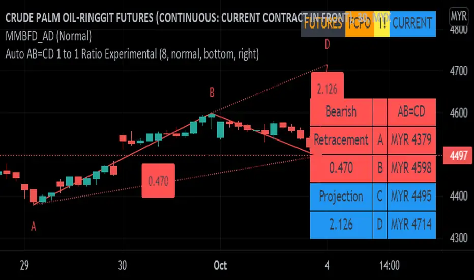
Auto AB=CD 1 to 1 Ratio ExperimentalThis indicator was experimental based AB=CD, shows last AB=CD either Standard AB=CD or Reciprocal AB=CD which uses time instead of bar_index.
This build is based upon educational materials (refer below resources).
ABCD are based on 1 to 1 Ratio for price and time.
Features / Pros:
1. Show last AB=CD points and lines including table value.
2. Customize table position and size.
3. For desktop display only, not for mobile.
Cons:
1. Time for point D less accurate for intraday timeframe (minute, hour, etc) which may including holidays and depends on price volatility.
2. Label ratio not shown properly depends on timeframe especially for intraday timeframe and maybe for Daily and Weekly timeframe.
3. Experimental code, use at your own risk.
FAQ
1. Credits
Scott M Carney, Harmonic Trading: Volume One and Two.
LonesomeTheBlue for zigzag array source code.
HeWhoMustNotBeNamed for some guidance and advice.
2. Previous Build / Resources
Link 1
Link 2
Link 3
Link 4
3. Code Usage
Free to use for personal usage.
Left : Bullish AB=CD, Right : Bullish Reciprocal AB=CD
Left : Bearish AB=CD, Right : Bearish Reciprocal AB=CD
Pythagorean Moving Averages (and more)When you think of the question "take the mean of this dataset", you'd normally think of using the arithmetic mean because usually the norm is equal to 1; however, there are an infinite number of other types of means depending on the function norm (p).
Pythagoras' is credited for the main types of means: his harmonic mean, his geometric mean, and his arithmetic mean:
Harmonic Average (p = -1):
- Take the reciprocal of all the numbers in the dataset, add them all together, divide by the amount of numbers added together, then take the reciprocal of the final answer.
Geometric Average (p = 0):
- Multiply all the numbers in the dataset, then take the nth root where n is equal to the amount of number you multiplied together.
Arithmetic Mean (p = 1):
- Add all the numbers in the dataset, then divide by the amount of numbers you added by.
A couple other means included in this script were the quadratic mean (p = 2) and the cubic mean (p = 3).
Quadratic Mean (p = 2):
- Square every number in the dataset, then divide by the amount of numbers your added by, then take the square root.
Cubic Mean (p = 3):
- Cube every number in the dataset, then divide by the amount of numbers you added by, then take the cube root.
There are an infinite number of means for every scenario of p, but they begin to follow a pattern after p = 3.
Read more:
www.cs.uni.edu
en.wikipedia.org
en.wikipedia.org
Note : I added the functions for the quadratic mean and cubic mean, but since market charts don't have those types of graphs, the functions don't usually work. It's the same reason why sometimes you'll see the harmonic average not working.
Disclaimer : This is not financial or mathematical advice, please look for someone certified before making any decisions.

Detrended Rhythm Oscillator (DRO)How to detect the current "market beat" or market cycle?
A common way to capture the current dominant cycle length is to detrend the price and look for common rhythms in the detrended series. A common approach is to use a Detrended Price Oscillator (DPO). This is done in order to identify and isolate short-term cycles.
A basic DPO description can be found here:
www.tradingview.com
Improvements to the standard DPO
The main purpose of the standard DPO is to analyze historical data in order to observe cycle's in a market's movement. DPO can give the technical analyst a better sense of a cycle's typical high/low range as well as its duration. However, you need to manually try to "see" tops and bottoms on the detrended price and measure manually the distance from low-low or high-high in order to derive a possible cycle length.
Therefore, I added the following improvements:
1) Using a DPO to detrend the price
2) Indicate the turns of the detrended price with a ZigZag lines to better see the tops/bottoms
3) Detrend the ZigZag to remove price amplitude between turns to even better see the cyclic turns ("rhythm")
4) Measure the distance from last detrended zigzag pivot (high-high / low-low) and plot the distance in bars above/below the turn
Now, you can clearly see the rhythm of the dataset indicated by the Detrended Rhythm Oscillator including the exact length between the turns. This makes the procedure to "spot" turns and "measure" distance more simple for the trader.
How to use this information
The purpose is to check if there is a common rhythm or beat in the underlying dataset. To check that, look for recurring pattern in the numbers. E.g. if you often see the same measured distance, you can conclude that there is a major dominant cycle in this market. Also watch for harmonic relations between the numbers. So in the example above you see the highlighted cluster of detected length of around 40,80 and 120. There three numbers all have a harmonic relation to 40.
Once you have this cyclic information, you can use this number to optimize or tune technical indicators based on the current dominant cycle length. E.g. set the length parameter of a technical indicator to the detected harmonic length with the DRO indicator.
Example Use-Case
You can use this information to set the input for the following free public open-source script:
Disclaimer
This is not meant to be a technical indicator on its own and the derived cyclic length should not be used to forecast the next turn per se. The indicator should give you an indication of the current market beat or dominant beats which can be use to further optimize other oscillator or trading related settings.
Options & settings
The indicator allows to plot different versions. It allows to plot the original DPO, the DRO with ZigZag lines, the DRO with detrended ZigZag lines and length labels on/off. You can turn on or off these version in the indicator settings. So you can tweak it visually to your own needs.

EMA20 MA50 MA200 + T3-CCIEMA20 MA50 MA200 + T3-CCI
This combination of triple Moving Average and CCI is a strategy to be used in conjunction with Harmonical Patterns and Fibonacci Rations .
Heikin Ashi price can be used as the price source for the Moving Averages and the T3-CCI, instead of the real price.
Two instances of the indicator can be spawned to have both the triple MAs and the T3-CCI on the chart (L-Click on the Indicator > Move To > New Pane Below).
Alerts are available to warn of possible opportunities in the markets .
A single alert that can fire on both conditions can be set. It can also be used by other indicators, such as the Risk Management Wrapper .
Additional Technical Analysis is required to confirm the signals before opening a position.
This indicator is an update to MA50 EMA20 MA200 .

Tesla 3-6-9 Vortex OscillatorTesla 3-6-9 Vortex Oscillator — Description
The Tesla 3-6-9 Vortex Oscillator is a unique market-structure indicator inspired by Nikola Tesla’s 3-6-9 theory, vortex mathematics, and digital-root numerical cycles.
This tool analyzes price and volume through digit-reduction patterns to track the frequency of “sacred” 3-6-9 values versus traditional 1-2-4-5-7-8 “material world” values.
Core Concept
In vortex math, all numbers reduce to a single digit (1–9).
However, 3, 6, and 9 form a special control triad, representing cyclical creation, harmony, and completion.
This indicator measures how often market data resolves into these higher-cycle digits — creating a real-time “vortex energy ratio” for trend bias and momentum shifts.
What the Indicator Measures
✔ Digital Root of Price / Volume / Range
✔ 3-6-9 Frequency vs. Counter Digit Frequency
✔ Vortex Ratio (%) – percentage dominance of 3/6/9 activity
✔ Smoothed Vortex Oscillator – trend-ready version
✔ Tesla Wave – a cyclical sine-wave based on vortex length & chosen (3, 6, or 9) multiplier
✔ Optional Visual Layers:
• Digital-root analysis
• Vortex spiral visualization
• Harmonic 3-6-9 levels
How to Use It
High Vortex Values (above 60%)
→ Market dominated by 3-6-9 cycles
→ Often aligns with expansion, breakouts, or trend strengthening
Low Vortex Values (below 40%)
→ Counter-digit dominance
→ Consolidation, weakening trend, or potential mean-reversion
Tesla Wave Crosses
→ Can signal timing windows and rhythm shifts within the cycle.
Who This Indicator Is For
• Traders who like numerical cycle analysis
• Users of vortex math, digital-root, or harmonic structures
• People who want a non-lagging sentiment oscillator
• Anyone blending TA + number theory for timing large moves

Hellenic EMA Matrix - PremiumHellenic EMA Matrix - Alpha Omega Premium
Complete User Guide
Table of Contents
Introduction
Indicator Philosophy
Mathematical Constants
EMA Types
Settings
Trading Signals
Visualization
Usage Strategies
FAQ
Introduction
Hellenic EMA Matrix is a premium indicator based on mathematical constants of nature: Phi (Phi - Golden Ratio), Pi (Pi), e (Euler's number). The indicator uses these universal constants to create dynamic EMAs that adapt to the natural rhythms of the market.
Key Features:
6 EMA types based on mathematical constants
Premium visualization with Neon Glow and Gradient Clouds
Automatic Fast/Mid/Slow EMA sorting
STRONG signals for powerful trends
Pulsing Ribbon Bar for instant trend assessment
Works on all timeframes (M1 - MN)
Indicator Philosophy
Why Mathematical Constants?
Traditional EMAs use arbitrary periods (9, 21, 50, 200). Hellenic Matrix goes further, using universal mathematical constants found in nature:
Phi (1.618) - Golden Ratio: galaxy spirals, seashells, human body proportions
Pi (3.14159) - Pi: circles, waves, cycles
e (2.71828) - Natural logarithm base: exponential growth, radioactive decay
Markets are also a natural system composed of millions of participants. Using mathematical constants allows tuning into the natural rhythms of market cycles.
Mathematical Constants
Phi (Phi) - Golden Ratio
Phi = 1.618033988749895
Properties:
Phi² = Phi + 1 = 2.618
Phi³ = 4.236
Phi⁴ = 6.854
Application: Ideal for trending movements and Fibonacci corrections
Pi (Pi) - Pi Number
Pi = 3.141592653589793
Properties:
2Pi = 6.283 (full circle)
3Pi = 9.425
4Pi = 12.566
Application: Excellent for cyclical markets and wave structures
e (Euler) - Euler's Number
e = 2.718281828459045
Properties:
e² = 7.389
e³ = 20.085
e⁴ = 54.598
Application: Suitable for exponential movements and volatile markets
EMA Types
1. Phi (Phi) - Golden Ratio EMA
Description: EMA based on the golden ratio
Period Formula:
Period = Phi^n × Base Multiplier
Parameters:
Phi Power Level (1-8): Power of Phi
Phi¹ = 1.618 → ~16 period (with Base=10)
Phi² = 2.618 → ~26 period
Phi³ = 4.236 → ~42 period (recommended)
Phi⁴ = 6.854 → ~69 period
Recommendations:
Phi² or Phi³ for day trading
Phi⁴ or Phi⁵ for swing trading
Works excellently as Fast EMA
2. Pi (Pi) - Circular EMA
Description: EMA based on Pi for cyclical movements
Period Formula:
Period = Pi × Multiple × Base Multiplier
Parameters:
Pi Multiple (1-10): Pi multiplier
1Pi = 3.14 → ~31 period (with Base=10)
2Pi = 6.28 → ~63 period (recommended)
3Pi = 9.42 → ~94 period
Recommendations:
2Pi ideal as Mid or Slow EMA
Excellently identifies cycles and waves
Use on volatile markets (crypto, forex)
3. e (Euler) - Natural EMA
Description: EMA based on natural logarithm
Period Formula:
Period = e^n × Base Multiplier
Parameters:
e Power Level (1-6): Power of e
e¹ = 2.718 → ~27 period (with Base=10)
e² = 7.389 → ~74 period (recommended)
e³ = 20.085 → ~201 period
Recommendations:
e² works excellently as Slow EMA
Ideal for stocks and indices
Filters noise well on lower timeframes
4. Delta (Delta) - Adaptive EMA
Description: Adaptive EMA that changes period based on volatility
Period Formula:
Period = Base Period × (1 + (Volatility - 1) × Factor)
Parameters:
Delta Base Period (5-200): Base period (default 20)
Delta Volatility Sensitivity (0.5-5.0): Volatility sensitivity (default 2.0)
How it works:
During low volatility → period decreases → EMA reacts faster
During high volatility → period increases → EMA smooths noise
Recommendations:
Works excellently on news and sharp movements
Use as Fast EMA for quick adaptation
Sensitivity 2.0-3.0 for crypto, 1.0-2.0 for stocks
5. Sigma (Sigma) - Composite EMA
Description: Composite EMA combining multiple active EMAs
Composition Methods:
Weighted Average (default):
Sigma = (Phi + Pi + e + Delta) / 4
Simple average of all active EMAs
Geometric Mean:
Sigma = fourth_root(Phi × Pi × e × Delta)
Geometric mean (more conservative)
Harmonic Mean:
Sigma = 4 / (1/Phi + 1/Pi + 1/e + 1/Delta)
Harmonic mean (more weight to smaller values)
Recommendations:
Enable for additional confirmation
Use as Mid EMA
Weighted Average - most universal method
6. Lambda (Lambda) - Wave EMA
Description: Wave EMA with sinusoidal period modulation
Period Formula:
Period = Base Period × (1 + Amplitude × sin(2Pi × bar / Frequency))
Parameters:
Lambda Base Period (10-200): Base period
Lambda Wave Amplitude (0.1-2.0): Wave amplitude
Lambda Wave Frequency (10-200): Wave frequency in bars
How it works:
Period pulsates sinusoidally
Creates wave effect following market cycles
Recommendations:
Experimental EMA for advanced users
Works well on cyclical markets
Frequency = 50 for day trading, 100+ for swing
Settings
Matrix Core Settings
Base Multiplier (1-100)
Multiplies all EMA periods
Base = 1: Very fast EMAs (Phi³ = 4, 2Pi = 6, e² = 7)
Base = 10: Standard (Phi³ = 42, 2Pi = 63, e² = 74)
Base = 20: Slow EMAs (Phi³ = 85, 2Pi = 126, e² = 148)
Recommendations by timeframe:
M1-M5: Base = 5-10
M15-H1: Base = 10-15 (recommended)
H4-D1: Base = 15-25
W1-MN: Base = 25-50
Matrix Source
Data source selection for EMA calculation:
close - closing price (standard)
open - opening price
high - high
low - low
hl2 - (high + low) / 2
hlc3 - (high + low + close) / 3
ohlc4 - (open + high + low + close) / 4
When to change:
hlc3 or ohlc4 for smoother signals
high for aggressive longs
low for aggressive shorts
Manual EMA Selection
Critically important setting! Determines which EMAs are used for signal generation.
Use Manual Fast/Slow/Mid Selection
Enabled (default): You select EMAs manually
Disabled: Automatic selection by periods
Fast EMA
Fast EMA - reacts first to price changes
Recommendations:
Phi Golden (recommended) - universal choice
Delta Adaptive - for volatile markets
Must be fastest (smallest period)
Slow EMA
Slow EMA - determines main trend
Recommendations:
Pi Circular (recommended) - excellent trend filter
e Natural - for smoother trend
Must be slowest (largest period)
Mid EMA
Mid EMA - additional signal filter
Recommendations:
e Natural (recommended) - excellent middle level
Pi Circular - alternative
None - for more frequent signals (only 2 EMAs)
IMPORTANT: The indicator automatically sorts selected EMAs by their actual periods:
Fast = EMA with smallest period
Mid = EMA with middle period
Slow = EMA with largest period
Therefore, you can select any combination - the indicator will arrange them correctly!
Premium Visualization
Neon Glow
Enable Neon Glow for EMAs - adds glowing effect around EMA lines
Glow Strength:
Light - subtle glow
Medium (recommended) - optimal balance
Strong - bright glow (may be too bright)
Effect: 2 glow layers around each EMA for 3D effect
Gradient Clouds
Enable Gradient Clouds - fills space between EMAs with gradient
Parameters:
Cloud Transparency (85-98): Cloud transparency
95-97 (recommended)
Higher = more transparent
Dynamic Cloud Intensity - automatically changes transparency based on EMA distance
Cloud Colors:
Phi-Pi Cloud:
Blue - when Pi above Phi (bullish)
Gold - when Phi above Pi (bearish)
Pi-e Cloud:
Green - when e above Pi (bullish)
Blue - when Pi above e (bearish)
2 layers for volumetric effect
Pulsing Ribbon Bar
Enable Pulsing Indicator Bar - pulsing strip at bottom/top of chart
Parameters:
Ribbon Position: Top / Bottom (recommended)
Pulse Speed: Slow / Medium (recommended) / Fast
Symbols and colors:
Green filled square - STRONG BULLISH
Pink filled square - STRONG BEARISH
Blue hollow square - Bullish (regular)
Red hollow square - Bearish (regular)
Purple rectangle - Neutral
Effect: Pulsation with sinusoid for living market feel
Signal Bar Highlights
Enable Signal Bar Highlights - highlights bars with signals
Parameters:
Highlight Transparency (88-96): Highlight transparency
Highlight Style:
Light Fill (recommended) - bar background fill
Thin Line - bar outline only
Highlights:
Golden Cross - green
Death Cross - pink
STRONG BUY - green
STRONG SELL - pink
Show Greek Labels
Shows Greek alphabet letters on last bar:
Phi - Phi EMA (gold)
Pi - Pi EMA (blue)
e - Euler EMA (green)
Delta - Delta EMA (purple)
Sigma - Sigma EMA (pink)
When to use: For education or presentations
Show Old Background
Old background style (not recommended):
Green background - STRONG BULLISH
Pink background - STRONG BEARISH
Blue background - Bullish
Red background - Bearish
Not recommended - use new Gradient Clouds and Pulsing Bar
Info Table
Show Info Table - table with indicator information
Parameters:
Position: Top Left / Top Right (recommended) / Bottom Left / Bottom Right
Size: Tiny / Small (recommended) / Normal / Large
Table contents:
EMA list - periods and current values of all active EMAs
Effects - active visual effects
TREND - current trend state:
STRONG UP - strong bullish
STRONG DOWN - strong bearish
Bullish - regular bullish
Bearish - regular bearish
Neutral - neutral
Momentum % - percentage deviation of price from Fast EMA
Setup - current Fast/Slow/Mid configuration
Trading Signals
Show Golden/Death Cross
Golden Cross - Fast EMA crosses Slow EMA from below (bullish signal) Death Cross - Fast EMA crosses Slow EMA from above (bearish signal)
Symbols:
Yellow dot "GC" below - Golden Cross
Dark red dot "DC" above - Death Cross
Show STRONG Signals
STRONG BUY and STRONG SELL - the most powerful indicator signals
Conditions for STRONG BULLISH:
EMA Alignment: Fast > Mid > Slow (all EMAs aligned)
Trend: Fast > Slow (clear uptrend)
Distance: EMAs separated by minimum 0.15%
Price Position: Price above Fast EMA
Fast Slope: Fast EMA rising
Slow Slope: Slow EMA rising
Mid Trending: Mid EMA also rising (if enabled)
Conditions for STRONG BEARISH:
Same but in reverse
Visual display:
Green label "STRONG BUY" below bar
Pink label "STRONG SELL" above bar
Difference from Golden/Death Cross:
Golden/Death Cross = crossing moment (1 bar)
STRONG signal = sustained trend (lasts several bars)
IMPORTANT: After fixes, STRONG signals now:
Work on all timeframes (M1 to MN)
Don't break on small retracements
Work with any Fast/Mid/Slow combination
Automatically adapt thanks to EMA sorting
Show Stop Loss/Take Profit
Automatic SL/TP level calculation on STRONG signal
Parameters:
Stop Loss (ATR) (0.5-5.0): ATR multiplier for stop loss
1.5 (recommended) - standard
1.0 - tight stop
2.0-3.0 - wide stop
Take Profit R:R (1.0-5.0): Risk/reward ratio
2.0 (recommended) - standard (risk 1.5 ATR, profit 3.0 ATR)
1.5 - conservative
3.0-5.0 - aggressive
Formulas:
LONG:
Stop Loss = Entry - (ATR × Stop Loss ATR)
Take Profit = Entry + (ATR × Stop Loss ATR × Take Profit R:R)
SHORT:
Stop Loss = Entry + (ATR × Stop Loss ATR)
Take Profit = Entry - (ATR × Stop Loss ATR × Take Profit R:R)
Visualization:
Red X - Stop Loss
Green X - Take Profit
Levels remain active while STRONG signal persists
Trading Signals
Signal Types
1. Golden Cross
Description: Fast EMA crosses Slow EMA from below
Signal: Beginning of bullish trend
How to trade:
ENTRY: On bar close with Golden Cross
STOP: Below local low or below Slow EMA
TARGET: Next resistance level or 2:1 R:R
Strengths:
Simple and clear
Works well on trending markets
Clear entry point
Weaknesses:
Lags (signal after movement starts)
Many false signals in ranging markets
May be late on fast moves
Optimal timeframes: H1, H4, D1
2. Death Cross
Description: Fast EMA crosses Slow EMA from above
Signal: Beginning of bearish trend
How to trade:
ENTRY: On bar close with Death Cross
STOP: Above local high or above Slow EMA
TARGET: Next support level or 2:1 R:R
Application: Mirror of Golden Cross
3. STRONG BUY
Description: All EMAs aligned + trend + all EMAs rising
Signal: Powerful bullish trend
How to trade:
ENTRY: On bar close with STRONG BUY or on pullback to Fast EMA
STOP: Below Fast EMA or automatic SL (if enabled)
TARGET: Automatic TP (if enabled) or by levels
TRAILING: Follow Fast EMA
Entry strategies:
Aggressive: Enter immediately on signal
Conservative: Wait for pullback to Fast EMA, then enter on bounce
Pyramiding: Add positions on pullbacks to Mid EMA
Position management:
Hold while STRONG signal active
Exit on STRONG SELL or Death Cross appearance
Move stop behind Fast EMA
Strengths:
Most reliable indicator signal
Doesn't break on pullbacks
Catches large moves
Works on all timeframes
Weaknesses:
Appears less frequently than other signals
Requires confirmation (multiple conditions)
Optimal timeframes: All (M5 - D1)
4. STRONG SELL
Description: All EMAs aligned down + downtrend + all EMAs falling
Signal: Powerful bearish trend
How to trade: Mirror of STRONG BUY
Visual Signals
Pulsing Ribbon Bar
Quick market assessment at a glance:
Symbol Color State
Filled square Green STRONG BULLISH
Filled square Pink STRONG BEARISH
Hollow square Blue Bullish
Hollow square Red Bearish
Rectangle Purple Neutral
Pulsation: Sinusoidal, creates living effect
Signal Bar Highlights
Bars with signals are highlighted:
Green highlight: STRONG BUY or Golden Cross
Pink highlight: STRONG SELL or Death Cross
Gradient Clouds
Colored space between EMAs shows trend strength:
Wide clouds - strong trend
Narrow clouds - weak trend or consolidation
Color change - trend change
Info Table
Quick reference in corner:
TREND: Current state (STRONG UP, Bullish, Neutral, Bearish, STRONG DOWN)
Momentum %: Movement strength
Effects: Active visual effects
Setup: Fast/Slow/Mid configuration
Usage Strategies
Strategy 1: "Golden Trailing"
Idea: Follow STRONG signals using Fast EMA as trailing stop
Settings:
Fast: Phi Golden (Phi³)
Mid: Pi Circular (2Pi)
Slow: e Natural (e²)
Base Multiplier: 10
Timeframe: H1, H4
Entry rules:
Wait for STRONG BUY
Enter on bar close or on pullback to Fast EMA
Stop below Fast EMA
Management:
Hold position while STRONG signal active
Move stop behind Fast EMA daily
Exit on STRONG SELL or Death Cross
Take Profit:
Partially close at +2R
Trail remainder until exit signal
For whom: Swing traders, trend followers
Pros:
Catches large moves
Simple rules
Emotionally comfortable
Cons:
Requires patience
Possible extended drawdowns on pullbacks
Strategy 2: "Scalping Bounces"
Idea: Scalp bounces from Fast EMA during STRONG trend
Settings:
Fast: Delta Adaptive (Base 15, Sensitivity 2.0)
Mid: Phi Golden (Phi²)
Slow: Pi Circular (2Pi)
Base Multiplier: 5
Timeframe: M5, M15
Entry rules:
STRONG signal must be active
Wait for price pullback to Fast EMA
Enter on bounce (candle closes above/below Fast EMA)
Stop behind local extreme (15-20 pips)
Take Profit:
+1.5R or to Mid EMA
Or to next level
For whom: Active day traders
Pros:
Many signals
Clear entry point
Quick profits
Cons:
Requires constant monitoring
Not all bounces work
Requires discipline for frequent trading
Strategy 3: "Triple Filter"
Idea: Enter only when all 3 EMAs and price perfectly aligned
Settings:
Fast: Phi Golden (Phi³)
Mid: e Natural (e²)
Slow: Pi Circular (3Pi)
Base Multiplier: 15
Timeframe: H4, D1
Entry rules (LONG):
STRONG BUY active
Price above all three EMAs
Fast > Mid > Slow (all aligned)
All EMAs rising (slope up)
Gradient Clouds wide and bright
Entry:
On bar close meeting all conditions
Or on next pullback to Fast EMA
Stop:
Below Mid EMA or -1.5 ATR
Take Profit:
First target: +3R
Second target: next major level
Trailing: Mid EMA
For whom: Conservative swing traders, investors
Pros:
Very reliable signals
Minimum false entries
Large profit potential
Cons:
Rare signals (2-5 per month)
Requires patience
Strategy 4: "Adaptive Scalper"
Idea: Use only Delta Adaptive EMA for quick volatility reaction
Settings:
Fast: Delta Adaptive (Base 10, Sensitivity 3.0)
Mid: None
Slow: Delta Adaptive (Base 30, Sensitivity 2.0)
Base Multiplier: 3
Timeframe: M1, M5
Feature: Two different Delta EMAs with different settings
Entry rules:
Golden Cross between two Delta EMAs
Both Delta EMAs must be rising/falling
Enter on next bar
Stop:
10-15 pips or below Slow Delta EMA
Take Profit:
+1R to +2R
Or Death Cross
For whom: Scalpers on cryptocurrencies and forex
Pros:
Instant volatility adaptation
Many signals on volatile markets
Quick results
Cons:
Much noise on calm markets
Requires fast execution
High commissions may eat profits
Strategy 5: "Cyclical Trader"
Idea: Use Pi and Lambda for trading cyclical markets
Settings:
Fast: Pi Circular (1Pi)
Mid: Lambda Wave (Base 30, Amplitude 0.5, Frequency 50)
Slow: Pi Circular (3Pi)
Base Multiplier: 10
Timeframe: H1, H4
Entry rules:
STRONG signal active
Lambda Wave EMA synchronized with trend
Enter on bounce from Lambda Wave
For whom: Traders of cyclical assets (some altcoins, commodities)
Pros:
Catches cyclical movements
Lambda Wave provides additional entry points
Cons:
More complex to configure
Not for all markets
Lambda Wave may give false signals
Strategy 6: "Multi-Timeframe Confirmation"
Idea: Use multiple timeframes for confirmation
Scheme:
Higher TF (D1): Determine trend direction (STRONG signal)
Middle TF (H4): Wait for STRONG signal in same direction
Lower TF (M15): Look for entry point (Golden Cross or bounce from Fast EMA)
Settings for all TFs:
Fast: Phi Golden (Phi³)
Mid: e Natural (e²)
Slow: Pi Circular (2Pi)
Base Multiplier: 10
Rules:
All 3 TFs must show one trend
Entry on lower TF
Stop by lower TF
Target by higher TF
For whom: Serious traders and investors
Pros:
Maximum reliability
Large profit targets
Minimum false signals
Cons:
Rare setups
Requires analysis of multiple charts
Experience needed
Practical Tips
DOs
Use STRONG signals as primary - they're most reliable
Let signals develop - don't exit on first pullback
Use trailing stop - follow Fast EMA
Combine with levels - S/R, Fibonacci, volumes
Test on demo before real
Adjust Base Multiplier for your timeframe
Enable visual effects - they help see the picture
Use Info Table - quick situation assessment
Watch Pulsing Bar - instant state indicator
Trust auto-sorting of Fast/Mid/Slow
DON'Ts
Don't trade against STRONG signal - trend is your friend
Don't ignore Mid EMA - it adds reliability
Don't use too small Base Multiplier on higher TFs
Don't enter on Golden Cross in range - check for trend
Don't change settings during open position
Don't forget risk management - 1-2% per trade
Don't trade all signals in row - choose best ones
Don't use indicator in isolation - combine with Price Action
Don't set too tight stops - let trade breathe
Don't over-optimize - simplicity = reliability
Optimal Settings by Asset
US Stocks (SPY, AAPL, TSLA)
Recommendation:
Fast: Phi Golden (Phi³)
Mid: e Natural (e²)
Slow: Pi Circular (2Pi)
Base: 10-15
Timeframe: H4, D1
Features:
Use on daily for swing
STRONG signals very reliable
Works well on trending stocks
Forex (EUR/USD, GBP/USD)
Recommendation:
Fast: Delta Adaptive (Base 15, Sens 2.0)
Mid: Phi Golden (Phi²)
Slow: Pi Circular (2Pi)
Base: 8-12
Timeframe: M15, H1, H4
Features:
Delta Adaptive works excellently on news
Many signals on M15-H1
Consider spreads
Cryptocurrencies (BTC, ETH, altcoins)
Recommendation:
Fast: Delta Adaptive (Base 10, Sens 3.0)
Mid: Pi Circular (2Pi)
Slow: e Natural (e²)
Base: 5-10
Timeframe: M5, M15, H1
Features:
High volatility - adaptation needed
STRONG signals can last days
Be careful with scalping on M1-M5
Commodities (Gold, Oil)
Recommendation:
Fast: Pi Circular (1Pi)
Mid: Phi Golden (Phi³)
Slow: Pi Circular (3Pi)
Base: 12-18
Timeframe: H4, D1
Features:
Pi works excellently on cyclical commodities
Gold responds especially well to Phi
Oil volatile - use wide stops
Indices (S&P500, Nasdaq, DAX)
Recommendation:
Fast: Phi Golden (Phi³)
Mid: e Natural (e²)
Slow: Pi Circular (2Pi)
Base: 15-20
Timeframe: H4, D1, W1
Features:
Very trending instruments
STRONG signals last weeks
Good for position trading
Alerts
The indicator supports 6 alert types:
1. Golden Cross
Message: "Hellenic Matrix: GOLDEN CROSS - Fast EMA crossed above Slow EMA - Bullish trend starting!"
When: Fast EMA crosses Slow EMA from below
2. Death Cross
Message: "Hellenic Matrix: DEATH CROSS - Fast EMA crossed below Slow EMA - Bearish trend starting!"
When: Fast EMA crosses Slow EMA from above
3. STRONG BULLISH
Message: "Hellenic Matrix: STRONG BULLISH SIGNAL - All EMAs aligned for powerful uptrend!"
When: All conditions for STRONG BUY met (first bar)
4. STRONG BEARISH
Message: "Hellenic Matrix: STRONG BEARISH SIGNAL - All EMAs aligned for powerful downtrend!"
When: All conditions for STRONG SELL met (first bar)
5. Bullish Ribbon
Message: "Hellenic Matrix: BULLISH RIBBON - EMAs aligned for uptrend"
When: EMAs aligned bullish + price above Fast EMA (less strict condition)
6. Bearish Ribbon
Message: "Hellenic Matrix: BEARISH RIBBON - EMAs aligned for downtrend"
When: EMAs aligned bearish + price below Fast EMA (less strict condition)
How to Set Up Alerts:
Open indicator on chart
Click on three dots next to indicator name
Select "Create Alert"
In "Condition" field select needed alert:
Golden Cross
Death Cross
STRONG BULLISH
STRONG BEARISH
Bullish Ribbon
Bearish Ribbon
Configure notification method:
Pop-up in browser
Email
SMS (in Premium accounts)
Push notifications in mobile app
Webhook (for automation)
Select frequency:
Once Per Bar Close (recommended) - once on bar close
Once Per Bar - during bar formation
Only Once - only first time
Click "Create"
Tip: Create separate alerts for different timeframes and instruments
FAQ
1. Why don't STRONG signals appear?
Possible reasons:
Incorrect Fast/Mid/Slow order
Solution: Indicator automatically sorts EMAs by periods, but ensure selected EMAs have different periods
Base Multiplier too large
Solution: Reduce Base to 5-10 on lower timeframes
Market in range
Solution: STRONG signals appear only in trends - this is normal
Too strict EMA settings
Solution: Try classic combination: Phi³ / Pi×2 / e² with Base=10
Mid EMA too close to Fast or Slow
Solution: Select Mid EMA with period between Fast and Slow
2. How often should STRONG signals appear?
Normal frequency:
M1-M5: 5-15 signals per day (very active markets)
M15-H1: 2-8 signals per day
H4: 3-10 signals per week
D1: 2-5 signals per month
W1: 2-6 signals per year
If too many signals - market very volatile or Base too small
If too few signals - market in range or Base too large
4. What are the best settings for beginners?
Universal "out of the box" settings:
Matrix Core:
Base Multiplier: 10
Source: close
Phi Golden: Enabled, Power = 3
Pi Circular: Enabled, Multiple = 2
e Natural: Enabled, Power = 2
Delta Adaptive: Enabled, Base = 20, Sensitivity = 2.0
Manual Selection:
Fast: Phi Golden
Mid: e Natural
Slow: Pi Circular
Visualization:
Gradient Clouds: ON
Neon Glow: ON (Medium)
Pulsing Bar: ON (Medium)
Signal Highlights: ON (Light Fill)
Table: ON (Top Right, Small)
Signals:
Golden/Death Cross: ON
STRONG Signals: ON
Stop Loss: OFF (while learning)
Timeframe for learning: H1 or H4
5. Can I use only one EMA?
No, minimum 2 EMAs (Fast and Slow) for signal generation.
Mid EMA is optional:
With Mid EMA = more reliable but rarer signals
Without Mid EMA = more signals but less strict filtering
Recommendation: Start with 3 EMAs (Fast/Mid/Slow), then experiment
6. Does the indicator work on cryptocurrencies?
Yes, works excellently! Especially good on:
Bitcoin (BTC)
Ethereum (ETH)
Major altcoins (SOL, BNB, XRP)
Recommended settings for crypto:
Fast: Delta Adaptive (Base 10-15, Sensitivity 2.5-3.0)
Mid: Pi Circular (2Pi)
Slow: e Natural (e²)
Base: 5-10
Timeframe: M15, H1, H4
Crypto market features:
High volatility → use Delta Adaptive
24/7 trading → set alerts
Sharp movements → wide stops
7. Can I trade only with this indicator?
Technically yes, but NOT recommended.
Best approach - combine with:
Price Action - support/resistance levels, candle patterns
Volume - movement strength confirmation
Fibonacci - retracement and extension levels
RSI/MACD - divergences and overbought/oversold
Fundamental analysis - news, company reports
Hellenic Matrix:
Excellently determines trend and its strength
Provides clear entry/exit points
Doesn't consider fundamentals
Doesn't see major levels
8. Why do Gradient Clouds change color?
Color depends on EMA order:
Phi-Pi Cloud:
Blue - Pi EMA above Phi EMA (bullish alignment)
Gold - Phi EMA above Pi EMA (bearish alignment)
Pi-e Cloud:
Green - e EMA above Pi EMA (bullish alignment)
Blue - Pi EMA above e EMA (bearish alignment)
Color change = EMA order change = possible trend change
9. What is Momentum % in the table?
Momentum % = percentage deviation of price from Fast EMA
Formula:
Momentum = ((Close - Fast EMA) / Fast EMA) × 100
Interpretation:
+0.5% to +2% - normal bullish momentum
+2% to +5% - strong bullish momentum
+5% and above - overheating (correction possible)
-0.5% to -2% - normal bearish momentum
-2% to -5% - strong bearish momentum
-5% and below - oversold (bounce possible)
Usage:
Monitor momentum during STRONG signals
Large momentum = don't enter (wait for pullback)
Small momentum = good entry point
10. How to configure for scalping?
Settings for scalping (M1-M5):
Base Multiplier: 3-5
Source: close or hlc3 (smoother)
Fast: Delta Adaptive (Base 8-12, Sensitivity 3.0)
Mid: None (for more signals)
Slow: Phi Golden (Phi²) or Pi Circular (1Pi)
Visualization:
- Gradient Clouds: ON (helps see strength)
- Neon Glow: OFF (doesn't clutter chart)
- Pulsing Bar: ON (quick assessment)
- Signal Highlights: ON
Signals:
- Golden/Death Cross: ON
- STRONG Signals: ON
- Stop Loss: ON (1.0-1.5 ATR, R:R 1.5-2.0)
Scalping rules:
Trade only STRONG signals
Enter on bounce from Fast EMA
Tight stops (10-20 pips)
Quick take profit (+1R to +2R)
Don't hold through news
11. How to configure for long-term investing?
Settings for investing (D1-W1):
Base Multiplier: 20-30
Source: close
Fast: Phi Golden (Phi³ or Phi⁴)
Mid: e Natural (e²)
Slow: Pi Circular (3Pi or 4Pi)
Visualization:
- Gradient Clouds: ON
- Neon Glow: ON (Medium)
- Everything else - to taste
Signals:
- Golden/Death Cross: ON
- STRONG Signals: ON
- Stop Loss: OFF (use percentage stop)
Investing rules:
Enter only on STRONG signals
Hold while STRONG active (weeks/months)
Stop below Slow EMA or -10%
Take profit: by company targets or +50-100%
Ignore short-term pullbacks
12. What if indicator slows down chart?
Indicator is optimized, but if it slows:
Disable unnecessary visual effects:
Neon Glow: OFF (saves 8 plots)
Gradient Clouds: ON but low quality
Lambda Wave EMA: OFF (if not using)
Reduce number of active EMAs:
Sigma Composite: OFF
Lambda Wave: OFF
Leave only Phi, Pi, e, Delta
Simplify settings:
Pulsing Bar: OFF
Greek Labels: OFF
Info Table: smaller size
13. Can I use on different timeframes simultaneously?
Yes! Multi-timeframe analysis is very powerful:
Classic scheme:
Higher TF (D1, W1) - determine global trend
Wait for STRONG signal
This is our trading direction
Middle TF (H4, H1) - look for confirmation
STRONG signal in same direction
Precise entry zone
Lower TF (M15, M5) - entry point
Golden Cross or bounce from Fast EMA
Precise stop loss
Example:
W1: STRONG BUY active (global uptrend)
H4: STRONG BUY appeared (confirmation)
M15: Wait for Golden Cross or bounce from Fast EMA → ENTRY
Advantages:
Maximum reliability
Clear timeframe hierarchy
Large targets
14. How does indicator work on news?
Delta Adaptive EMA adapts excellently to news:
Before news:
Low volatility → Delta EMA becomes fast → pulls to price
During news:
Sharp volatility spike → Delta EMA slows → filters noise
After news:
Volatility normalizes → Delta EMA returns to normal
Recommendations:
Don't trade at news release moment (spreads widen)
Wait for STRONG signal after news (2-5 bars)
Use Delta Adaptive as Fast EMA for quick reaction
Widen stops by 50-100% during important news
Advanced Techniques
Technique 1: "Divergences with EMA"
Idea: Look for discrepancies between price and Fast EMA
Bullish divergence:
Price makes lower low
Fast EMA makes higher low
= Possible reversal up
Bearish divergence:
Price makes higher high
Fast EMA makes lower high
= Possible reversal down
How to trade:
Find divergence
Wait for STRONG signal in divergence direction
Enter on confirmation
Technique 2: "EMA Tunnel"
Idea: Use space between Fast and Slow EMA as "tunnel"
Rules:
Wide tunnel - strong trend, hold position
Narrow tunnel - weak trend or consolidation, caution
Tunnel narrowing - trend weakening, prepare to exit
Tunnel widening - trend strengthening, can add
Visually: Gradient Clouds show this automatically!
Trading:
Enter on STRONG signal (tunnel starts widening)
Hold while tunnel wide
Exit when tunnel starts narrowing
Technique 3: "Wave Analysis with Lambda"
Idea: Lambda Wave EMA creates sinusoid matching market cycles
Setup:
Lambda Base Period: 30
Lambda Wave Amplitude: 0.5
Lambda Wave Frequency: 50 (adjusted to asset cycle)
How to find correct Frequency:
Look at historical cycles (distance between local highs)
Average distance = your Frequency
Example: if highs every 40-60 bars, set Frequency = 50
Trading:
Enter when Lambda Wave at bottom of sinusoid (growth potential)
Exit when Lambda Wave at top (fall potential)
Combine with STRONG signals
Technique 4: "Cluster Analysis"
Idea: When all EMAs gather in narrow cluster = powerful breakout soon
Cluster signs:
All EMAs (Phi, Pi, e, Delta) within 0.5-1% of each other
Gradient Clouds almost invisible
Price jumping around all EMAs
Trading:
Identify cluster (all EMAs close)
Determine breakout direction (where more volume, higher TFs direction)
Wait for breakout and STRONG signal
Enter on confirmation
Target = cluster size × 3-5
This is very powerful technique for big moves!
Technique 5: "Sigma as Dynamic Level"
Idea: Sigma Composite EMA = average of all EMAs = magnetic level
Usage:
Enable Sigma Composite (Weighted Average)
Sigma works as dynamic support/resistance
Price often returns to Sigma before trend continuation
Trading:
In trend: Enter on bounces from Sigma
In range: Fade moves from Sigma (trade return to Sigma)
On breakout: Sigma becomes support/resistance
Risk Management
Basic Rules
1. Position Size
Conservative: 1% of capital per trade
Moderate: 2% of capital per trade (recommended)
Aggressive: 3-5% (only for experienced)
Calculation formula:
Lot Size = (Capital × Risk%) / (Stop in pips × Pip value)
2. Risk/Reward Ratio
Minimum: 1:1.5
Standard: 1:2 (recommended)
Optimal: 1:3
Aggressive: 1:5+
3. Maximum Drawdown
Daily: -3% to -5%
Weekly: -7% to -10%
Monthly: -15% to -20%
Upon reaching limit → STOP trading until end of period
Position Management Strategies
1. Fixed Stop
Method:
Stop below/above Fast EMA or local extreme
DON'T move stop against position
Can move to breakeven
For whom: Beginners, conservative traders
2. Trailing by Fast EMA
Method:
Each day (or bar) move stop to Fast EMA level
Position closes when price breaks Fast EMA
Advantages:
Stay in trend as long as possible
Automatically exit on reversal
For whom: Trend followers, swing traders
3. Partial Exit
Method:
50% of position close at +2R
50% hold with trailing by Mid EMA or Slow EMA
Advantages:
Lock profit
Leave position for big move
Psychologically comfortable
For whom: Universal method (recommended)
4. Pyramiding
Method:
First entry on STRONG signal (50% of planned position)
Add 25% on pullback to Fast EMA
Add another 25% on pullback to Mid EMA
Overall stop below Slow EMA
Advantages:
Average entry price
Reduce risk
Increase profit in strong trends
Caution:
Works only in trends
In range leads to losses
For whom: Experienced traders
Trading Psychology
Correct Mindset
1. Indicator is a tool, not holy grail
Indicator shows probability, not guarantee
There will be losing trades - this is normal
Important is series statistics, not one trade
2. Trust the system
If STRONG signal appeared - enter
Don't search for "perfect" moment
Follow trading plan
3. Patience
STRONG signals don't appear every day
Better miss signal than enter against trend
Quality over quantity
4. Discipline
Always set stop loss
Don't move stop against position
Don't increase risk after losses
Beginner Mistakes
1. "I know better than indicator"
Indicator says STRONG BUY, but you think "too high, will wait for pullback"
Result: miss profitable move
Solution: Trust signals or don't use indicator
2. "Will reverse now for sure"
Trading against STRONG trend
Result: stops, stops, stops
Solution: Trend is your friend, trade with trend
3. "Will hold a bit more"
Don't exit when STRONG signal disappears
Greed eats profit
Solution: If signal gone - exit!
4. "I'll recover"
After losses double risk
Result: huge losses
Solution: Fixed % risk ALWAYS
5. "I don't like this signal"
Skip signals because of "feeling"
Result: inconsistency, no statistics
Solution: Trade ALL signals or clearly define filters
Trading Journal
What to Record
For each trade:
1. Entry/exit date and time
2. Instrument and timeframe
3. Signal type
Golden Cross
STRONG BUY
STRONG SELL
Death Cross
4. Indicator settings
Fast/Mid/Slow EMA
Base Multiplier
Other parameters
5. Chart screenshot
Entry moment
Exit moment
6. Trade parameters
Position size
Stop loss
Take Profit
R:R
7. Result
Profit/Loss in $
Profit/Loss in %
Profit/Loss in R
8. Notes
What was right
What was wrong
Emotions during trade
Lessons
Journal Analysis
Analyze weekly:
1. Win Rate
Win Rate = (Profitable trades / All trades) × 100%
Good: 50-60%
Excellent: 60-70%
Exceptional: 70%+
2. Average R
Average R = Sum of all R / Number of trades
Good: +0.5R
Excellent: +1.0R
Exceptional: +1.5R+
3. Profit Factor
Profit Factor = Total profit / Total losses
Good: 1.5+
Excellent: 2.0+
Exceptional: 3.0+
4. Maximum Drawdown
Track consecutive losses
If more than 5 in row - stop, check system
5. Best/Worst Trades
What was common in best trades? (do more)
What was common in worst trades? (avoid)
Pre-Trade Checklist
Technical Analysis
STRONG signal active (BUY or SELL)
All EMAs properly aligned (Fast > Mid > Slow or reverse)
Price on correct side of Fast EMA
Gradient Clouds confirm trend
Pulsing Bar shows STRONG state
Momentum % in normal range (not overheated)
No close strong levels against direction
Higher timeframe doesn't contradict
Risk Management
Position size calculated (1-2% risk)
Stop loss set
Take profit calculated (minimum 1:2)
R:R satisfactory
Daily/weekly risk limit not exceeded
No other open correlated positions
Fundamental Analysis
No important news in coming hours
Market session appropriate (liquidity)
No contradicting fundamentals
Understand why asset is moving
Psychology
Calm and thinking clearly
No emotions from previous trades
Ready to accept loss at stop
Following trading plan
Not revenging market for past losses
If at least one point is NO - think twice before entering!
Learning Roadmap
Week 1: Familiarization
Goals:
Install and configure indicator
Study all EMA types
Understand visualization
Tasks:
Add indicator to chart
Test all Fast/Mid/Slow settings
Play with Base Multiplier on different timeframes
Observe Gradient Clouds and Pulsing Bar
Study Info Table
Result: Comfort with indicator interface
Week 2: Signals
Goals:
Learn to recognize all signal types
Understand difference between Golden Cross and STRONG
Tasks:
Find 10 Golden Cross examples in history
Find 10 STRONG BUY examples in history
Compare their results (which worked better)
Set up alerts
Get 5 real alerts
Result: Understanding signals
Week 3: Demo Trading
Goals:
Start trading signals on demo account
Gather statistics
Tasks:
Open demo account
Trade ONLY STRONG signals
Keep journal (minimum 20 trades)
Don't change indicator settings
Strictly follow stop losses
Result: 20+ documented trades
Week 4: Analysis
Goals:
Analyze demo trading results
Optimize approach
Tasks:
Calculate win rate and average R
Find patterns in profitable trades
Find patterns in losing trades
Adjust approach (not indicator!)
Write trading plan
Result: Trading plan on 1 page
Month 2: Improvement
Goals:
Deepen understanding
Add additional techniques
Tasks:
Study multi-timeframe analysis
Test combinations with Price Action
Try advanced techniques (divergences, tunnels)
Continue demo trading (minimum 50 trades)
Achieve stable profitability on demo
Result: Win rate 55%+ and Profit Factor 1.5+
Month 3: Real Trading
Goals:
Transition to real account
Maintain discipline
Tasks:
Open small real account
Trade minimum lots
Strictly follow trading plan
DON'T increase risk
Focus on process, not profit
Result: Psychological comfort on real
Month 4+: Scaling
Goals:
Increase account
Become consistently profitable
Tasks:
With 60%+ win rate can increase risk to 2%
Upon doubling account can add capital
Continue keeping journal
Periodically review and improve strategy
Share experience with community
Result: Stable profitability month after month
Additional Resources
Recommended Reading
Technical Analysis:
"Technical Analysis of Financial Markets" - John Murphy
"Trading in the Zone" - Mark Douglas (psychology)
"Market Wizards" - Jack Schwager (trader interviews)
EMA and Moving Averages:
"Moving Averages 101" - Steve Burns
Articles on Investopedia about EMA
Risk Management:
"The Mathematics of Money Management" - Ralph Vince
"Trade Your Way to Financial Freedom" - Van K. Tharp
Trading Journals:
Edgewonk (paid, very powerful)
Tradervue (free version + premium)
Excel/Google Sheets (free)
Screeners:
TradingView Stock Screener
Finviz (stocks)
CoinMarketCap (crypto)
Conclusion
Hellenic EMA Matrix is a powerful tool based on universal mathematical constants of nature. The indicator combines:
Mathematical elegance - Phi, Pi, e instead of arbitrary numbers
Premium visualization - Neon Glow, Gradient Clouds, Pulsing Bar
Reliable signals - STRONG BUY/SELL work on all timeframes
Flexibility - 6 EMA types, adaptation to any trading style
Automation - auto-sorting EMAs, SL/TP calculation, alerts
Key Success Principles:
Simplicity - start with basic settings (Phi/Pi/e, Base=10)
Discipline - follow STRONG signals strictly
Patience - wait for quality setups
Risk Management - 1-2% per trade, ALWAYS
Journal - document every trade
Learning - constantly improve skills
Remember:
Indicator shows probability, not guarantee
Important is series statistics, not one trade
Psychology more important than technique
Quality more important than quantity
Process more important than result
Acknowledgments
Thank you for using Hellenic EMA Matrix - Alpha Omega Premium!
The indicator was created with love for mathematics, markets, and beautiful visualization.
Wishing you profitable trading!
Guide Version: 1.0
Date: 2025
Compatibility: Pine Script v6, TradingView
"In the simplicity of mathematical constants lies the complexity of market movements"

Grothendieck-Teichmüller Geometric SynthesisDskyz's Grothendieck-Teichmüller Geometric Synthesis (GTGS)
THEORETICAL FOUNDATION: A SYMPHONY OF GEOMETRIES
The 🎓 GTGS is built upon a revolutionary premise: that market dynamics can be modeled as geometric and topological structures. While not a literal academic implementation—such a task would demand computational power far beyond current trading platforms—it leverages core ideas from advanced mathematical theories as powerful analogies and frameworks for its algorithms. Each component translates an abstract concept into a practical market calculation, distinguishing GTGS by identifying deeper structural patterns rather than relying on standard statistical measures.
1. Grothendieck-Teichmüller Theory: Deforming Market Structure
The Theory : Studies symmetries and deformations of geometric objects, focusing on the "absolute" structure of mathematical spaces.
Indicator Analogy : The calculate_grothendieck_field function models price action as a "deformation" from its immediate state. Using the nth root of price ratios (math.pow(price_ratio, 1.0/prime)), it measures market "shape" stretching or compression, revealing underlying tensions and potential shifts.
2. Topos Theory & Sheaf Cohomology: From Local to Global Patterns
The Theory : A framework for assembling local properties into a global picture, with cohomology measuring "obstructions" to consistency.
Indicator Analogy : The calculate_topos_coherence function uses sine waves (math.sin) to represent local price "sections." Summing these yields a "cohomology" value, quantifying price action consistency. High values indicate coherent trends; low values signal conflict and uncertainty.
3. Tropical Geometry: Simplifying Complexity
The Theory : Transforms complex multiplicative problems into simpler, additive, piecewise-linear ones using min(a, b) for addition and a + b for multiplication.
Indicator Analogy : The calculate_tropical_metric function applies tropical_add(a, b) => math.min(a, b) to identify the "lowest energy" state among recent price points, pinpointing critical support levels non-linearly.
4. Motivic Cohomology & Non-Commutative Geometry
The Theory : Studies deep arithmetic and quantum-like properties of geometric spaces.
Indicator Analogy : The motivic_rank and spectral_triple functions compute weighted sums of historical prices to capture market "arithmetic complexity" and "spectral signature." Higher values reflect structured, harmonic price movements.
5. Perfectoid Spaces & Homotopy Type Theory
The Theory : Abstract fields dealing with p-adic numbers and logical foundations of mathematics.
Indicator Analogy : The perfectoid_conv and type_coherence functions analyze price convergence and path identity, assessing the "fractal dust" of price differences and price path cohesion, adding fractal and logical analysis.
The Combination is Key : No single theory dominates. GTGS ’s Unified Field synthesizes all seven perspectives into a comprehensive score, ensuring signals reflect deep structural alignment across mathematical domains.
🎛️ INPUTS: CONFIGURING THE GEOMETRIC ENGINE
The GTGS offers a suite of customizable inputs, allowing traders to tailor its behavior to specific timeframes, market sectors, and trading styles. Below is a detailed breakdown of key input groups, their functionality, and optimization strategies, leveraging provided tooltips for precision.
Grothendieck-Teichmüller Theory Inputs
🧬 Deformation Depth (Absolute Galois) :
What It Is : Controls the depth of Galois group deformations analyzed in market structure.
How It Works : Measures price action deformations under automorphisms of the absolute Galois group, capturing market symmetries.
Optimization :
Higher Values (15-20) : Captures deeper symmetries, ideal for major trends in swing trading (4H-1D).
Lower Values (3-8) : Responsive to local deformations, suited for scalping (1-5min).
Timeframes :
Scalping (1-5min) : 3-6 for quick local shifts.
Day Trading (15min-1H) : 8-12 for balanced analysis.
Swing Trading (4H-1D) : 12-20 for deep structural trends.
Sectors :
Stocks : Use 8-12 for stable trends.
Crypto : 3-8 for volatile, short-term moves.
Forex : 12-15 for smooth, cyclical patterns.
Pro Tip : Increase in trending markets to filter noise; decrease in choppy markets for sensitivity.
🗼 Teichmüller Tower Height :
What It Is : Determines the height of the Teichmüller modular tower for hierarchical pattern detection.
How It Works : Builds modular levels to identify nested market patterns.
Optimization :
Higher Values (6-8) : Detects complex fractals, ideal for swing trading.
Lower Values (2-4) : Focuses on primary patterns, faster for scalping.
Timeframes :
Scalping : 2-3 for speed.
Day Trading : 4-5 for balanced patterns.
Swing Trading : 5-8 for deep fractals.
Sectors :
Indices : 5-8 for robust, long-term patterns.
Crypto : 2-4 for rapid shifts.
Commodities : 4-6 for cyclical trends.
Pro Tip : Higher towers reveal hidden fractals but may slow computation; adjust based on hardware.
🔢 Galois Prime Base :
What It Is : Sets the prime base for Galois field computations.
How It Works : Defines the field extension characteristic for market analysis.
Optimization :
Prime Characteristics :
2 : Binary markets (up/down).
3 : Ternary states (bull/bear/neutral).
5 : Pentagonal symmetry (Elliott waves).
7 : Heptagonal cycles (weekly patterns).
11,13,17,19 : Higher-order patterns.
Timeframes :
Scalping/Day Trading : 2 or 3 for simplicity.
Swing Trading : 5 or 7 for wave or cycle detection.
Sectors :
Forex : 5 for Elliott wave alignment.
Stocks : 7 for weekly cycle consistency.
Crypto : 3 for volatile state shifts.
Pro Tip : Use 7 for most markets; 5 for Elliott wave traders.
Topos Theory & Sheaf Cohomology Inputs
🏛️ Temporal Site Size :
What It Is : Defines the number of time points in the topological site.
How It Works : Sets the local neighborhood for sheaf computations, affecting cohomology smoothness.
Optimization :
Higher Values (30-50) : Smoother cohomology, better for trends in swing trading.
Lower Values (5-15) : Responsive, ideal for reversals in scalping.
Timeframes :
Scalping : 5-10 for quick responses.
Day Trading : 15-25 for balanced analysis.
Swing Trading : 25-50 for smooth trends.
Sectors :
Stocks : 25-35 for stable trends.
Crypto : 5-15 for volatility.
Forex : 20-30 for smooth cycles.
Pro Tip : Match site size to your average holding period in bars for optimal coherence.
📐 Sheaf Cohomology Degree :
What It Is : Sets the maximum degree of cohomology groups computed.
How It Works : Higher degrees capture complex topological obstructions.
Optimization :
Degree Meanings :
1 : Simple obstructions (basic support/resistance).
2 : Cohomological pairs (double tops/bottoms).
3 : Triple intersections (complex patterns).
4-5 : Higher-order structures (rare events).
Timeframes :
Scalping/Day Trading : 1-2 for simplicity.
Swing Trading : 3 for complex patterns.
Sectors :
Indices : 2-3 for robust patterns.
Crypto : 1-2 for rapid shifts.
Commodities : 3-4 for cyclical events.
Pro Tip : Degree 3 is optimal for most trading; higher degrees for research or rare event detection.
🌐 Grothendieck Topology :
What It Is : Chooses the Grothendieck topology for the site.
How It Works : Affects how local data integrates into global patterns.
Optimization :
Topology Characteristics :
Étale : Finest topology, captures local-global principles.
Nisnevich : A1-invariant, good for trends.
Zariski : Coarse but robust, filters noise.
Fpqc : Faithfully flat, highly sensitive.
Sectors :
Stocks : Zariski for stability.
Crypto : Étale for sensitivity.
Forex : Nisnevich for smooth trends.
Indices : Zariski for robustness.
Timeframes :
Scalping : Étale for precision.
Swing Trading : Nisnevich or Zariski for reliability.
Pro Tip : Start with Étale for precision; switch to Zariski in noisy markets.
Unified Field Configuration Inputs
⚛️ Field Coupling Constant :
What It Is : Sets the interaction strength between geometric components.
How It Works : Controls signal amplification in the unified field equation.
Optimization :
Higher Values (0.5-1.0) : Strong coupling, amplified signals for ranging markets.
Lower Values (0.001-0.1) : Subtle signals for trending markets.
Timeframes :
Scalping : 0.5-0.8 for quick, strong signals.
Swing Trading : 0.1-0.3 for trend confirmation.
Sectors :
Crypto : 0.5-1.0 for volatility.
Stocks : 0.1-0.3 for stability.
Forex : 0.3-0.5 for balance.
Pro Tip : Default 0.137 (fine structure constant) is a balanced starting point; adjust up in choppy markets.
📐 Geometric Weighting Scheme :
What It Is : Determines the framework for combining geometric components.
How It Works : Adjusts emphasis on different mathematical structures.
Optimization :
Scheme Characteristics :
Canonical : Equal weighting, balanced.
Derived : Emphasizes higher-order structures.
Motivic : Prioritizes arithmetic properties.
Spectral : Focuses on frequency domain.
Sectors :
Stocks : Canonical for balance.
Crypto : Spectral for volatility.
Forex : Derived for structured moves.
Indices : Motivic for arithmetic cycles.
Timeframes :
Day Trading : Canonical or Derived for flexibility.
Swing Trading : Motivic for long-term cycles.
Pro Tip : Start with Canonical; experiment with Spectral in volatile markets.
Dashboard and Visual Configuration Inputs
📋 Show Enhanced Dashboard, 📏 Size, 📍 Position :
What They Are : Control dashboard visibility, size, and placement.
How They Work : Display key metrics like Unified Field , Resonance , and Signal Quality .
Optimization :
Scalping : Small size, Bottom Right for minimal chart obstruction.
Swing Trading : Large size, Top Right for detailed analysis.
Sectors : Universal across markets; adjust size based on screen setup.
Pro Tip : Use Large for analysis, Small for live trading.
📐 Show Motivic Cohomology Bands, 🌊 Morphism Flow, 🔮 Future Projection, 🔷 Holographic Mesh, ⚛️ Spectral Flow :
What They Are : Toggle visual elements representing mathematical calculations.
How They Work : Provide intuitive representations of market dynamics.
Optimization :
Timeframes :
Scalping : Enable Morphism Flow and Spectral Flow for momentum.
Swing Trading : Enable all for comprehensive analysis.
Sectors :
Crypto : Emphasize Morphism Flow and Future Projection for volatility.
Stocks : Focus on Cohomology Bands for stable trends.
Pro Tip : Disable non-essential visuals in fast markets to reduce clutter.
🌫️ Field Transparency, 🔄 Web Recursion Depth, 🎨 Mesh Color Scheme :
What They Are : Adjust visual clarity, complexity, and color.
How They Work : Enhance interpretability of visual elements.
Optimization :
Transparency : 30-50 for balanced visibility; lower for analysis.
Recursion Depth : 6-8 for balanced detail; lower for older hardware.
Color Scheme :
Purple/Blue : Analytical focus.
Green/Orange : Trading momentum.
Pro Tip : Use Neon Purple for deep analysis; Neon Green for active trading.
⏱️ Minimum Bars Between Signals :
What It Is : Minimum number of bars required between consecutive signals.
How It Works : Prevents signal clustering by enforcing a cooldown period.
Optimization :
Higher Values (10-20) : Fewer signals, avoids whipsaws, suited for swing trading.
Lower Values (0-5) : More responsive, allows quick reversals, ideal for scalping.
Timeframes :
Scalping : 0-2 bars for rapid signals.
Day Trading : 3-5 bars for balance.
Swing Trading : 5-10 bars for stability.
Sectors :
Crypto : 0-3 for volatility.
Stocks : 5-10 for trend clarity.
Forex : 3-7 for cyclical moves.
Pro Tip : Increase in choppy markets to filter noise.
Hardcoded Parameters
Tropical, Motivic, Spectral, Perfectoid, Homotopy Inputs : Fixed to optimize performance but influence calculations (e.g., tropical_degree=4 for support levels, perfectoid_prime=5 for convergence).
Optimization : Experiment with codebase modifications if advanced customization is needed, but defaults are robust across markets.
🎨 ADVANCED VISUAL SYSTEM: TRADING IN A GEOMETRIC UNIVERSE
The GTTMTSF ’s visuals are direct representations of its mathematics, designed for intuitive and precise trading decisions.
Motivic Cohomology Bands :
What They Are : Dynamic bands ( H⁰ , H¹ , H² ) representing cohomological support/resistance.
Color & Meaning : Colors reflect energy levels ( H⁰ tightest, H² widest). Breaks into H¹ signal momentum; H² touches suggest reversals.
How to Trade : Use for stop-loss/profit-taking. Band bounces with Dashboard confirmation are high-probability setups.
Morphism Flow (Webbing) :
What It Is : White particle streams visualizing market momentum.
Interpretation : Dense flows indicate strong trends; sparse flows signal consolidation.
How to Trade : Follow dominant flow direction; new flows post-consolidation signal trend starts.
Future Projection Web (Fractal Grid) :
What It Is : Fibonacci-period fractal projections of support/resistance.
Color & Meaning : Three-layer lines (white shadow, glow, colored quantum) with labels showing price, topological class, anomaly strength (φ), resonance (ρ), and obstruction ( H¹ ). ⚡ marks extreme anomalies.
How to Trade : Target ⚡/● levels for entries/exits. High-anomaly levels with weakening Unified Field are reversal setups.
Holographic Mesh & Spectral Flow :
What They Are : Visuals of harmonic interference and spectral energy.
How to Trade : Bright mesh nodes or strong Spectral Flow warn of building pressure before price movement.
📊 THE GEOMETRIC DASHBOARD: YOUR MISSION CONTROL
The Dashboard translates complex mathematics into actionable intelligence.
Unified Field & Signals :
FIELD : Master value (-10 to +10), synthesizing all geometric components. Extreme readings (>5 or <-5) signal structural limits, often preceding reversals or continuations.
RESONANCE : Measures harmony between geometric field and price-volume momentum. Positive amplifies bullish moves; negative amplifies bearish moves.
SIGNAL QUALITY : Confidence meter rating alignment. Trade only STRONG or EXCEPTIONAL signals for high-probability setups.
Geometric Components :
What They Are : Breakdown of seven mathematical engines.
How to Use : Watch for convergence. A strong Unified Field is reliable when components (e.g., Grothendieck , Topos , Motivic ) align. Divergence warns of trend weakening.
Signal Performance :
What It Is : Tracks indicator signal performance.
How to Use : Assesses real-time performance to build confidence and understand system behavior.
🚀 DEVELOPMENT & UNIQUENESS: BEYOND CONVENTIONAL ANALYSIS
The GTTMTSF was developed to analyze markets as evolving geometric objects, not statistical time-series.
Why This Is Unlike Anything Else :
Theoretical Depth : Uses geometry and topology, identifying patterns invisible to statistical tools.
Holistic Synthesis : Integrates seven deep mathematical frameworks into a cohesive Unified Field .
Creative Implementation : Translates PhD-level mathematics into functional Pine Script , blending theory and practice.
Immersive Visualization : Transforms charts into dynamic geometric landscapes for intuitive market understanding.
The GTTMTSF is more than an indicator; it’s a new lens for viewing markets, for traders seeking deeper insight into hidden order within chaos.
" Where there is matter, there is geometry. " - Johannes Kepler
— Dskyz , Trade with insight. Trade with anticipation.
BK AK-Scope🔭 Introducing BK AK-Scope — Target Locked. Signal Acquired. 🔭
After building five precision weapons for traders, I’m proud to unveil the sixth.
BK AK-Scope — the eye of the arsenal.
This is not just an indicator. It’s an intelligence system for volatility, signal clarity, and rate-of-change dynamics — forged for elite vision in any market terrain.
🧠 Why “Scope”? And Why “AK”?
Every shooter knows: you can’t hit what you can’t see.
The Scope brings range, clarity, and target distinction. It filters motion from noise. Purpose from panic.
“AK” continues to honor the man who trained my sight — my mentor, A.K.
His discipline taught me to wait for alignment. To move with reason, not emotion.
His vision lives in every code line here.
🔬 What Is BK AK-Scope?
A Triple-Tier TSI Correlation Engine, fused with adaptive opacity logic, a volatility scoring system, and real-time signal clarity. It’s momentum dissected — by speed, depth, and rate of change.
Built to serve traders who:
Need visual hierarchy between fast, mid, and slow TSI responses.
Want adaptive fills that pulse with volatility — not static zones.
Require a volatility scoring overlay that reads the battlefield in real time.
⚙️ Core Systems: How BK AK-Scope Works
✅ Fast/Mid/Slow TSI →
Three layers of correlation: like scopes with zoom levels.
You track micro moves, mid swings, and macro flow simultaneously.
✅ Rate-of-Change Adaptive Opacity →
Momentum fills fade or flash based on speed — giving you movement density at a glance.
Bull vs. Bear zones adapt to strength. You feel the market’s pulse.
✅ Volatility Score Intelligence →
Custom algorithm measuring:
Range expansion
Rate-of-change differentials
ATR dynamics
Standard deviation pressure
All combined into a score from 0–100 with live icons:
🔥 = Extreme Heat (70+)
🧊 = Cold Zone (<30)
⚠️ = ROC Warning
• = Neutral drift
✅ Auto-Detect Volatility Modes →
Scalp = <15min
Swing = intraday/hourly
Macro = daily/weekly
Or override manually with total control.
🎯 How To Use BK AK-Scope
🔹 Trend Continuation → When all three TSI layers align in direction + volatility score climbs, ride with the trend.
🔹 Early Reversals → Opposing TSI + rapid opacity change + volatility shift = sniper reversal zone.
🔹 Consolidation Filter → Neutral fills + score < 30 = stay out, wait for signal surge.
🔹 Signal Confluence → Pair with:
• Gann fans or angles
• Fib time/price clusters
• Elliott Wave structure
• Harmonics or divergence
To isolate entry perfection.
🛡️ Why This Indicator Changes the Game
It's not just momentum. It’s TSI with depth hierarchy.
It’s not just color. It’s real-time strength visualization.
It’s not just volatility. It’s rate-weighted market intelligence.
This is market optics for the advanced trader — built for vision, clarity, and discipline.
🙏 Final Thoughts
🔹 In honor of A.K., my mentor. The man who taught me to see what others miss.
🔹 Inspired by the power of vision — because execution without clarity is chaos.
🔹 Powered by faith — because Gd alone gives sight beyond the visible.
“He gives sight to the blind and wisdom to the humble.” — Psalms 146
Every tool I build is a prayer in code — that it helps someone trade with clarity, integrity, and precision.
⚡ Zoom In. Focus Deep. Trade Clean.
BK AK-Scope — Lock on the target. See what others don’t.
🔫 Clarity is power. 🔫
Gd bless. 🙏

Mandelbrot-Fibonacci Cascade Vortex (MFCV)Mandelbrot-Fibonacci Cascade Vortex (MFCV) - Where Chaos Theory Meets Sacred Geometry
A Revolutionary Synthesis of Fractal Mathematics and Golden Ratio Dynamics
What began as an exploration into Benoit Mandelbrot's fractal market hypothesis and the mysterious appearance of Fibonacci sequences in nature has culminated in a groundbreaking indicator that reveals the hidden mathematical structure underlying market movements. This indicator represents months of research into chaos theory, fractal geometry, and the golden ratio's manifestation in financial markets.
The Theoretical Foundation
Mandelbrot's Fractal Market Hypothesis Traditional efficient market theory assumes normal distributions and random walks. Mandelbrot proved markets are fractal - self-similar patterns repeating across all timeframes with power-law distributions. The MFCV implements this through:
Hurst Exponent Calculation: H = log(R/S) / log(n/2)
Where:
R = Range of cumulative deviations
S = Standard deviation
n = Period length
This measures market memory:
H > 0.5: Trending (persistent) behavior
H = 0.5: Random walk
H < 0.5: Mean-reverting (anti-persistent) behavior
Fractal Dimension: D = 2 - H
This quantifies market complexity, where higher dimensions indicate more chaotic behavior.
Fibonacci Vortex Theory Markets don't move linearly - they spiral. The MFCV reveals these spirals using Fibonacci sequences:
Vortex Calculation: Vortex(n) = Price + sin(bar_index × φ / Fn) × ATR(Fn) × Volume_Factor
Where:
φ = 0.618 (golden ratio)
Fn = Fibonacci number (8, 13, 21, 34, 55)
Volume_Factor = 1 + (Volume/SMA(Volume,50) - 1) × 0.5
This creates oscillating spirals that contract and expand with market energy.
The Volatility Cascade System
Markets exhibit volatility clustering - Mandelbrot's "Noah Effect." The MFCV captures this through cascading volatility bands:
Cascade Level Calculation: Level(i) = ATR(20) × φ^i
Each level represents a different fractal scale, creating a multi-dimensional view of market structure. The golden ratio spacing ensures harmonic resonance between levels.
Implementation Architecture
Core Components:
Fractal Analysis Engine
Calculates Hurst exponent over user-defined periods
Derives fractal dimension for complexity measurement
Identifies market regime (trending/ranging/chaotic)
Fibonacci Vortex Generator
Creates 5 independent spiral oscillators
Each spiral follows a Fibonacci period
Volume amplification creates dynamic response
Cascade Band System
Up to 8 volatility levels
Golden ratio expansion between levels
Dynamic coloring based on fractal state
Confluence Detection
Identifies convergence of vortex and cascade levels
Highlights high-probability reversal zones
Real-time confluence strength calculation
Signal Generation Logic
The MFCV generates two primary signal types:
Fractal Signals: Generated when:
Hurst > 0.65 (strong trend) AND volatility expanding
Hurst < 0.35 (mean reversion) AND RSI < 35
Trend strength > 0.4 AND vortex alignment
Cascade Signals: Triggered by:
RSI > 60 AND price > SMA(50) AND bearish vortex
RSI < 40 AND price < SMA(50) AND bullish vortex
Volatility expansion AND trend strength > 0.3
Both signals implement a 15-bar cooldown to prevent overtrading.
Advanced Input System
Mandelbrot Parameters:
Cascade Levels (3-8):
Controls number of volatility bands
Crypto: 5-7 (high volatility)
Indices: 4-5 (moderate volatility)
Forex: 3-4 (low volatility)
Hurst Period (20-200):
Lookback for fractal calculation
Scalping: 20-50
Day Trading: 50-100
Swing Trading: 100-150
Position Trading: 150-200
Cascade Ratio (1.0-3.0):
Band width multiplier
1.618: Golden ratio (default)
Higher values for trending markets
Lower values for ranging markets
Fractal Memory (21-233):
Fibonacci retracement lookback
Uses Fibonacci numbers for harmonic alignment
Fibonacci Vortex Settings:
Spiral Periods:
Comma-separated Fibonacci sequence
Fast: "5,8,13,21,34" (scalping)
Standard: "8,13,21,34,55" (balanced)
Extended: "13,21,34,55,89" (swing)
Rotation Speed (0.1-2.0):
Controls spiral oscillation frequency
0.618: Golden ratio (balanced)
Higher = more signals, more noise
Lower = smoother, fewer signals
Volume Amplification:
Enables dynamic spiral expansion
Essential for stocks and crypto
Disable for forex (no central volume)
Visual System Architecture
Cascade Bands:
Multi-level volatility envelopes
Gradient coloring from primary to secondary theme
Transparency increases with distance from price
Fill between bands shows fractal structure
Vortex Spirals:
5 Fibonacci-period oscillators
Blue above price (bullish pressure)
Red below price (bearish pressure)
Multiple display styles: Lines, Circles, Dots, Cross
Dynamic Fibonacci Levels:
Auto-updating retracement levels
Smart update logic prevents disruption near levels
Distance-based transparency (closer = more visible)
Updates every 50 bars or on volatility spikes
Confluence Zones:
Highlighted boxes where indicators converge
Stronger confluence = stronger support/resistance
Key areas for reversal trades
Professional Dashboard System
Main Fractal Dashboard: Displays real-time:
Hurst Exponent with market state
Fractal Dimension with complexity level
Volatility Cascade status
Vortex rotation impact
Market regime classification
Signal strength percentage
Active indicator levels
Vortex Metrics Panel: Shows:
Individual spiral deviations
Convergence/divergence metrics
Real-time vortex positioning
Fibonacci period performance
Fractal Metrics Display: Tracks:
Dimension D value
Market complexity rating
Self-similarity strength
Trend quality assessment
Theory Guide Panel: Educational reference showing:
Mandelbrot principles
Fibonacci vortex concepts
Dynamic trading suggestions
Trading Applications
Trend Following:
High Hurst (>0.65) indicates strong trends
Follow cascade band direction
Use vortex spirals for entry timing
Exit when Hurst drops below 0.5
Mean Reversion:
Low Hurst (<0.35) signals reversal potential
Trade toward vortex spiral convergence
Use Fibonacci levels as targets
Tighten stops in chaotic regimes
Breakout Trading:
Monitor cascade band compression
Watch for vortex spiral alignment
Volatility expansion confirms breakouts
Use confluence zones for targets
Risk Management:
Position size based on fractal dimension
Wider stops in high complexity markets
Tighter stops when Hurst is extreme
Scale out at Fibonacci levels
Market-Specific Optimization
Cryptocurrency:
Cascade Levels: 5-7
Hurst Period: 50-100
Rotation Speed: 0.786-1.2
Enable volume amplification
Stock Indices:
Cascade Levels: 4-5
Hurst Period: 80-120
Rotation Speed: 0.5-0.786
Moderate cascade ratio
Forex:
Cascade Levels: 3-4
Hurst Period: 100-150
Rotation Speed: 0.382-0.618
Disable volume amplification
Commodities:
Cascade Levels: 4-6
Hurst Period: 60-100
Rotation Speed: 0.5-1.0
Seasonal adjustment consideration
Innovation and Originality
The MFCV represents several breakthrough innovations:
First Integration of Mandelbrot Fractals with Fibonacci Vortex Theory
Unique synthesis of chaos theory and sacred geometry
Novel application of Hurst exponent to spiral dynamics
Dynamic Volatility Cascade System
Golden ratio-based band expansion
Multi-timeframe fractal analysis
Self-adjusting to market conditions
Volume-Amplified Vortex Spirals
Revolutionary spiral calculation method
Dynamic response to market participation
Multiple Fibonacci period integration
Intelligent Signal Generation
Cooldown system prevents overtrading
Multi-factor confirmation required
Regime-aware signal filtering
Professional Analytics Dashboard
Institutional-grade metrics display
Real-time fractal analysis
Educational integration
Development Journey
Creating the MFCV involved overcoming numerous challenges:
Mathematical Complexity: Implementing Hurst exponent calculations efficiently
Visual Clarity: Displaying multiple indicators without cluttering
Performance Optimization: Managing array operations and calculations
Signal Quality: Balancing sensitivity with reliability
User Experience: Making complex theory accessible
The result is an indicator that brings PhD-level mathematics to practical trading while maintaining visual elegance and usability.
Best Practices and Guidelines
Start Simple: Use default settings initially
Match Timeframe: Adjust parameters to your trading style
Confirm Signals: Never trade MFCV signals in isolation
Respect Regimes: Adapt strategy to market state
Manage Risk: Use fractal dimension for position sizing
Color Themes
Six professional themes included:
Fractal: Balanced blue/purple palette
Golden: Warm Fibonacci-inspired colors
Plasma: Vibrant modern aesthetics
Cosmic: Dark mode optimized
Matrix: Classic green terminal
Fire: Heat map visualization
Disclaimer
This indicator is for educational and research purposes only. It does not constitute financial advice. While the MFCV reveals deep market structure through advanced mathematics, markets remain inherently unpredictable. Past performance does not guarantee future results.
The integration of Mandelbrot's fractal theory with Fibonacci vortex dynamics provides unique market insights, but should be used as part of a comprehensive trading strategy. Always use proper risk management and never risk more than you can afford to lose.
Acknowledgments
Special thanks to Benoit Mandelbrot for revolutionizing our understanding of markets through fractal geometry, and to the ancient mathematicians who discovered the golden ratio's universal significance.
"The geometry of nature is fractal... Markets are fractal too." - Benoit Mandelbrot
Revealing the Hidden Order in Market Chaos Trade with Mathematical Precision. Trade with MFCV.
— Created with passion for the TradingView community
Trade with insight. Trade with anticipation.
— Dskyz , for DAFE Trading Systems
