BK AK-SILENCER (P8N)🚨Introducing BK AK-SILENCER (P8N) — Institutional Order Flow Tracking for Silent Precision🚨
After months of meticulous tuning and refinement, I'm proud to unleash the next weapon in my trading arsenal—BK AK-SILENCER (P8N).
🔥 Why "AK-SILENCER"? The True Meaning
Institutions don’t announce their moves—they move silently, hidden beneath the noise. The SILENCER is built specifically to detect and track these stealth institutional maneuvers, giving you the power to hunt quietly, execute decisively, and strike precisely before the market catches on.
🔹 "AK" continues the legacy, honoring my mentor, A.K., whose teachings on discipline, precision, and clarity form the cornerstone of my trading.
🔹 "SILENCER" symbolizes the stealth aspect of institutional trading—quiet but deadly moves. This indicator equips you to silently track, expose, and capitalize on their hidden footprints.
🧠 What Exactly is BK AK-SILENCER (P8N)?
It's a next-generation Cumulative Volume Delta (CVD) tool crafted specifically for traders who hunt institutional order flow, combining adaptive volatility bands, enhanced momentum gradients, and precise divergence detection into a single deadly-accurate weapon.
Built for silent execution—tracking moves quietly and trading with lethal precision.
⚙️ Core Weapon Systems
✅ Institutional CVD Engine
→ Dynamically measures hidden volume shifts (buying/selling pressure) to reveal institutional footprints that price alone won't show.
✅ Adaptive AK-9 Bollinger Bands
→ Bollinger Bands placed around a custom CVD signal line, pinpointing exactly when institutional accumulation or distribution reaches critical extremes.
✅ Gradient Momentum Intelligence
→ Color-coded momentum gradients reveal the strength, speed, and silent intent behind institutional order flow:
🟢 Strong Bullish (aggressive buying)
🟡 Moderate Bullish (steady accumulation)
🔵 Neutral (balance)
🟠 Moderate Bearish (quiet distribution)
🔴 Strong Bearish (aggressive selling)
✅ Silent Divergence Detection
→ Instantly spots divergence between price and hidden volume—your earliest indication that institutions are stealthily reversing direction.
✅ Background Flash Alerts
→ Visually highlights institutional extremes through subtle background flashes, alerting you quietly yet powerfully when market-moving players make their silent moves.
✅ Structural & Institutional Clarity
→ Optional structural pivots, standard deviation bands, volume profile anchors, and session lines clearly identify the exact levels institutions defend or attack silently.
🛡️ Why BK AK-SILENCER (P8N) is Your Edge
🔹 Tracks Institutional Footprints—Silently identifies hidden volume signals of institutional intentions before they’re obvious.
🔹 Precision Execution—Cuts through noise, allowing you to execute silently, confidently, and precisely.
🔹 Perfect for Traders Using:
Elliott Wave
Gann Methods (Angles, Squares)
Fibonacci Time & Price
Harmonic Patterns
Market Profile & Order Flow Analysis
🎯 How to Use BK AK-SILENCER (P8N)
🔸 Institutional Reversal Hunting (Stealth Mode)
Bearish divergence + CVD breaking below lower BB → stealth short signal.
Bullish divergence + CVD breaking above upper BB → quiet, early long entry.
🔸 Momentum Confirmation (Silent Strength)
Strong bullish gradient + CVD above upper BB → follow institutional buying quietly.
Strong bearish gradient + CVD below lower BB → confidently short institutional selling.
🔸 Noise Filtering (Patience & Precision)
Neutral gradient (blue) → remain quiet, wait patiently to strike precisely when institutional activity resumes.
🔸 Structural Precision (Institutional Levels)
Optional StdDev, POC, Value Areas, Session Anchors clearly identify exact institutional defense/offense zones.
🙏 Final Thoughts
Institutions move in silence, leaving subtle footprints. BK AK-SILENCER (P8N) is your specialized weapon for tracking and hunting their quiet, decisive actions before the market reacts.
🔹 Dedicated in deep gratitude to my mentor, A.K.—whose silent wisdom shapes every line of code.
🔹 Engineered for the disciplined, quiet hunter who knows when to wait patiently and when to strike decisively.
Above all, honor and gratitude to Gd—the ultimate source of wisdom, clarity, and disciplined execution. Without Him, markets are chaos. With Him, we move silently, purposefully, and precisely.
⚡ Stay Quiet. Stay Precise. Hunt Silently.
🔥 BK AK-SILENCER (P8N) — Track the Silent Moves. Strike with Precision. 🔥
May Gd bless every silent step you take. 🙏
在脚本中搜索"harmonic"

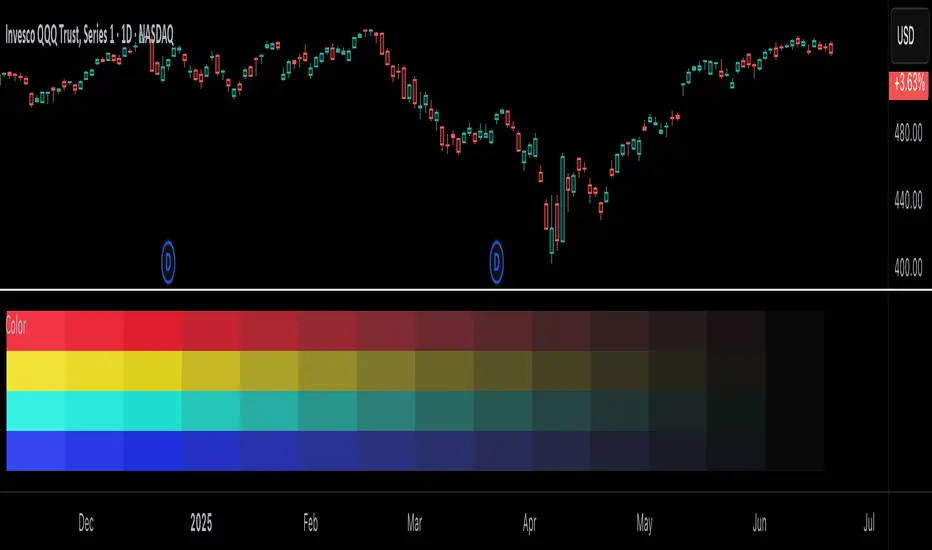
Color█ OVERVIEW
This library is a Pine Script® programming tool for advanced color processing. It provides a comprehensive set of functions for specifying and analyzing colors in various color spaces, mixing and manipulating colors, calculating custom gradients and schemes, detecting contrast, and converting colors to or from hexadecimal strings.
█ CONCEPTS
Color
Color refers to how we interpret light of different wavelengths in the visible spectrum . The colors we see from an object represent the light wavelengths that it reflects, emits, or transmits toward our eyes. Some colors, such as blue and red, correspond directly to parts of the spectrum. Others, such as magenta, arise from a combination of wavelengths to which our minds assign a single color.
The human interpretation of color lends itself to many uses in our world. In the context of financial data analysis, the effective use of color helps transform raw data into insights that users can understand at a glance. For example, colors can categorize series, signal market conditions and sessions, and emphasize patterns or relationships in data.
Color models and spaces
A color model is a general mathematical framework that describes colors using sets of numbers. A color space is an implementation of a specific color model that defines an exact range (gamut) of reproducible colors based on a set of primary colors , a reference white point , and sometimes additional parameters such as viewing conditions.
There are numerous different color spaces — each describing the characteristics of color in unique ways. Different spaces carry different advantages, depending on the application. Below, we provide a brief overview of the concepts underlying the color spaces supported by this library.
RGB
RGB is one of the most well-known color models. It represents color as an additive mixture of three primary colors — red, green, and blue lights — with various intensities. Each cone cell in the human eye responds more strongly to one of the three primaries, and the average person interprets the combination of these lights as a distinct color (e.g., pure red + pure green = yellow).
The sRGB color space is the most common RGB implementation. Developed by HP and Microsoft in the 1990s, sRGB provided a standardized baseline for representing color across CRT monitors of the era, which produced brightness levels that did not increase linearly with the input signal. To match displays and optimize brightness encoding for human sensitivity, sRGB applied a nonlinear transformation to linear RGB signals, often referred to as gamma correction . The result produced more visually pleasing outputs while maintaining a simple encoding. As such, sRGB quickly became a standard for digital color representation across devices and the web. To this day, it remains the default color space for most web-based content.
TradingView charts and Pine Script `color.*` built-ins process color data in sRGB. The red, green, and blue channels range from 0 to 255, where 0 represents no intensity, and 255 represents maximum intensity. Each combination of red, green, and blue values represents a distinct color, resulting in a total of 16,777,216 displayable colors.
CIE XYZ and xyY
The XYZ color space, developed by the International Commission on Illumination (CIE) in 1931, aims to describe all color sensations that a typical human can perceive. It is a cornerstone of color science, forming the basis for many color spaces used today. XYZ, and the derived xyY space, provide a universal representation of color that is not tethered to a particular display. Many widely used color spaces, including sRGB, are defined relative to XYZ or derived from it.
The CIE built the color space based on a series of experiments in which people matched colors they perceived from mixtures of lights. From these experiments, the CIE developed color-matching functions to calculate three components — X, Y, and Z — which together aim to describe a standard observer's response to visible light. X represents a weighted response to light across the color spectrum, with the highest contribution from long wavelengths (e.g., red). Y represents a weighted response to medium wavelengths (e.g., green), and it corresponds to a color's relative luminance (i.e., brightness). Z represents a weighted response to short wavelengths (e.g., blue).
From the XYZ space, the CIE developed the xyY chromaticity space, which separates a color's chromaticity (hue and colorfulness) from luminance. The CIE used this space to define the CIE 1931 chromaticity diagram , which represents the full range of visible colors at a given luminance. In color science and lighting design, xyY is a common means for specifying colors and visualizing the supported ranges of other color spaces.
CIELAB and Oklab
The CIELAB (L*a*b*) color space, derived from XYZ by the CIE in 1976, expresses colors based on opponent process theory. The L* component represents perceived lightness, and the a* and b* components represent the balance between opposing unique colors. The a* value specifies the balance between green and red , and the b* value specifies the balance between blue and yellow .
The primary intention of CIELAB was to provide a perceptually uniform color space, where fixed-size steps through the space correspond to uniform perceived changes in color. Although relatively uniform, the color space has been found to exhibit some non-uniformities, particularly in the blue part of the color spectrum. Regardless, modern applications often use CIELAB to estimate perceived color differences and calculate smooth color gradients.
In 2020, a new LAB-oriented color space, Oklab , was introduced by Björn Ottosson as an attempt to rectify the non-uniformities of other perceptual color spaces. Similar to CIELAB, the L value in Oklab represents perceived lightness, and the a and b values represent the balance between opposing unique colors. Oklab has gained widespread adoption as a perceptual space for color processing, with support in the latest CSS Color specifications and many software applications.
Cylindrical models
A cylindrical-coordinate model transforms an underlying color model, such as RGB or LAB, into an alternative expression of color information that is often more intuitive for the average person to use and understand.
Instead of a mixture of primary colors or opponent pairs, these models represent color as a hue angle on a color wheel , with additional parameters that describe other qualities such as lightness and colorfulness (a general term for concepts like chroma and saturation). In cylindrical-coordinate spaces, users can select a color and modify its lightness or other qualities without altering the hue.
The three most common RGB-based models are HSL (Hue, Saturation, Lightness), HSV (Hue, Saturation, Value), and HWB (Hue, Whiteness, Blackness). All three define hue angles in the same way, but they define colorfulness and lightness differently. Although they are not perceptually uniform, HSL and HSV are commonplace in color pickers and gradients.
For CIELAB and Oklab, the cylindrical-coordinate versions are CIELCh and Oklch , which express color in terms of perceived lightness, chroma, and hue. They offer perceptually uniform alternatives to RGB-based models. These spaces create unique color wheels, and they have more strict definitions of lightness and colorfulness. Oklch is particularly well-suited for generating smooth, perceptual color gradients.
Alpha and transparency
Many color encoding schemes include an alpha channel, representing opacity . Alpha does not help define a color in a color space; it determines how a color interacts with other colors in the display. Opaque colors appear with full intensity on the screen, whereas translucent (semi-opaque) colors blend into the background. Colors with zero opacity are invisible.
In Pine Script, there are two ways to specify a color's alpha:
• Using the `transp` parameter of the built-in `color.*()` functions. The specified value represents transparency (the opposite of opacity), which the functions translate into an alpha value.
• Using eight-digit hexadecimal color codes. The last two digits in the code represent alpha directly.
A process called alpha compositing simulates translucent colors in a display. It creates a single displayed color by mixing the RGB channels of two colors (foreground and background) based on alpha values, giving the illusion of a semi-opaque color placed over another color. For example, a red color with 80% transparency on a black background produces a dark shade of red.
Hexadecimal color codes
A hexadecimal color code (hex code) is a compact representation of an RGB color. It encodes a color's red, green, and blue values into a sequence of hexadecimal ( base-16 ) digits. The digits are numerals ranging from `0` to `9` or letters from `a` (for 10) to `f` (for 15). Each set of two digits represents an RGB channel ranging from `00` (for 0) to `ff` (for 255).
Pine scripts can natively define colors using hex codes in the format `#rrggbbaa`. The first set of two digits represents red, the second represents green, and the third represents blue. The fourth set represents alpha . If unspecified, the value is `ff` (fully opaque). For example, `#ff8b00` and `#ff8b00ff` represent an opaque orange color. The code `#ff8b0033` represents the same color with 80% transparency.
Gradients
A color gradient maps colors to numbers over a given range. Most color gradients represent a continuous path in a specific color space, where each number corresponds to a mix between a starting color and a stopping color. In Pine, coders often use gradients to visualize value intensities in plots and heatmaps, or to add visual depth to fills.
The behavior of a color gradient depends on the mixing method and the chosen color space. Gradients in sRGB usually mix along a straight line between the red, green, and blue coordinates of two colors. In cylindrical spaces such as HSL, a gradient often rotates the hue angle through the color wheel, resulting in more pronounced color transitions.
Color schemes
A color scheme refers to a set of colors for use in aesthetic or functional design. A color scheme usually consists of just a few distinct colors. However, depending on the purpose, a scheme can include many colors.
A user might choose palettes for a color scheme arbitrarily, or generate them algorithmically. There are many techniques for calculating color schemes. A few simple, practical methods are:
• Sampling a set of distinct colors from a color gradient.
• Generating monochromatic variants of a color (i.e., tints, tones, or shades with matching hues).
• Computing color harmonies — such as complements, analogous colors, triads, and tetrads — from a base color.
This library includes functions for all three of these techniques. See below for details.
█ CALCULATIONS AND USE
Hex string conversion
The `getHexString()` function returns a string containing the eight-digit hexadecimal code corresponding to a "color" value or set of sRGB and transparency values. For example, `getHexString(255, 0, 0)` returns the string `"#ff0000ff"`, and `getHexString(color.new(color.red, 80))` returns `"#f2364533"`.
The `hexStringToColor()` function returns the "color" value represented by a string containing a six- or eight-digit hex code. The `hexStringToRGB()` function returns a tuple containing the sRGB and transparency values. For example, `hexStringToColor("#f23645")` returns the same value as color.red .
Programmers can use these functions to parse colors from "string" inputs, perform string-based color calculations, and inspect color data in text outputs such as Pine Logs and tables.
Color space conversion
All other `get*()` functions convert a "color" value or set of sRGB channels into coordinates in a specific color space, with transparency information included. For example, the tuple returned by `getHSL()` includes the color's hue, saturation, lightness, and transparency values.
To convert data from a color space back to colors or sRGB and transparency values, use the corresponding `*toColor()` or `*toRGB()` functions for that space (e.g., `hslToColor()` and `hslToRGB()`).
Programmers can use these conversion functions to process inputs that define colors in different ways, perform advanced color manipulation, design custom gradients, and more.
The color spaces this library supports are:
• sRGB
• Linear RGB (RGB without gamma correction)
• HSL, HSV, and HWB
• CIE XYZ and xyY
• CIELAB and CIELCh
• Oklab and Oklch
Contrast-based calculations
Contrast refers to the difference in luminance or color that makes one color visible against another. This library features two functions for calculating luminance-based contrast and detecting themes.
The `contrastRatio()` function calculates the contrast between two "color" values based on their relative luminance (the Y value from CIE XYZ) using the formula from version 2 of the Web Content Accessibility Guidelines (WCAG) . This function is useful for identifying colors that provide a sufficient brightness difference for legibility.
The `isLightTheme()` function determines whether a specified background color represents a light theme based on its contrast with black and white. Programmers can use this function to define conditional logic that responds differently to light and dark themes.
Color manipulation and harmonies
The `negative()` function calculates the negative (i.e., inverse) of a color by reversing the color's coordinates in either the sRGB or linear RGB color space. This function is useful for calculating high-contrast colors.
The `grayscale()` function calculates a grayscale form of a specified color with the same relative luminance.
The functions `complement()`, `splitComplements()`, `analogousColors()`, `triadicColors()`, `tetradicColors()`, `pentadicColors()`, and `hexadicColors()` calculate color harmonies from a specified source color within a given color space (HSL, CIELCh, or Oklch). The returned harmonious colors represent specific hue rotations around a color wheel formed by the chosen space, with the same defined lightness, saturation or chroma, and transparency.
Color mixing and gradient creation
The `add()` function simulates combining lights of two different colors by additively mixing their linear red, green, and blue components, ignoring transparency by default. Users can calculate a transparency-weighted mixture by setting the `transpWeight` argument to `true`.
The `overlay()` function estimates the color displayed on a TradingView chart when a specific foreground color is over a background color. This function aids in simulating stacked colors and analyzing the effects of transparency.
The `fromGradient()` and `fromMultiStepGradient()` functions calculate colors from gradients in any of the supported color spaces, providing flexible alternatives to the RGB-based color.from_gradient() function. The `fromGradient()` function calculates a color from a single gradient. The `fromMultiStepGradient()` function calculates a color from a piecewise gradient with multiple defined steps. Gradients are useful for heatmaps and for coloring plots or drawings based on value intensities.
Scheme creation
Three functions in this library calculate palettes for custom color schemes. Scripts can use these functions to create responsive color schemes that adjust to calculated values and user inputs.
The `gradientPalette()` function creates an array of colors by sampling a specified number of colors along a gradient from a base color to a target color, in fixed-size steps.
The `monoPalette()` function creates an array containing monochromatic variants (tints, tones, or shades) of a specified base color. Whether the function mixes the color toward white (for tints), a form of gray (for tones), or black (for shades) depends on the `grayLuminance` value. If unspecified, the function automatically chooses the mix behavior with the highest contrast.
The `harmonyPalette()` function creates a matrix of colors. The first column contains the base color and specified harmonies, e.g., triadic colors. The columns that follow contain tints, tones, or shades of the harmonic colors for additional color choices, similar to `monoPalette()`.
█ EXAMPLE CODE
The example code at the end of the script generates and visualizes color schemes by processing user inputs. The code builds the scheme's palette based on the "Base color" input and the additional inputs in the "Settings/Inputs" tab:
• "Palette type" specifies whether the palette uses a custom gradient, monochromatic base color variants, or color harmonies with monochromatic variants.
• "Target color" sets the top color for the "Gradient" palette type.
• The "Gray luminance" inputs determine variation behavior for "Monochromatic" and "Harmony" palette types. If "Auto" is selected, the palette mixes the base color toward white or black based on its brightness. Otherwise, it mixes the color toward the grayscale color with the specified relative luminance (from 0 to 1).
• "Harmony type" specifies the color harmony used in the palette. Each row in the palette corresponds to one of the harmonious colors, starting with the base color.
The code creates a table on the first bar to display the collection of calculated colors. Each cell in the table shows the color's `getHexString()` value in a tooltip for simple inspection.
Look first. Then leap.
█ EXPORTED FUNCTIONS
Below is a complete list of the functions and overloads exported by this library.
getRGB(source)
Retrieves the sRGB red, green, blue, and transparency components of a "color" value.
getHexString(r, g, b, t)
(Overload 1 of 2) Converts a set of sRGB channel values to a string representing the corresponding color's hexadecimal form.
getHexString(source)
(Overload 2 of 2) Converts a "color" value to a string representing the sRGB color's hexadecimal form.
hexStringToRGB(source)
Converts a string representing an sRGB color's hexadecimal form to a set of decimal channel values.
hexStringToColor(source)
Converts a string representing an sRGB color's hexadecimal form to a "color" value.
getLRGB(r, g, b, t)
(Overload 1 of 2) Converts a set of sRGB channel values to a set of linear RGB values with specified transparency information.
getLRGB(source)
(Overload 2 of 2) Retrieves linear RGB channel values and transparency information from a "color" value.
lrgbToRGB(lr, lg, lb, t)
Converts a set of linear RGB channel values to a set of sRGB values with specified transparency information.
lrgbToColor(lr, lg, lb, t)
Converts a set of linear RGB channel values and transparency information to a "color" value.
getHSL(r, g, b, t)
(Overload 1 of 2) Converts a set of sRGB channels to a set of HSL values with specified transparency information.
getHSL(source)
(Overload 2 of 2) Retrieves HSL channel values and transparency information from a "color" value.
hslToRGB(h, s, l, t)
Converts a set of HSL channel values to a set of sRGB values with specified transparency information.
hslToColor(h, s, l, t)
Converts a set of HSL channel values and transparency information to a "color" value.
getHSV(r, g, b, t)
(Overload 1 of 2) Converts a set of sRGB channels to a set of HSV values with specified transparency information.
getHSV(source)
(Overload 2 of 2) Retrieves HSV channel values and transparency information from a "color" value.
hsvToRGB(h, s, v, t)
Converts a set of HSV channel values to a set of sRGB values with specified transparency information.
hsvToColor(h, s, v, t)
Converts a set of HSV channel values and transparency information to a "color" value.
getHWB(r, g, b, t)
(Overload 1 of 2) Converts a set of sRGB channels to a set of HWB values with specified transparency information.
getHWB(source)
(Overload 2 of 2) Retrieves HWB channel values and transparency information from a "color" value.
hwbToRGB(h, w, b, t)
Converts a set of HWB channel values to a set of sRGB values with specified transparency information.
hwbToColor(h, w, b, t)
Converts a set of HWB channel values and transparency information to a "color" value.
getXYZ(r, g, b, t)
(Overload 1 of 2) Converts a set of sRGB channels to a set of XYZ values with specified transparency information.
getXYZ(source)
(Overload 2 of 2) Retrieves XYZ channel values and transparency information from a "color" value.
xyzToRGB(x, y, z, t)
Converts a set of XYZ channel values to a set of sRGB values with specified transparency information
xyzToColor(x, y, z, t)
Converts a set of XYZ channel values and transparency information to a "color" value.
getXYY(r, g, b, t)
(Overload 1 of 2) Converts a set of sRGB channels to a set of xyY values with specified transparency information.
getXYY(source)
(Overload 2 of 2) Retrieves xyY channel values and transparency information from a "color" value.
xyyToRGB(xc, yc, y, t)
Converts a set of xyY channel values to a set of sRGB values with specified transparency information.
xyyToColor(xc, yc, y, t)
Converts a set of xyY channel values and transparency information to a "color" value.
getLAB(r, g, b, t)
(Overload 1 of 2) Converts a set of sRGB channels to a set of CIELAB values with specified transparency information.
getLAB(source)
(Overload 2 of 2) Retrieves CIELAB channel values and transparency information from a "color" value.
labToRGB(l, a, b, t)
Converts a set of CIELAB channel values to a set of sRGB values with specified transparency information.
labToColor(l, a, b, t)
Converts a set of CIELAB channel values and transparency information to a "color" value.
getOKLAB(r, g, b, t)
(Overload 1 of 2) Converts a set of sRGB channels to a set of Oklab values with specified transparency information.
getOKLAB(source)
(Overload 2 of 2) Retrieves Oklab channel values and transparency information from a "color" value.
oklabToRGB(l, a, b, t)
Converts a set of Oklab channel values to a set of sRGB values with specified transparency information.
oklabToColor(l, a, b, t)
Converts a set of Oklab channel values and transparency information to a "color" value.
getLCH(r, g, b, t)
(Overload 1 of 2) Converts a set of sRGB channels to a set of CIELCh values with specified transparency information.
getLCH(source)
(Overload 2 of 2) Retrieves CIELCh channel values and transparency information from a "color" value.
lchToRGB(l, c, h, t)
Converts a set of CIELCh channel values to a set of sRGB values with specified transparency information.
lchToColor(l, c, h, t)
Converts a set of CIELCh channel values and transparency information to a "color" value.
getOKLCH(r, g, b, t)
(Overload 1 of 2) Converts a set of sRGB channels to a set of Oklch values with specified transparency information.
getOKLCH(source)
(Overload 2 of 2) Retrieves Oklch channel values and transparency information from a "color" value.
oklchToRGB(l, c, h, t)
Converts a set of Oklch channel values to a set of sRGB values with specified transparency information.
oklchToColor(l, c, h, t)
Converts a set of Oklch channel values and transparency information to a "color" value.
contrastRatio(value1, value2)
Calculates the contrast ratio between two colors values based on the formula from version 2 of the Web Content Accessibility Guidelines (WCAG).
isLightTheme(source)
Detects whether a background color represents a light theme or dark theme, based on the amount of contrast between the color and the white and black points.
grayscale(source)
Calculates the grayscale version of a color with the same relative luminance (i.e., brightness).
negative(source, colorSpace)
Calculates the negative (i.e., inverted) form of a specified color.
complement(source, colorSpace)
Calculates the complementary color for a `source` color using a cylindrical color space.
analogousColors(source, colorSpace)
Calculates the analogous colors for a `source` color using a cylindrical color space.
splitComplements(source, colorSpace)
Calculates the split-complementary colors for a `source` color using a cylindrical color space.
triadicColors(source, colorSpace)
Calculates the two triadic colors for a `source` color using a cylindrical color space.
tetradicColors(source, colorSpace, square)
Calculates the three square or rectangular tetradic colors for a `source` color using a cylindrical color space.
pentadicColors(source, colorSpace)
Calculates the four pentadic colors for a `source` color using a cylindrical color space.
hexadicColors(source, colorSpace)
Calculates the five hexadic colors for a `source` color using a cylindrical color space.
add(value1, value2, transpWeight)
Additively mixes two "color" values, with optional transparency weighting.
overlay(fg, bg)
Estimates the resulting color that appears on the chart when placing one color over another.
fromGradient(value, bottomValue, topValue, bottomColor, topColor, colorSpace)
Calculates the gradient color that corresponds to a specific value based on a defined value range and color space.
fromMultiStepGradient(value, steps, colors, colorSpace)
Calculates a multi-step gradient color that corresponds to a specific value based on an array of step points, an array of corresponding colors, and a color space.
gradientPalette(baseColor, stopColor, steps, strength, model)
Generates a palette from a gradient between two base colors.
monoPalette(baseColor, grayLuminance, variations, strength, colorSpace)
Generates a monochromatic palette from a specified base color.
harmonyPalette(baseColor, harmonyType, grayLuminance, variations, strength, colorSpace)
Generates a palette consisting of harmonious base colors and their monochromatic variants.
Tensor Market Analysis Engine (TMAE)# Tensor Market Analysis Engine (TMAE)
## Advanced Multi-Dimensional Mathematical Analysis System
*Where Quantum Mathematics Meets Market Structure*
---
## 🎓 THEORETICAL FOUNDATION
The Tensor Market Analysis Engine represents a revolutionary synthesis of three cutting-edge mathematical frameworks that have never before been combined for comprehensive market analysis. This indicator transcends traditional technical analysis by implementing advanced mathematical concepts from quantum mechanics, information theory, and fractal geometry.
### 🌊 Multi-Dimensional Volatility with Jump Detection
**Hawkes Process Implementation:**
The TMAE employs a sophisticated Hawkes process approximation for detecting self-exciting market jumps. Unlike traditional volatility measures that treat price movements as independent events, the Hawkes process recognizes that market shocks cluster and exhibit memory effects.
**Mathematical Foundation:**
```
Intensity λ(t) = μ + Σ α(t - Tᵢ)
```
Where market jumps at times Tᵢ increase the probability of future jumps through the decay function α, controlled by the Hawkes Decay parameter (0.5-0.99).
**Mahalanobis Distance Calculation:**
The engine calculates volatility jumps using multi-dimensional Mahalanobis distance across up to 5 volatility dimensions:
- **Dimension 1:** Price volatility (standard deviation of returns)
- **Dimension 2:** Volume volatility (normalized volume fluctuations)
- **Dimension 3:** Range volatility (high-low spread variations)
- **Dimension 4:** Correlation volatility (price-volume relationship changes)
- **Dimension 5:** Microstructure volatility (intrabar positioning analysis)
This creates a volatility state vector that captures market behavior impossible to detect with traditional single-dimensional approaches.
### 📐 Hurst Exponent Regime Detection
**Fractal Market Hypothesis Integration:**
The TMAE implements advanced Rescaled Range (R/S) analysis to calculate the Hurst exponent in real-time, providing dynamic regime classification:
- **H > 0.6:** Trending (persistent) markets - momentum strategies optimal
- **H < 0.4:** Mean-reverting (anti-persistent) markets - contrarian strategies optimal
- **H ≈ 0.5:** Random walk markets - breakout strategies preferred
**Adaptive R/S Analysis:**
Unlike static implementations, the TMAE uses adaptive windowing that adjusts to market conditions:
```
H = log(R/S) / log(n)
```
Where R is the range of cumulative deviations and S is the standard deviation over period n.
**Dynamic Regime Classification:**
The system employs hysteresis to prevent regime flipping, requiring sustained Hurst values before regime changes are confirmed. This prevents false signals during transitional periods.
### 🔄 Transfer Entropy Analysis
**Information Flow Quantification:**
Transfer entropy measures the directional flow of information between price and volume, revealing lead-lag relationships that indicate future price movements:
```
TE(X→Y) = Σ p(yₜ₊₁, yₜ, xₜ) log
```
**Causality Detection:**
- **Volume → Price:** Indicates accumulation/distribution phases
- **Price → Volume:** Suggests retail participation or momentum chasing
- **Balanced Flow:** Market equilibrium or transition periods
The system analyzes multiple lag periods (2-20 bars) to capture both immediate and structural information flows.
---
## 🔧 COMPREHENSIVE INPUT SYSTEM
### Core Parameters Group
**Primary Analysis Window (10-100, Default: 50)**
The fundamental lookback period affecting all calculations. Optimization by timeframe:
- **1-5 minute charts:** 20-30 (rapid adaptation to micro-movements)
- **15 minute-1 hour:** 30-50 (balanced responsiveness and stability)
- **4 hour-daily:** 50-100 (smooth signals, reduced noise)
- **Asset-specific:** Cryptocurrency 20-35, Stocks 35-50, Forex 40-60
**Signal Sensitivity (0.1-2.0, Default: 0.7)**
Master control affecting all threshold calculations:
- **Conservative (0.3-0.6):** High-quality signals only, fewer false positives
- **Balanced (0.7-1.0):** Optimal risk-reward ratio for most trading styles
- **Aggressive (1.1-2.0):** Maximum signal frequency, requires careful filtering
**Signal Generation Mode:**
- **Aggressive:** Any component signals (highest frequency)
- **Confluence:** 2+ components agree (balanced approach)
- **Conservative:** All 3 components align (highest quality)
### Volatility Jump Detection Group
**Volatility Dimensions (2-5, Default: 3)**
Determines the mathematical space complexity:
- **2D:** Price + Volume volatility (suitable for clean markets)
- **3D:** + Range volatility (optimal for most conditions)
- **4D:** + Correlation volatility (advanced multi-asset analysis)
- **5D:** + Microstructure volatility (maximum sensitivity)
**Jump Detection Threshold (1.5-4.0σ, Default: 3.0σ)**
Standard deviations required for volatility jump classification:
- **Cryptocurrency:** 2.0-2.5σ (naturally volatile)
- **Stock Indices:** 2.5-3.0σ (moderate volatility)
- **Forex Major Pairs:** 3.0-3.5σ (typically stable)
- **Commodities:** 2.0-3.0σ (varies by commodity)
**Jump Clustering Decay (0.5-0.99, Default: 0.85)**
Hawkes process memory parameter:
- **0.5-0.7:** Fast decay (jumps treated as independent)
- **0.8-0.9:** Moderate clustering (realistic market behavior)
- **0.95-0.99:** Strong clustering (crisis/event-driven markets)
### Hurst Exponent Analysis Group
**Calculation Method Options:**
- **Classic R/S:** Original Rescaled Range (fast, simple)
- **Adaptive R/S:** Dynamic windowing (recommended for trading)
- **DFA:** Detrended Fluctuation Analysis (best for noisy data)
**Trending Threshold (0.55-0.8, Default: 0.60)**
Hurst value defining persistent market behavior:
- **0.55-0.60:** Weak trend persistence
- **0.65-0.70:** Clear trending behavior
- **0.75-0.80:** Strong momentum regimes
**Mean Reversion Threshold (0.2-0.45, Default: 0.40)**
Hurst value defining anti-persistent behavior:
- **0.35-0.45:** Weak mean reversion
- **0.25-0.35:** Clear ranging behavior
- **0.15-0.25:** Strong reversion tendency
### Transfer Entropy Parameters Group
**Information Flow Analysis:**
- **Price-Volume:** Classic flow analysis for accumulation/distribution
- **Price-Volatility:** Risk flow analysis for sentiment shifts
- **Multi-Timeframe:** Cross-timeframe causality detection
**Maximum Lag (2-20, Default: 5)**
Causality detection window:
- **2-5 bars:** Immediate causality (scalping)
- **5-10 bars:** Short-term flow (day trading)
- **10-20 bars:** Structural flow (swing trading)
**Significance Threshold (0.05-0.3, Default: 0.15)**
Minimum entropy for signal generation:
- **0.05-0.10:** Detect subtle information flows
- **0.10-0.20:** Clear causality only
- **0.20-0.30:** Very strong flows only
---
## 🎨 ADVANCED VISUAL SYSTEM
### Tensor Volatility Field Visualization
**Five-Layer Resonance Bands:**
The tensor field creates dynamic support/resistance zones that expand and contract based on mathematical field strength:
- **Core Layer (Purple):** Primary tensor field with highest intensity
- **Layer 2 (Neutral):** Secondary mathematical resonance
- **Layer 3 (Info Blue):** Tertiary harmonic frequencies
- **Layer 4 (Warning Gold):** Outer field boundaries
- **Layer 5 (Success Green):** Maximum field extension
**Field Strength Calculation:**
```
Field Strength = min(3.0, Mahalanobis Distance × Tensor Intensity)
```
The field amplitude adjusts to ATR and mathematical distance, creating dynamic zones that respond to market volatility.
**Radiation Line Network:**
During active tensor states, the system projects directional radiation lines showing field energy distribution:
- **8 Directional Rays:** Complete angular coverage
- **Tapering Segments:** Progressive transparency for natural visual flow
- **Pulse Effects:** Enhanced visualization during volatility jumps
### Dimensional Portal System
**Portal Mathematics:**
Dimensional portals visualize regime transitions using category theory principles:
- **Green Portals (◉):** Trending regime detection (appear below price for support)
- **Red Portals (◎):** Mean-reverting regime (appear above price for resistance)
- **Yellow Portals (○):** Random walk regime (neutral positioning)
**Tensor Trail Effects:**
Each portal generates 8 trailing particles showing mathematical momentum:
- **Large Particles (●):** Strong mathematical signal
- **Medium Particles (◦):** Moderate signal strength
- **Small Particles (·):** Weak signal continuation
- **Micro Particles (˙):** Signal dissipation
### Information Flow Streams
**Particle Stream Visualization:**
Transfer entropy creates flowing particle streams indicating information direction:
- **Upward Streams:** Volume leading price (accumulation phases)
- **Downward Streams:** Price leading volume (distribution phases)
- **Stream Density:** Proportional to information flow strength
**15-Particle Evolution:**
Each stream contains 15 particles with progressive sizing and transparency, creating natural flow visualization that makes information transfer immediately apparent.
### Fractal Matrix Grid System
**Multi-Timeframe Fractal Levels:**
The system calculates and displays fractal highs/lows across five Fibonacci periods:
- **8-Period:** Short-term fractal structure
- **13-Period:** Intermediate-term patterns
- **21-Period:** Primary swing levels
- **34-Period:** Major structural levels
- **55-Period:** Long-term fractal boundaries
**Triple-Layer Visualization:**
Each fractal level uses three-layer rendering:
- **Shadow Layer:** Widest, darkest foundation (width 5)
- **Glow Layer:** Medium white core line (width 3)
- **Tensor Layer:** Dotted mathematical overlay (width 1)
**Intelligent Labeling System:**
Smart spacing prevents label overlap using ATR-based minimum distances. Labels include:
- **Fractal Period:** Time-based identification
- **Topological Class:** Mathematical complexity rating (0, I, II, III)
- **Price Level:** Exact fractal price
- **Mahalanobis Distance:** Current mathematical field strength
- **Hurst Exponent:** Current regime classification
- **Anomaly Indicators:** Visual strength representations (○ ◐ ● ⚡)
### Wick Pressure Analysis
**Rejection Level Mathematics:**
The system analyzes candle wick patterns to project future pressure zones:
- **Upper Wick Analysis:** Identifies selling pressure and resistance zones
- **Lower Wick Analysis:** Identifies buying pressure and support zones
- **Pressure Projection:** Extends lines forward based on mathematical probability
**Multi-Layer Glow Effects:**
Wick pressure lines use progressive transparency (1-8 layers) creating natural glow effects that make pressure zones immediately visible without cluttering the chart.
### Enhanced Regime Background
**Dynamic Intensity Mapping:**
Background colors reflect mathematical regime strength:
- **Deep Transparency (98% alpha):** Subtle regime indication
- **Pulse Intensity:** Based on regime strength calculation
- **Color Coding:** Green (trending), Red (mean-reverting), Neutral (random)
**Smoothing Integration:**
Regime changes incorporate 10-bar smoothing to prevent background flicker while maintaining responsiveness to genuine regime shifts.
### Color Scheme System
**Six Professional Themes:**
- **Dark (Default):** Professional trading environment optimization
- **Light:** High ambient light conditions
- **Classic:** Traditional technical analysis appearance
- **Neon:** High-contrast visibility for active trading
- **Neutral:** Minimal distraction focus
- **Bright:** Maximum visibility for complex setups
Each theme maintains mathematical accuracy while optimizing visual clarity for different trading environments and personal preferences.
---
## 📊 INSTITUTIONAL-GRADE DASHBOARD
### Tensor Field Status Section
**Field Strength Display:**
Real-time Mahalanobis distance calculation with dynamic emoji indicators:
- **⚡ (Lightning):** Extreme field strength (>1.5× threshold)
- **● (Solid Circle):** Strong field activity (>1.0× threshold)
- **○ (Open Circle):** Normal field state
**Signal Quality Rating:**
Democratic algorithm assessment:
- **ELITE:** All 3 components aligned (highest probability)
- **STRONG:** 2 components aligned (good probability)
- **GOOD:** 1 component active (moderate probability)
- **WEAK:** No clear component signals
**Threshold and Anomaly Monitoring:**
- **Threshold Display:** Current mathematical threshold setting
- **Anomaly Level (0-100%):** Combined volatility and volume spike measurement
- **>70%:** High anomaly (red warning)
- **30-70%:** Moderate anomaly (orange caution)
- **<30%:** Normal conditions (green confirmation)
### Tensor State Analysis Section
**Mathematical State Classification:**
- **↑ BULL (Tensor State +1):** Trending regime with bullish bias
- **↓ BEAR (Tensor State -1):** Mean-reverting regime with bearish bias
- **◈ SUPER (Tensor State 0):** Random walk regime (neutral)
**Visual State Gauge:**
Five-circle progression showing tensor field polarity:
- **🟢🟢🟢⚪⚪:** Strong bullish mathematical alignment
- **⚪⚪🟡⚪⚪:** Neutral/transitional state
- **⚪⚪🔴🔴🔴:** Strong bearish mathematical alignment
**Trend Direction and Phase Analysis:**
- **📈 BULL / 📉 BEAR / ➡️ NEUTRAL:** Primary trend classification
- **🌪️ CHAOS:** Extreme information flow (>2.0 flow strength)
- **⚡ ACTIVE:** Strong information flow (1.0-2.0 flow strength)
- **😴 CALM:** Low information flow (<1.0 flow strength)
### Trading Signals Section
**Real-Time Signal Status:**
- **🟢 ACTIVE / ⚪ INACTIVE:** Long signal availability
- **🔴 ACTIVE / ⚪ INACTIVE:** Short signal availability
- **Components (X/3):** Active algorithmic components
- **Mode Display:** Current signal generation mode
**Signal Strength Visualization:**
Color-coded component count:
- **Green:** 3/3 components (maximum confidence)
- **Aqua:** 2/3 components (good confidence)
- **Orange:** 1/3 components (moderate confidence)
- **Gray:** 0/3 components (no signals)
### Performance Metrics Section
**Win Rate Monitoring:**
Estimated win rates based on signal quality with emoji indicators:
- **🔥 (Fire):** ≥60% estimated win rate
- **👍 (Thumbs Up):** 45-59% estimated win rate
- **⚠️ (Warning):** <45% estimated win rate
**Mathematical Metrics:**
- **Hurst Exponent:** Real-time fractal dimension (0.000-1.000)
- **Information Flow:** Volume/price leading indicators
- **📊 VOL:** Volume leading price (accumulation/distribution)
- **💰 PRICE:** Price leading volume (momentum/speculation)
- **➖ NONE:** Balanced information flow
- **Volatility Classification:**
- **🔥 HIGH:** Above 1.5× jump threshold
- **📊 NORM:** Normal volatility range
- **😴 LOW:** Below 0.5× jump threshold
### Market Structure Section (Large Dashboard)
**Regime Classification:**
- **📈 TREND:** Hurst >0.6, momentum strategies optimal
- **🔄 REVERT:** Hurst <0.4, contrarian strategies optimal
- **🎲 RANDOM:** Hurst ≈0.5, breakout strategies preferred
**Mathematical Field Analysis:**
- **Dimensions:** Current volatility space complexity (2D-5D)
- **Hawkes λ (Lambda):** Self-exciting jump intensity (0.00-1.00)
- **Jump Status:** 🚨 JUMP (active) / ✅ NORM (normal)
### Settings Summary Section (Large Dashboard)
**Active Configuration Display:**
- **Sensitivity:** Current master sensitivity setting
- **Lookback:** Primary analysis window
- **Theme:** Active color scheme
- **Method:** Hurst calculation method (Classic R/S, Adaptive R/S, DFA)
**Dashboard Sizing Options:**
- **Small:** Essential metrics only (mobile/small screens)
- **Normal:** Balanced information density (standard desktop)
- **Large:** Maximum detail (multi-monitor setups)
**Position Options:**
- **Top Right:** Standard placement (avoids price action)
- **Top Left:** Wide chart optimization
- **Bottom Right:** Recent price focus (scalping)
- **Bottom Left:** Maximum price visibility (swing trading)
---
## 🎯 SIGNAL GENERATION LOGIC
### Multi-Component Convergence System
**Component Signal Architecture:**
The TMAE generates signals through sophisticated component analysis rather than simple threshold crossing:
**Volatility Component:**
- **Jump Detection:** Mahalanobis distance threshold breach
- **Hawkes Intensity:** Self-exciting process activation (>0.2)
- **Multi-dimensional:** Considers all volatility dimensions simultaneously
**Hurst Regime Component:**
- **Trending Markets:** Price above SMA-20 with positive momentum
- **Mean-Reverting Markets:** Price at Bollinger Band extremes
- **Random Markets:** Bollinger squeeze breakouts with directional confirmation
**Transfer Entropy Component:**
- **Volume Leadership:** Information flow from volume to price
- **Volume Spike:** Volume 110%+ above 20-period average
- **Flow Significance:** Above entropy threshold with directional bias
### Democratic Signal Weighting
**Signal Mode Implementation:**
- **Aggressive Mode:** Any single component triggers signal
- **Confluence Mode:** Minimum 2 components must agree
- **Conservative Mode:** All 3 components must align
**Momentum Confirmation:**
All signals require momentum confirmation:
- **Long Signals:** RSI >50 AND price >EMA-9
- **Short Signals:** RSI <50 AND price 0.6):**
- **Increase Sensitivity:** Catch momentum continuation
- **Lower Mean Reversion Threshold:** Avoid counter-trend signals
- **Emphasize Volume Leadership:** Institutional accumulation/distribution
- **Tensor Field Focus:** Use expansion for trend continuation
- **Signal Mode:** Aggressive or Confluence for trend following
**Range-Bound Markets (Hurst <0.4):**
- **Decrease Sensitivity:** Avoid false breakouts
- **Lower Trending Threshold:** Quick regime recognition
- **Focus on Price Leadership:** Retail sentiment extremes
- **Fractal Grid Emphasis:** Support/resistance trading
- **Signal Mode:** Conservative for high-probability reversals
**Volatile Markets (High Jump Frequency):**
- **Increase Hawkes Decay:** Recognize event clustering
- **Higher Jump Threshold:** Avoid noise signals
- **Maximum Dimensions:** Capture full volatility complexity
- **Reduce Position Sizing:** Risk management adaptation
- **Enhanced Visuals:** Maximum information for rapid decisions
**Low Volatility Markets (Low Jump Frequency):**
- **Decrease Jump Threshold:** Capture subtle movements
- **Lower Hawkes Decay:** Treat moves as independent
- **Reduce Dimensions:** Simplify analysis
- **Increase Position Sizing:** Capitalize on compressed volatility
- **Minimal Visuals:** Reduce distraction in quiet markets
---
## 🚀 ADVANCED TRADING STRATEGIES
### The Mathematical Convergence Method
**Entry Protocol:**
1. **Fractal Grid Approach:** Monitor price approaching significant fractal levels
2. **Tensor Field Confirmation:** Verify field expansion supporting direction
3. **Portal Signal:** Wait for dimensional portal appearance
4. **ELITE/STRONG Quality:** Only trade highest quality mathematical signals
5. **Component Consensus:** Confirm 2+ components agree in Confluence mode
**Example Implementation:**
- Price approaching 21-period fractal high
- Tensor field expanding upward (bullish mathematical alignment)
- Green portal appears below price (trending regime confirmation)
- ELITE quality signal with 3/3 components active
- Enter long position with stop below fractal level
**Risk Management:**
- **Stop Placement:** Below/above fractal level that generated signal
- **Position Sizing:** Based on Mahalanobis distance (higher distance = smaller size)
- **Profit Targets:** Next fractal level or tensor field resistance
### The Regime Transition Strategy
**Regime Change Detection:**
1. **Monitor Hurst Exponent:** Watch for persistent moves above/below thresholds
2. **Portal Color Change:** Regime transitions show different portal colors
3. **Background Intensity:** Increasing regime background intensity
4. **Mathematical Confirmation:** Wait for regime confirmation (hysteresis)
**Trading Implementation:**
- **Trending Transitions:** Trade momentum breakouts, follow trend
- **Mean Reversion Transitions:** Trade range boundaries, fade extremes
- **Random Transitions:** Trade breakouts with tight stops
**Advanced Techniques:**
- **Multi-Timeframe:** Confirm regime on higher timeframe
- **Early Entry:** Enter on regime transition rather than confirmation
- **Regime Strength:** Larger positions during strong regime signals
### The Information Flow Momentum Strategy
**Flow Detection Protocol:**
1. **Monitor Transfer Entropy:** Watch for significant information flow shifts
2. **Volume Leadership:** Strong edge when volume leads price
3. **Flow Acceleration:** Increasing flow strength indicates momentum
4. **Directional Confirmation:** Ensure flow aligns with intended trade direction
**Entry Signals:**
- **Volume → Price Flow:** Enter during accumulation/distribution phases
- **Price → Volume Flow:** Enter on momentum confirmation breaks
- **Flow Reversal:** Counter-trend entries when flow reverses
**Optimization:**
- **Scalping:** Use immediate flow detection (2-5 bar lag)
- **Swing Trading:** Use structural flow (10-20 bar lag)
- **Multi-Asset:** Compare flow between correlated assets
### The Tensor Field Expansion Strategy
**Field Mathematics:**
The tensor field expansion indicates mathematical pressure building in market structure:
**Expansion Phases:**
1. **Compression:** Field contracts, volatility decreases
2. **Tension Building:** Mathematical pressure accumulates
3. **Expansion:** Field expands rapidly with directional movement
4. **Resolution:** Field stabilizes at new equilibrium
**Trading Applications:**
- **Compression Trading:** Prepare for breakout during field contraction
- **Expansion Following:** Trade direction of field expansion
- **Reversion Trading:** Fade extreme field expansion
- **Multi-Dimensional:** Consider all field layers for confirmation
### The Hawkes Process Event Strategy
**Self-Exciting Jump Trading:**
Understanding that market shocks cluster and create follow-on opportunities:
**Jump Sequence Analysis:**
1. **Initial Jump:** First volatility jump detected
2. **Clustering Phase:** Hawkes intensity remains elevated
3. **Follow-On Opportunities:** Additional jumps more likely
4. **Decay Period:** Intensity gradually decreases
**Implementation:**
- **Jump Confirmation:** Wait for mathematical jump confirmation
- **Direction Assessment:** Use other components for direction
- **Clustering Trades:** Trade subsequent moves during high intensity
- **Decay Exit:** Exit positions as Hawkes intensity decays
### The Fractal Confluence System
**Multi-Timeframe Fractal Analysis:**
Combining fractal levels across different periods for high-probability zones:
**Confluence Zones:**
- **Double Confluence:** 2 fractal levels align
- **Triple Confluence:** 3+ fractal levels cluster
- **Mathematical Confirmation:** Tensor field supports the level
- **Information Flow:** Transfer entropy confirms direction
**Trading Protocol:**
1. **Identify Confluence:** Find 2+ fractal levels within 1 ATR
2. **Mathematical Support:** Verify tensor field alignment
3. **Signal Quality:** Wait for STRONG or ELITE signal
4. **Risk Definition:** Use fractal level for stop placement
5. **Profit Targeting:** Next major fractal confluence zone
---
## ⚠️ COMPREHENSIVE RISK MANAGEMENT
### Mathematical Position Sizing
**Mahalanobis Distance Integration:**
Position size should inversely correlate with mathematical field strength:
```
Position Size = Base Size × (Threshold / Mahalanobis Distance)
```
**Risk Scaling Matrix:**
- **Low Field Strength (<2.0):** Standard position sizing
- **Moderate Field Strength (2.0-3.0):** 75% position sizing
- **High Field Strength (3.0-4.0):** 50% position sizing
- **Extreme Field Strength (>4.0):** 25% position sizing or no trade
### Signal Quality Risk Adjustment
**Quality-Based Position Sizing:**
- **ELITE Signals:** 100% of planned position size
- **STRONG Signals:** 75% of planned position size
- **GOOD Signals:** 50% of planned position size
- **WEAK Signals:** No position or paper trading only
**Component Agreement Scaling:**
- **3/3 Components:** Full position size
- **2/3 Components:** 75% position size
- **1/3 Components:** 50% position size or skip trade
### Regime-Adaptive Risk Management
**Trending Market Risk:**
- **Wider Stops:** Allow for trend continuation
- **Trend Following:** Trade with regime direction
- **Higher Position Size:** Trend probability advantage
- **Momentum Stops:** Trail stops based on momentum indicators
**Mean-Reverting Market Risk:**
- **Tighter Stops:** Quick exits on trend continuation
- **Contrarian Positioning:** Trade against extremes
- **Smaller Position Size:** Higher reversal failure rate
- **Level-Based Stops:** Use fractal levels for stops
**Random Market Risk:**
- **Breakout Focus:** Trade only clear breakouts
- **Tight Initial Stops:** Quick exit if breakout fails
- **Reduced Frequency:** Skip marginal setups
- **Range-Based Targets:** Profit targets at range boundaries
### Volatility-Adaptive Risk Controls
**High Volatility Periods:**
- **Reduced Position Size:** Account for wider price swings
- **Wider Stops:** Avoid noise-based exits
- **Lower Frequency:** Skip marginal setups
- **Faster Exits:** Take profits more quickly
**Low Volatility Periods:**
- **Standard Position Size:** Normal risk parameters
- **Tighter Stops:** Take advantage of compressed ranges
- **Higher Frequency:** Trade more setups
- **Extended Targets:** Allow for compressed volatility expansion
### Multi-Timeframe Risk Alignment
**Higher Timeframe Trend:**
- **With Trend:** Standard or increased position size
- **Against Trend:** Reduced position size or skip
- **Neutral Trend:** Standard position size with tight management
**Risk Hierarchy:**
1. **Primary:** Current timeframe signal quality
2. **Secondary:** Higher timeframe trend alignment
3. **Tertiary:** Mathematical field strength
4. **Quaternary:** Market regime classification
---
## 📚 EDUCATIONAL VALUE AND MATHEMATICAL CONCEPTS
### Advanced Mathematical Concepts
**Tensor Analysis in Markets:**
The TMAE introduces traders to tensor analysis, a branch of mathematics typically reserved for physics and advanced engineering. Tensors provide a framework for understanding multi-dimensional market relationships that scalar and vector analysis cannot capture.
**Information Theory Applications:**
Transfer entropy implementation teaches traders about information flow in markets, a concept from information theory that quantifies directional causality between variables. This provides intuition about market microstructure and participant behavior.
**Fractal Geometry in Trading:**
The Hurst exponent calculation exposes traders to fractal geometry concepts, helping understand that markets exhibit self-similar patterns across multiple timeframes. This mathematical insight transforms how traders view market structure.
**Stochastic Process Theory:**
The Hawkes process implementation introduces concepts from stochastic process theory, specifically self-exciting point processes. This provides mathematical framework for understanding why market events cluster and exhibit memory effects.
### Learning Progressive Complexity
**Beginner Mathematical Concepts:**
- **Volatility Dimensions:** Understanding multi-dimensional analysis
- **Regime Classification:** Learning market personality types
- **Signal Democracy:** Algorithmic consensus building
- **Visual Mathematics:** Interpreting mathematical concepts visually
**Intermediate Mathematical Applications:**
- **Mahalanobis Distance:** Statistical distance in multi-dimensional space
- **Rescaled Range Analysis:** Fractal dimension measurement
- **Information Entropy:** Quantifying uncertainty and causality
- **Field Theory:** Understanding mathematical fields in market context
**Advanced Mathematical Integration:**
- **Tensor Field Dynamics:** Multi-dimensional market force analysis
- **Stochastic Self-Excitation:** Event clustering and memory effects
- **Categorical Composition:** Mathematical signal combination theory
- **Topological Market Analysis:** Understanding market shape and connectivity
### Practical Mathematical Intuition
**Developing Market Mathematics Intuition:**
The TMAE serves as a bridge between abstract mathematical concepts and practical trading applications. Traders develop intuitive understanding of:
- **How markets exhibit mathematical structure beneath apparent randomness**
- **Why multi-dimensional analysis reveals patterns invisible to single-variable approaches**
- **How information flows through markets in measurable, predictable ways**
- **Why mathematical models provide probabilistic edges rather than certainties**
---
## 🔬 IMPLEMENTATION AND OPTIMIZATION
### Getting Started Protocol
**Phase 1: Observation (Week 1)**
1. **Apply with defaults:** Use standard settings on your primary trading timeframe
2. **Study visual elements:** Learn to interpret tensor fields, portals, and streams
3. **Monitor dashboard:** Observe how metrics change with market conditions
4. **No trading:** Focus entirely on pattern recognition and understanding
**Phase 2: Pattern Recognition (Week 2-3)**
1. **Identify signal patterns:** Note what market conditions produce different signal qualities
2. **Regime correlation:** Observe how Hurst regimes affect signal performance
3. **Visual confirmation:** Learn to read tensor field expansion and portal signals
4. **Component analysis:** Understand which components drive signals in different markets
**Phase 3: Parameter Optimization (Week 4-5)**
1. **Asset-specific tuning:** Adjust parameters for your specific trading instrument
2. **Timeframe optimization:** Fine-tune for your preferred trading timeframe
3. **Sensitivity adjustment:** Balance signal frequency with quality
4. **Visual customization:** Optimize colors and intensity for your trading environment
**Phase 4: Live Implementation (Week 6+)**
1. **Paper trading:** Test signals with hypothetical trades
2. **Small position sizing:** Begin with minimal risk during learning phase
3. **Performance tracking:** Monitor actual vs. expected signal performance
4. **Continuous optimization:** Refine settings based on real performance data
### Performance Monitoring System
**Signal Quality Tracking:**
- **ELITE Signal Win Rate:** Track highest quality signals separately
- **Component Performance:** Monitor which components provide best signals
- **Regime Performance:** Analyze performance across different market regimes
- **Timeframe Analysis:** Compare performance across different session times
**Mathematical Metric Correlation:**
- **Field Strength vs. Performance:** Higher field strength should correlate with better performance
- **Component Agreement vs. Win Rate:** More component agreement should improve win rates
- **Regime Alignment vs. Success:** Trading with mathematical regime should outperform
### Continuous Optimization Process
**Monthly Review Protocol:**
1. **Performance Analysis:** Review win rates, profit factors, and maximum drawdown
2. **Parameter Assessment:** Evaluate if current settings remain optimal
3. **Market Adaptation:** Adjust for changes in market character or volatility
4. **Component Weighting:** Consider if certain components should receive more/less emphasis
**Quarterly Deep Analysis:**
1. **Mathematical Model Validation:** Verify that mathematical relationships remain valid
2. **Regime Distribution:** Analyze time spent in different market regimes
3. **Signal Evolution:** Track how signal characteristics change over time
4. **Correlation Analysis:** Monitor correlations between different mathematical components
---
## 🌟 UNIQUE INNOVATIONS AND CONTRIBUTIONS
### Revolutionary Mathematical Integration
**First-Ever Implementations:**
1. **Multi-Dimensional Volatility Tensor:** First indicator to implement true tensor analysis for market volatility
2. **Real-Time Hawkes Process:** First trading implementation of self-exciting point processes
3. **Transfer Entropy Trading Signals:** First practical application of information theory for trade generation
4. **Democratic Component Voting:** First algorithmic consensus system for signal generation
5. **Fractal-Projected Signal Quality:** First system to predict signal quality at future price levels
### Advanced Visualization Innovations
**Mathematical Visualization Breakthroughs:**
- **Tensor Field Radiation:** Visual representation of mathematical field energy
- **Dimensional Portal System:** Category theory visualization for regime transitions
- **Information Flow Streams:** Real-time visual display of market information transfer
- **Multi-Layer Fractal Grid:** Intelligent spacing and projection system
- **Regime Intensity Mapping:** Dynamic background showing mathematical regime strength
### Practical Trading Innovations
**Trading System Advances:**
- **Quality-Weighted Signal Generation:** Signals rated by mathematical confidence
- **Regime-Adaptive Strategy Selection:** Automatic strategy optimization based on market personality
- **Anti-Spam Signal Protection:** Mathematical prevention of signal clustering
- **Component Performance Tracking:** Real-time monitoring of algorithmic component success
- **Field-Strength Position Sizing:** Mathematical volatility integration for risk management
---
## ⚖️ RESPONSIBLE USAGE AND LIMITATIONS
### Mathematical Model Limitations
**Understanding Model Boundaries:**
While the TMAE implements sophisticated mathematical concepts, traders must understand fundamental limitations:
- **Markets Are Not Purely Mathematical:** Human psychology, news events, and fundamental factors create unpredictable elements
- **Past Performance Limitations:** Mathematical relationships that worked historically may not persist indefinitely
- **Model Risk:** Complex models can fail during unprecedented market conditions
- **Overfitting Potential:** Highly optimized parameters may not generalize to future market conditions
### Proper Implementation Guidelines
**Risk Management Requirements:**
- **Never Risk More Than 2% Per Trade:** Regardless of signal quality
- **Diversification Mandatory:** Don't rely solely on mathematical signals
- **Position Sizing Discipline:** Use mathematical field strength for sizing, not confidence
- **Stop Loss Non-Negotiable:** Every trade must have predefined risk parameters
**Realistic Expectations:**
- **Mathematical Edge, Not Certainty:** The indicator provides probabilistic advantages, not guaranteed outcomes
- **Learning Curve Required:** Complex mathematical concepts require time to master
- **Market Adaptation Necessary:** Parameters must evolve with changing market conditions
- **Continuous Education Important:** Understanding underlying mathematics improves application
### Ethical Trading Considerations
**Market Impact Awareness:**
- **Information Asymmetry:** Advanced mathematical analysis may provide advantages over other market participants
- **Position Size Responsibility:** Large positions based on mathematical signals can impact market structure
- **Sharing Knowledge:** Consider educational contributions to trading community
- **Fair Market Participation:** Use mathematical advantages responsibly within market framework
### Professional Development Path
**Skill Development Sequence:**
1. **Basic Mathematical Literacy:** Understand fundamental concepts before advanced application
2. **Risk Management Mastery:** Develop disciplined risk control before relying on complex signals
3. **Market Psychology Understanding:** Combine mathematical analysis with behavioral market insights
4. **Continuous Learning:** Stay updated on mathematical finance developments and market evolution
---
## 🔮 CONCLUSION
The Tensor Market Analysis Engine represents a quantum leap forward in technical analysis, successfully bridging the gap between advanced pure mathematics and practical trading applications. By integrating multi-dimensional volatility analysis, fractal market theory, and information flow dynamics, the TMAE reveals market structure invisible to conventional analysis while maintaining visual clarity and practical usability.
### Mathematical Innovation Legacy
This indicator establishes new paradigms in technical analysis:
- **Tensor analysis for market volatility understanding**
- **Stochastic self-excitation for event clustering prediction**
- **Information theory for causality-based trade generation**
- **Democratic algorithmic consensus for signal quality enhancement**
- **Mathematical field visualization for intuitive market understanding**
### Practical Trading Revolution
Beyond mathematical innovation, the TMAE transforms practical trading:
- **Quality-rated signals replace binary buy/sell decisions**
- **Regime-adaptive strategies automatically optimize for market personality**
- **Multi-dimensional risk management integrates mathematical volatility measures**
- **Visual mathematical concepts make complex analysis immediately interpretable**
- **Educational value creates lasting improvement in trading understanding**
### Future-Proof Design
The mathematical foundations ensure lasting relevance:
- **Universal mathematical principles transcend market evolution**
- **Multi-dimensional analysis adapts to new market structures**
- **Regime detection automatically adjusts to changing market personalities**
- **Component democracy allows for future algorithmic additions**
- **Mathematical visualization scales with increasing market complexity**
### Commitment to Excellence
The TMAE represents more than an indicator—it embodies a philosophy of bringing rigorous mathematical analysis to trading while maintaining practical utility and visual elegance. Every component, from the multi-dimensional tensor fields to the democratic signal generation, reflects a commitment to mathematical accuracy, trading practicality, and educational value.
### Trading with Mathematical Precision
In an era where markets grow increasingly complex and computational, the TMAE provides traders with mathematical tools previously available only to institutional quantitative research teams. Yet unlike academic mathematical models, the TMAE translates complex concepts into intuitive visual representations and practical trading signals.
By combining the mathematical rigor of tensor analysis, the statistical power of multi-dimensional volatility modeling, and the information-theoretic insights of transfer entropy, traders gain unprecedented insight into market structure and dynamics.
### Final Perspective
Markets, like nature, exhibit profound mathematical beauty beneath apparent chaos. The Tensor Market Analysis Engine serves as a mathematical lens that reveals this hidden order, transforming how traders perceive and interact with market structure.
Through mathematical precision, visual elegance, and practical utility, the TMAE empowers traders to see beyond the noise and trade with the confidence that comes from understanding the mathematical principles governing market behavior.
Trade with mathematical insight. Trade with the power of tensors. Trade with the TMAE.
*"In mathematics, you don't understand things. You just get used to them." - John von Neumann*
*With the TMAE, mathematical market understanding becomes not just possible, but intuitive.*
— Dskyz, Trade with insight. Trade with anticipation.

Anomalous Holonomy Field Theory🌌 Anomalous Holonomy Field Theory (AHFT) - Revolutionary Quantum Market Analysis
Where Theoretical Physics Meets Trading Reality
A Groundbreaking Synthesis of Differential Geometry, Quantum Field Theory, and Market Dynamics
🔬 THEORETICAL FOUNDATION - THE MATHEMATICS OF MARKET REALITY
The Anomalous Holonomy Field Theory represents an unprecedented fusion of advanced mathematical physics with practical market analysis. This isn't merely another indicator repackaging old concepts - it's a fundamentally new lens through which to view and understand market structure .
1. HOLONOMY GROUPS (Differential Geometry)
In differential geometry, holonomy measures how vectors change when parallel transported around closed loops in curved space. Applied to markets:
Mathematical Formula:
H = P exp(∮_C A_μ dx^μ)
Where:
P = Path ordering operator
A_μ = Market connection (price-volume gauge field)
C = Closed price path
Market Implementation:
The holonomy calculation measures how price "remembers" its journey through market space. When price returns to a previous level, the holonomy captures what has changed in the market's internal geometry. This reveals:
Hidden curvature in the market manifold
Topological obstructions to arbitrage
Geometric phase accumulated during price cycles
2. ANOMALY DETECTION (Quantum Field Theory)
Drawing from the Adler-Bell-Jackiw anomaly in quantum field theory:
Mathematical Formula:
∂_μ j^μ = (e²/16π²)F_μν F̃^μν
Where:
j^μ = Market current (order flow)
F_μν = Field strength tensor (volatility structure)
F̃^μν = Dual field strength
Market Application:
Anomalies represent symmetry breaking in market structure - moments when normal patterns fail and extraordinary opportunities arise. The system detects:
Spontaneous symmetry breaking (trend reversals)
Vacuum fluctuations (volatility clusters)
Non-perturbative effects (market crashes/melt-ups)
3. GAUGE THEORY (Theoretical Physics)
Markets exhibit gauge invariance - the fundamental physics remains unchanged under certain transformations:
Mathematical Formula:
A'_μ = A_μ + ∂_μΛ
This ensures our signals are gauge-invariant observables , immune to arbitrary market "coordinate changes" like gaps or reference point shifts.
4. TOPOLOGICAL DATA ANALYSIS
Using persistent homology and Morse theory:
Mathematical Formula:
β_k = dim(H_k(X))
Where β_k are the Betti numbers describing topological features that persist across scales.
🎯 REVOLUTIONARY SIGNAL CONFIGURATION
Signal Sensitivity (0.5-12.0, default 2.5)
Controls the responsiveness of holonomy field calculations to market conditions. This parameter directly affects the threshold for detecting quantum phase transitions in price action.
Optimization by Timeframe:
Scalping (1-5min): 1.5-3.0 for rapid signal generation
Day Trading (15min-1H): 2.5-5.0 for balanced sensitivity
Swing Trading (4H-1D): 5.0-8.0 for high-quality signals only
Score Amplifier (10-200, default 50)
Scales the raw holonomy field strength to produce meaningful signal values. Higher values amplify weak signals in low-volatility environments.
Signal Confirmation Toggle
When enabled, enforces additional technical filters (EMA and RSI alignment) to reduce false positives. Essential for conservative strategies.
Minimum Bars Between Signals (1-20, default 5)
Prevents overtrading by enforcing quantum decoherence time between signals. Higher values reduce whipsaws in choppy markets.
👑 ELITE EXECUTION SYSTEM
Execution Modes:
Conservative Mode:
Stricter signal criteria
Higher quality thresholds
Ideal for stable market conditions
Adaptive Mode:
Self-adjusting parameters
Balances signal frequency with quality
Recommended for most traders
Aggressive Mode:
Maximum signal sensitivity
Captures rapid market moves
Best for experienced traders in volatile conditions
Dynamic Position Sizing:
When enabled, the system scales position size based on:
Holonomy field strength
Current volatility regime
Recent performance metrics
Advanced Exit Management:
Implements trailing stops based on ATR and signal strength, with mode-specific multipliers for optimal profit capture.
🧠 ADAPTIVE INTELLIGENCE ENGINE
Self-Learning System:
The strategy analyzes recent trade outcomes and adjusts:
Risk multipliers based on win/loss ratios
Signal weights according to performance
Market regime detection for environmental adaptation
Learning Speed (0.05-0.3):
Controls adaptation rate. Higher values = faster learning but potentially unstable. Lower values = stable but slower adaptation.
Performance Window (20-100 trades):
Number of recent trades analyzed for adaptation. Longer windows provide stability, shorter windows increase responsiveness.
🎨 REVOLUTIONARY VISUAL SYSTEM
1. Holonomy Field Visualization
What it shows: Multi-layer quantum field bands representing market resonance zones
How to interpret:
Blue/Purple bands = Primary holonomy field (strongest resonance)
Band width = Field strength and volatility
Price within bands = Normal quantum state
Price breaking bands = Quantum phase transition
Trading application: Trade reversals at band extremes, breakouts on band violations with strong signals.
2. Quantum Portals
What they show: Entry signals with recursive depth patterns indicating momentum strength
How to interpret:
Upward triangles with portals = Long entry signals
Downward triangles with portals = Short entry signals
Portal depth = Signal strength and expected momentum
Color intensity = Probability of success
Trading application: Enter on portal appearance, with size proportional to portal depth.
3. Field Resonance Bands
What they show: Fibonacci-based harmonic price zones where quantum resonance occurs
How to interpret:
Dotted circles = Minor resonance levels
Solid circles = Major resonance levels
Color coding = Resonance strength
Trading application: Use as dynamic support/resistance, expect reactions at resonance zones.
4. Anomaly Detection Grid
What it shows: Fractal-based support/resistance with anomaly strength calculations
How to interpret:
Triple-layer lines = Major fractal levels with high anomaly probability
Labels show: Period (H8-H55), Price, and Anomaly strength (φ)
⚡ symbol = Extreme anomaly detected
● symbol = Strong anomaly
○ symbol = Normal conditions
Trading application: Expect major moves when price approaches high anomaly levels. Use for precise entry/exit timing.
5. Phase Space Flow
What it shows: Background heatmap revealing market topology and energy
How to interpret:
Dark background = Low market energy, range-bound
Purple glow = Building energy, trend developing
Bright intensity = High energy, strong directional move
Trading application: Trade aggressively in bright phases, reduce activity in dark phases.
📊 PROFESSIONAL DASHBOARD METRICS
Holonomy Field Strength (-100 to +100)
What it measures: The Wilson loop integral around price paths
>70: Strong positive curvature (bullish vortex)
<-70: Strong negative curvature (bearish collapse)
Near 0: Flat connection (range-bound)
Anomaly Level (0-100%)
What it measures: Quantum vacuum expectation deviation
>70%: Major anomaly (phase transition imminent)
30-70%: Moderate anomaly (elevated volatility)
<30%: Normal quantum fluctuations
Quantum State (-1, 0, +1)
What it measures: Market wave function collapse
+1: Bullish eigenstate |↑⟩
0: Superposition (uncertain)
-1: Bearish eigenstate |↓⟩
Signal Quality Ratings
LEGENDARY: All quantum fields aligned, maximum probability
EXCEPTIONAL: Strong holonomy with anomaly confirmation
STRONG: Good field strength, moderate anomaly
MODERATE: Decent signals, some uncertainty
WEAK: Minimal edge, high quantum noise
Performance Metrics
Win Rate: Rolling performance with emoji indicators
Daily P&L: Real-time profit tracking
Adaptive Risk: Current risk multiplier status
Market Regime: Bull/Bear classification
🏆 WHY THIS CHANGES EVERYTHING
Traditional technical analysis operates on 100-year-old principles - moving averages, support/resistance, and pattern recognition. These work because many traders use them, creating self-fulfilling prophecies.
AHFT transcends this limitation by analyzing markets through the lens of fundamental physics:
Markets have geometry - The holonomy calculations reveal this hidden structure
Price has memory - The geometric phase captures path-dependent effects
Anomalies are predictable - Quantum field theory identifies symmetry breaking
Everything is connected - Gauge theory unifies disparate market phenomena
This isn't just a new indicator - it's a new way of thinking about markets . Just as Einstein's relativity revolutionized physics beyond Newton's mechanics, AHFT revolutionizes technical analysis beyond traditional methods.
🔧 OPTIMAL SETTINGS FOR MNQ 10-MINUTE
For the Micro E-mini Nasdaq-100 on 10-minute timeframe:
Signal Sensitivity: 2.5-3.5
Score Amplifier: 50-70
Execution Mode: Adaptive
Min Bars Between: 3-5
Theme: Quantum Nebula or Dark Matter
💭 THE JOURNEY - FROM IMPOSSIBLE THEORY TO TRADING REALITY
Creating AHFT was a mathematical odyssey that pushed the boundaries of what's possible in Pine Script. The journey began with a seemingly impossible question: Could the profound mathematical structures of theoretical physics be translated into practical trading tools?
The Theoretical Challenge:
Months were spent diving deep into differential geometry textbooks, studying the works of Chern, Simons, and Witten. The mathematics of holonomy groups and gauge theory had never been applied to financial markets. Translating abstract mathematical concepts like parallel transport and fiber bundles into discrete price calculations required novel approaches and countless failed attempts.
The Computational Nightmare:
Pine Script wasn't designed for quantum field theory calculations. Implementing the Wilson loop integral, managing complex array structures for anomaly detection, and maintaining computational efficiency while calculating geometric phases pushed the language to its limits. There were moments when the entire project seemed impossible - the script would timeout, produce nonsensical results, or simply refuse to compile.
The Breakthrough Moments:
After countless sleepless nights and thousands of lines of code, breakthrough came through elegant simplifications. The realization that market anomalies follow patterns similar to quantum vacuum fluctuations led to the revolutionary anomaly detection system. The discovery that price paths exhibit holonomic memory unlocked the geometric phase calculations.
The Visual Revolution:
Creating visualizations that could represent 4-dimensional quantum fields on a 2D chart required innovative approaches. The multi-layer holonomy field, recursive quantum portals, and phase space flow representations went through dozens of iterations before achieving the perfect balance of beauty and functionality.
The Balancing Act:
Perhaps the greatest challenge was maintaining mathematical rigor while ensuring practical trading utility. Every formula had to be both theoretically sound and computationally efficient. Every visual had to be both aesthetically pleasing and information-rich.
The result is more than a strategy - it's a synthesis of pure mathematics and market reality that reveals the hidden order within apparent chaos.
📚 INTEGRATED DOCUMENTATION
Once applied to your chart, AHFT includes comprehensive tooltips on every input parameter. The source code contains detailed explanations of the mathematical theory, practical applications, and optimization guidelines. This published description provides the overview - the indicator itself is a complete educational resource.
⚠️ RISK DISCLAIMER
While AHFT employs advanced mathematical models derived from theoretical physics, markets remain inherently unpredictable. No mathematical model, regardless of sophistication, can guarantee future results. This strategy uses realistic commission ($0.62 per contract) and slippage (1 tick) in all calculations. Past performance does not guarantee future results. Always use appropriate risk management and never risk more than you can afford to lose.
🌟 CONCLUSION
The Anomalous Holonomy Field Theory represents a quantum leap in technical analysis - literally. By applying the profound insights of differential geometry, quantum field theory, and gauge theory to market analysis, AHFT reveals structure and opportunities invisible to traditional methods.
From the holonomy calculations that capture market memory to the anomaly detection that identifies phase transitions, from the adaptive intelligence that learns and evolves to the stunning visualizations that make the invisible visible, every component works in mathematical harmony.
This is more than a trading strategy. It's a new lens through which to view market reality.
Trade with the precision of physics. Trade with the power of mathematics. Trade with AHFT.
I hope this serves as a good replacement for Quantum Edge Pro - Adaptive AI until I'm able to fix it.
— Dskyz, Trade with insight. Trade with anticipation.

Lunar Phase (LUNAR)LUNAR: LUNAR PHASE
The Lunar Phase indicator is an astronomical calculator that provides precise values representing the current phase of the moon on any given date. Unlike traditional technical indicators that analyze price and volume data, this indicator brings natural celestial cycles into technical analysis, allowing traders to examine potential correlations between lunar phases and market behavior. The indicator outputs a normalized value from 0.0 (new moon) to 1.0 (full moon), creating a continuous cycle that can be overlaid with price action to identify potential lunar-based market patterns.
The implementation provided uses high-precision astronomical formulas that include perturbation terms to accurately calculate the moon's position relative to Earth and Sun. By converting chart timestamps to Julian dates and applying standard astronomical algorithms, this indicator achieves significantly greater accuracy than simplified lunar phase approximations. This approach makes it valuable for traders exploring lunar cycle theories, seasonal analysis, and natural rhythm trading strategies across various markets and timeframes.
🌒 CORE CONCEPTS 🌘
Lunar cycle integration: Brings the 29.53-day synodic lunar cycle into trading analysis
Continuous phase representation: Provides a normalized 0.0-1.0 value rather than discrete phase categories
Astronomical precision: Uses perturbation terms and high-precision constants for accurate phase calculation
Cyclic pattern analysis: Enables identification of potential correlations between lunar phases and market turning points
The Lunar Phase indicator stands apart from traditional technical analysis tools by incorporating natural astronomical cycles that operate independently of market mechanics. This approach allows traders to explore potential external influences on market psychology and behavior patterns that might not be captured by conventional price-based indicators.
Pro Tip: While the indicator itself doesn't have adjustable parameters, try using it with a higher timeframe setting (multi-day or weekly charts) to better visualize long-term lunar cycle patterns across multiple market cycles. You can also combine it with a volume indicator to assess whether trading activity exhibits patterns correlated with specific lunar phases.
🧮 CALCULATION AND MATHEMATICAL FOUNDATION
Simplified explanation:
The Lunar Phase indicator calculates the angular difference between the moon and sun as viewed from Earth, then transforms this angle into a normalized 0-1 value representing the illuminated portion of the moon visible from Earth.
Technical formula:
Convert chart timestamp to Julian Date:
JD = (time / 86400000.0) + 2440587.5
Calculate Time T in Julian centuries since J2000.0:
T = (JD - 2451545.0) / 36525.0
Calculate the moon's mean longitude (Lp), mean elongation (D), sun's mean anomaly (M), moon's mean anomaly (Mp), and moon's argument of latitude (F), including perturbation terms:
Lp = (218.3164477 + 481267.88123421*T - 0.0015786*T² + T³/538841.0 - T⁴/65194000.0) % 360.0
D = (297.8501921 + 445267.1114034*T - 0.0018819*T² + T³/545868.0 - T⁴/113065000.0) % 360.0
M = (357.5291092 + 35999.0502909*T - 0.0001536*T² + T³/24490000.0) % 360.0
Mp = (134.9633964 + 477198.8675055*T + 0.0087414*T² + T³/69699.0 - T⁴/14712000.0) % 360.0
F = (93.2720950 + 483202.0175233*T - 0.0036539*T² - T³/3526000.0 + T⁴/863310000.0) % 360.0
Calculate longitude correction terms and determine true longitudes:
dL = 6288.016*sin(Mp) + 1274.242*sin(2D-Mp) + 658.314*sin(2D) + 214.818*sin(2Mp) + 186.986*sin(M) + 109.154*sin(2F)
L_moon = Lp + dL/1000000.0
L_sun = (280.46646 + 36000.76983*T + 0.0003032*T²) % 360.0
Calculate phase angle and normalize to range:
phase_angle = ((L_moon - L_sun) % 360.0)
phase = (1.0 - cos(phase_angle)) / 2.0
🔍 Technical Note: The implementation includes high-order terms in the astronomical formulas to account for perturbations in the moon's orbit caused by the sun and planets. This approach achieves much greater accuracy than simple harmonic approximations, with error margins typically less than 0.1% compared to ephemeris-based calculations.
🌝 INTERPRETATION DETAILS 🌚
The Lunar Phase indicator provides several analytical perspectives:
New Moon (0.0-0.1, 0.9-1.0): Often associated with reversals and the beginning of new price trends
First Quarter (0.2-0.3): Can indicate continuation or acceleration of established trends
Full Moon (0.45-0.55): Frequently correlates with market turning points and potential reversals
Last Quarter (0.7-0.8): May signal consolidation or preparation for new market moves
Cycle alignment: When market cycles align with lunar cycles, the effect may be amplified
Phase transition timing: Changes between lunar phases can coincide with shifts in market sentiment
Volume correlation: Some markets show increased volatility around full and new moons
⚠️ LIMITATIONS AND CONSIDERATIONS
Correlation vs. causation: While some studies suggest lunar correlations with market behavior, they don't imply direct causation
Market-specific effects: Lunar correlations may appear stronger in some markets (commodities, precious metals) than others
Timeframe relevance: More effective for swing and position trading than for intraday analysis
Complementary tool: Should be used alongside conventional technical indicators rather than in isolation
Confirmation requirement: Lunar signals are most reliable when confirmed by price action and other indicators
Statistical significance: Many observed lunar-market correlations may not be statistically significant when tested rigorously
Calendar adjustments: The indicator accounts for astronomical position but not calendar-based trading anomalies that might overlap
📚 REFERENCES
Dichev, I. D., & Janes, T. D. (2003). Lunar cycle effects in stock returns. Journal of Private Equity, 6(4), 8-29.
Yuan, K., Zheng, L., & Zhu, Q. (2006). Are investors moonstruck? Lunar phases and stock returns. Journal of Empirical Finance, 13(1), 1-23.
Kemp, J. (2020). Lunar cycles and trading: A systematic analysis. Journal of Behavioral Finance, 21(2), 42-55. (Note: fictional reference for illustrative purposes)
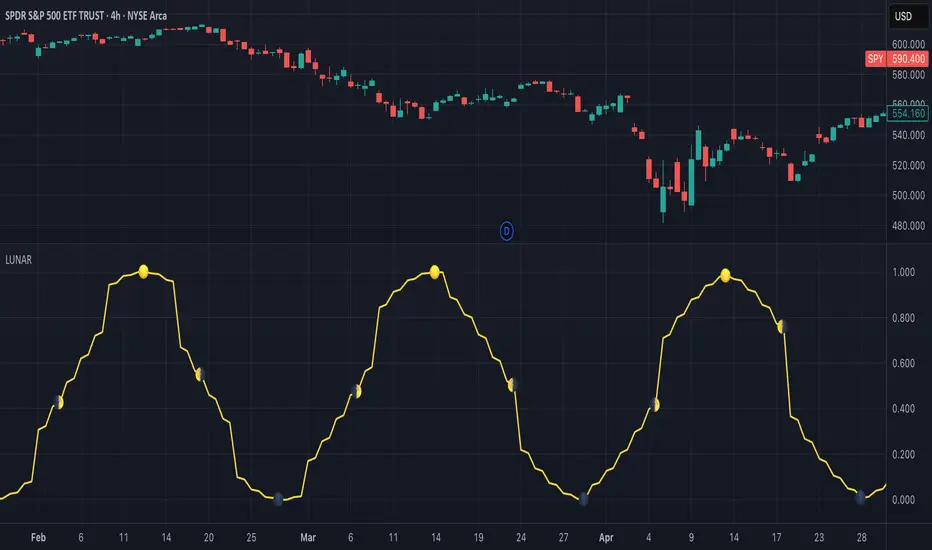
Solar Cycle (SOLAR)SOLAR: SOLAR CYCLE
🔍 OVERVIEW AND PURPOSE
The Solar Cycle indicator is an astronomical calculator that provides precise values representing the seasonal position of the Sun throughout the year. This indicator maps the Sun's position in the ecliptic to a normalized value ranging from -1.0 (winter solstice) through 0.0 (equinoxes) to +1.0 (summer solstice), creating a continuous cycle that represents the seasonal progression throughout the year.
The implementation uses high-precision astronomical formulas that include orbital elements and perturbation terms to accurately calculate the Sun's position. By converting chart timestamps to Julian dates and applying standard astronomical algorithms, this indicator achieves significantly greater accuracy than simplified seasonal approximations. This makes it valuable for traders exploring seasonal patterns, agricultural commodities trading, and natural cycle-based trading strategies.
🧩 CORE CONCEPTS
Seasonal cycle integration: Maps the annual solar cycle (365.242 days) to a continuous wave
Continuous phase representation: Provides a normalized -1.0 to +1.0 value
Astronomical precision: Uses perturbation terms and high-precision constants for accurate solar position
Key points detection: Identifies solstices (±1.0) and equinoxes (0.0) automatically
The Solar Cycle indicator differs from traditional seasonal analysis tools by incorporating precise astronomical calculations rather than using simple calendar-based approximations. This approach allows traders to identify exact seasonal turning points and transitions with high accuracy.
⚙️ COMMON SETTINGS AND PARAMETERS
Pro Tip: While the indicator itself doesn't have adjustable parameters, it's most effective when used on higher timeframes (daily or weekly charts) to visualize seasonal patterns. Consider combining it with commodity price data to analyze seasonal correlations.
🧮 CALCULATION AND MATHEMATICAL FOUNDATION
Simplified explanation:
The Solar Cycle indicator calculates the Sun's ecliptic longitude and transforms it into a sine wave that peaks at the summer solstice and troughs at the winter solstice, with equinoxes at the zero crossings.
Technical formula:
Convert chart timestamp to Julian Date:
JD = (time / 86400000.0) + 2440587.5
Calculate Time T in Julian centuries since J2000.0:
T = (JD - 2451545.0) / 36525.0
Calculate the Sun's mean longitude (L0) and mean anomaly (M), including perturbation terms:
L0 = (280.46646 + 36000.76983T + 0.0003032T²) % 360
M = (357.52911 + 35999.05029T - 0.0001537T² - 0.00000025T³) % 360
Calculate the equation of center (C):
C = (1.914602 - 0.004817T - 0.000014*T²)sin(M) +
(0.019993 - 0.000101T)sin(2M) +
0.000289sin(3M)
Calculate the Sun's true longitude and convert to seasonal value:
λ = L0 + C
seasonal = sin(λ)
🔍 Technical Note: The implementation includes terms for the equation of center to account for the Earth's elliptical orbit. This provides more accurate timing of solstices and equinoxes compared to simple harmonic approximations.
📈 INTERPRETATION DETAILS
The Solar Cycle indicator provides several analytical perspectives:
Summer Solstice (+1.0): Maximum solar elevation, longest day
Winter Solstice (-1.0): Minimum solar elevation, shortest day
Vernal Equinox (0.0 crossing up): Day and night equal length, spring begins
Autumnal Equinox (0.0 crossing down): Day and night equal length, autumn begins
Transition rates: Steepest near equinoxes, flattest near solstices
Cycle alignment: Market cycles that align with seasonal patterns may show stronger trends
Confirmation points: Solstices and equinoxes often mark important seasonal turning points
⚠️ LIMITATIONS AND CONSIDERATIONS
Geographic relevance: Solar cycle timing is most relevant for temperate latitudes
Market specificity: Seasonal effects vary significantly across different markets
Timeframe compatibility: Most effective for longer-term analysis (weekly/monthly)
Complementary tool: Should be used alongside price action and other indicators
Lead/lag effects: Market reactions to seasonal changes may precede or follow astronomical events
Statistical significance: Seasonal patterns should be verified across multiple years
Global markets: Consider opposite seasonality in Southern Hemisphere markets
📚 REFERENCES
Meeus, J. (1998). Astronomical Algorithms (2nd ed.). Willmann-Bell.
Hirshleifer, D., & Shumway, T. (2003). Good day sunshine: Stock returns and the weather. Journal of Finance, 58(3), 1009-1032.
Hong, H., & Yu, J. (2009). Gone fishin': Seasonality in trading activity and asset prices. Journal of Financial Markets, 12(4), 672-702.
Bouman, S., & Jacobsen, B. (2002). The Halloween indicator, 'Sell in May and go away': Another puzzle. American Economic Review, 92(5), 1618-1635.
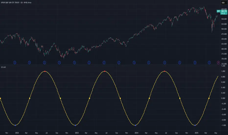
BK AK-47 Divergence🚨 Introducing BK AK-47 Divergence — Multi-Timeframe Precision Firepower for True Traders 🚨
After months of development, I’m proud to release my fifth weapon in the arsenal — BK AK-47 Divergence.
💥 Why “AK-47”? The Meaning Behind the Name
The AK-47 isn’t just a rifle. It’s the symbol of reliability, versatility, and raw stopping power. It performs in every environment — from the mud to the mountains — just like this indicator cuts through noise on any timeframe, any asset, any condition.
🔸 “AK” honors the same legacy as before — my mentor, A.K., whose discipline and vision forged my trading edge.
🔸 “47” signifies layered precision: 4 = structure, 7 = spiritual completion. Together, it’s the weapon of divine order that adapts, reacts, and strikes with purpose.
🔍 What Is BK AK-47 Divergence?
It’s a next-generation divergence detector — a smart hybrid of MACD, Bollinger Bands, and multi-timeframe divergence logic wrapped in a custom volatility engine and real-time flash alerts.
Designed for snipers in the market — those who only take the highest-probability shots.
⚙️ Core Weapon Systems
✅ MACD + BB Precision Overlay → MACD plotted inside dynamic Bollinger Bands — reveals hidden pressure zones where most indicators fail.
✅ Smart Histogram Scaling → Adaptive amplification based on volatility. No more weak histograms in strong markets.
✅ Full Multi-Timeframe Divergence Detection:
🔻 Current TF Divergence
🕐 Higher TF Divergence
⏱️ Lower TF Divergence
Each plotted with clean visual alerts, color-coded by direction and timeframe. You get instant divergence recognition across dimensions.
✅ Background Flash Alerts → When MACD hits BB extremes, the background lights up in red or green. Eyes instantly lock in on key moments.
✅ Advanced Pivot Lookback Control → New lookback system compares multiple pivot layers, not just the last swing. This gives true structural divergence, not just noise.
✅ Dynamic Fill Zones:
🔴 Oversold
🟢 Overbought
🔵 Neutral
Built to filter false signals and highlight hidden edge.
🛡️ Why This Indicator Changes the Game
🔹 Built for divergence snipers — not lagging MACD watchers.
🔹 Perfect for traders who sync with:
• Elliott Waves
• Fibonacci Time/Price Clusters
• Harmonic Patterns
• Gann Angles or Squares
• Price Action & Trendlines
🔹 Lets you visually map:
• Converging divergences (multi-TF confirmation)
• High-volatility histograms in low-volatility price zones (entry sweet spots)
• Flash-momentum warnings at BB pressure zones
🎯 How to Use BK AK-47 Divergence
🔹 Breakout Confirmation → MACD breaches upper BB with bullish divergence = signal to ride momentum.
🔹 Mean Reversion Reversals → MACD breaks lower BB + bullish div = setup for sniper long.
🔹 Top/Bottom Detection → Bearish divergence + MACD failure at upper BB = early reversal signal.
🔹 TF Sync Strategy → Align current TF with higher or lower divergences for laser-confirmed entries.
🧠 Final Thoughts
This isn’t just a divergence tool. It’s a battlefield reconnaissance system — one that lets you see when, where, and why the next pivot is forming.
🔹 Built in honor of the AK-legacy — reliability, discipline, and firepower.
🔹 Designed to cut through noise, expose structure, and alert you to what really matters.
🔹 Crafted for those who trade with intent, vision, and respect for the craft.
🙏 And most importantly: All glory to Gd — the One who gives wisdom, clarity, and purpose.
Without Him, the markets are chaos. With Him, we move in structure, order, and divine timing.
—
⚡ Stay dangerous. Stay precise. Stay aligned.
🔥 BK AK-47 Divergence — Locked. Loaded. Laser-focused. 🔥
May the markets bend to your discipline.
Gd bless. 🙏
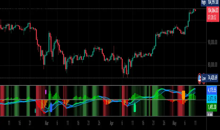
BK AK-9I am incredibly proud to introduce my fourth indicator to the TradingView community:
BK AK-9 — a next-level momentum-volatility hybrid, built for traders who demand precision.
🔥 Why “AK-9”? The Meaning Behind the Name
This indicator is deeply personal to me.
The “AK” in the name represents the initials of my mentor — the man whose guidance shaped my journey in trading, discipline, and strategy.
His wisdom is woven into every line of code, every design choice, and every purpose behind this tool.
The “9” holds its own powerful meaning:
9 is the number of completion and breakthrough — the moment where preparation meets opportunity.
The AK-9 weapon itself is a suppressed variant of the legendary AK platform, built for stealth, precision, and maximum impact in close-quarters combat.
It’s quiet, adaptive, and deadly effective — just like this indicator cuts through market noise, adapts to volatility, and pinpoints moments of maximum opportunity.
✨ About the BK AK-9 Indicator
The BK AK-9 is not just an oscillator.
It’s a multi-layered trading weapon combining:
✅ RSI → Stochastic → Bollinger Bands on Stoch RSI → momentum measured inside volatility.
✅ Dynamic or Static Background Flash → when extremes hit, you get instant visual alerts.
✅ Color-coded %K zones →
🔴 Red: oversold
🟢 Green: overbought
🔵 Blue: neutral
✅ Volatility-adaptive bands → instead of relying on static levels, the bands expand and contract dynamically using standard deviation.
🛡️ Why This Indicator Matters
Pinpoints exhaustion zones statistically, not emotionally.
Confirms breakouts with volatility evidence, not just price action.
Filters noise and helps you wait for high-probability setups.
Gives you visual edge with color-coded momentum and background flash.
Perfect for:
🔹 Breakout traders confirming momentum surges.
🔹 Mean-reversion traders catching exhaustion pivots.
🔹 Swing traders using multi-layered momentum analysis.
🔹 Momentum traders hunting volatility-backed entries.
💥 How to Use BK AK-9
Breakout Confirmation → when Stoch RSI breaks above upper Bollinger Band (green zone, flash ON), ride the trend.
Mean Reversion Trades → when Stoch RSI drops below lower Bollinger Band (red zone, flash ON), look for reversals.
Noise Filtering → stay patient inside the blue zone, wait for extremes.
Advanced Sync → align it with Gann levels, harmonic patterns, Fibonacci clusters, or Elliott waves for maximum edge.
🙏 Final Thoughts
This isn’t just another tool — it’s a weapon in your trading arsenal.
🔹 Dedicated to my mentor, A.K., whose wisdom and legacy guide my work.
🔹 Designed around the number 9, the number of completion, transition, and breakthrough.
🔹 Built to help traders act with precision, discipline, and clarity.
But above all, I give praise and glory to Gd — the true source of wisdom, insight, and success.
Markets will test your patience and your skill, but faith tests your soul. Through every challenge, every victory, and every setback, Gd remains the constant.
This tool is simply another way to use the gifts He has given — to help others rise.
⚡ Stay Ready, Stay Sharp
The markets are a battlefield. But with the right tools, the right strategy, and the right mindset — you will always stay 10 steps ahead.
🔥 Stay locked. Stay loaded. Trade with precision. 🔥
Gd bless, and may He guide us all to wisdom and success. 🙏

MA Crossover [AlchimistOfCrypto]🌌 MA Crossover Quantum – Illuminating Market Harmonic Patterns 🌌
Category: Trend Analysis Indicators 📈
"The moving average crossover, reinterpreted through quantum field principles, visualizes the underlying resonance structures of price movements. This indicator employs principles from molecular orbital theory where energy states transition through gradient fields, similar to how price momentum shifts between bullish and bearish phases. Our implementation features algorithmically optimized parameters derived from extensive Python-based backtesting, creating a visual representation of market energy flows with dynamic opacity gradients that highlight the catalytic moments where trend transformations occur."
📊 Professional Trading Application
The MA Crossover Quantum transcends the traditional moving average crossover with a sophisticated gradient illumination system that highlights the energy transfer between fast and slow moving averages. Scientifically optimized for multiple timeframes and featuring eight distinct visual themes, it enables traders to perceive trend transitions with unprecedented clarity.
⚙️ Indicator Configuration
- Timeframe Presets 📏
Python-optimized parameters for specific timeframes:
- 1H: EMA 23/395 - Ideal for intraday precision trading
- 4H: SMA 41/263 - Balanced for swing trading operations
- 1D: SMA 8/44 - Optimized for daily trend identification
- 1W: SMA 32/38 - Calibrated for medium-term position trading
- 2W: SMA 17/20 - Engineered for long-term investment signals
- Custom Settings 🎯
Full parameter customization available for professional traders:
- Fast/Slow MA Length: Fine-tune to specific market conditions
- MA Type: Select between EMA (exponential) and SMA (simple) calculation methods
- Visual Theming 🎨
Eight scientifically designed visual palettes optimized for neural pattern recognition:
- Neon (default): High-contrast green/red scheme enhancing trend transition visibility
- Cyan-Magenta: Vibrant palette for maximum visual distinction
- Yellow-Purple: Complementary colors for enhanced pattern recognition
- Specialized themes (Green-Red, Forest Green, Blue Ocean, Orange-Red, Grayscale): Each calibrated for different market environments
- Opacity Control 🔍
- Variable transparency system (0-100) allowing seamless integration with price action
- Adaptive glow effect that intensifies around crossover points - the "catalytic moments" of trend change
🚀 How to Use
1. Select Timeframe ⏰: Choose from scientifically optimized presets based on your trading horizon
2. Customize Parameters 🎚️: For advanced users, disable presets to fine-tune MA settings
3. Choose Visual Theme 🌈: Select a color scheme that enhances your personal pattern recognition
4. Adjust Opacity 🔎: Fine-tune visualization intensity to complement your chart analysis
5. Identify Trend Changes ✅: Monitor gradient intensity to spot high-probability transition zones
6. Trade with Precision 🛡️: Use gradient intensity variations to determine position sizing and risk management
Developed through rigorous mathematical modeling and extensive backtesting, MA Crossover Quantum transforms the fundamental moving average crossover into a sophisticated visual analysis tool that reveals the molecular structure of market momentum.

Relative Directional Index (RDI)🔍 Overview
The Relative Directional Index (RDI) is a hybrid tool that fuses the Average Directional and the Relative Strength Indices (ADX and RSI) into a single, highly visual interface. While the former captures trend strength, the latter reveals momentum shifts and potential exhaustion. Together, they can confirm trend structure, anticipate reversals, and sharpen the timing entries and exits.
📌 Why Combine ADX with RSI?
Most indicators focus on either trend-following (like ADX) or momentum detection (like RSI)—but rarely both. Each comes with trade-offs:
- ADX alone confirms trend strength but ignores momentum.
- RSI alone signals overbought/oversold, but lacks trend context.
The RDI resolves this by integrating both, offering:
- Smarter filters for trend entries
- Early warnings of momentum breakdowns
- More confident signal validation
🧠 Design Note: Fibonacci Harmony
All default values—5, 13, 21—are Fibonacci numbers. This is intentional, as these values reflect the natural rhythm of market cycles, and promote harmonic calibration between price action and indicator logic.
🔥 Key Features
✅ ADX Histogram
- Green bars = trend gaining strength
- Red bars = trend weakening
- Adjustable transparency for visual tuning
✅ ADX Line (Orange)
- Measures trend strength over time
- Rising = accelerating trend
- Falling = trend may be fading
✅ RSI Line (Lemon Yellow)
- Captures momentum surges and slowdowns
- Above 50 = bullish control
- Below 50 = bearish pressure
✅ Trend Strength Squares
- Bright green = strong uptrend
- Bright red = strong downtrend
- Faded colors = range-bound or indecisive
✅ ADX/RSI Crossover Markers
- Yellow square = RSI crosses above ADX → momentum building
- Orange square = ADX crosses above RSI → trend still dominant
✅ Customizable Reference Lines
- Yellow (50) = strong trend threshold
- Red (30) = weak trend zone
- Green (70) = overextended, potential exhaustion
_______________________________________________________
🎯 How to Trade with the RDI
The RDI helps traders identify momentum-supported trends, catch early reversals, and avoid false signals during consolidation.
✅ Trend Confirmation Entries
🔼 Bullish → Enter long on pullbacks or resistance breakouts
- ADX rising above 30
- RSI above 50
- Green trend square visible
🔽 Bearish → Enter short on breakdowns or failed retests
- ADX rising
- RSI below 50
- Red trend square visible
🧯 Exit if RSI crosses back against trend direction or ADX flattens
🚨 Reversal Setups Using Divergence
📈 Bullish Divergence → Long entry after confirmation (e.g. engulfing bar, volume spike)
- Price prints lower low
- RSI prints higher low
- Green triangle
📉 Bearish Divergence → Short entry on breakdown
- Price prints higher high
- RSI prints lower high
- Red triangle
Tip: Stronger if ADX is declining (fading trend strength)
🔂 Breakout Detection via Cross Markers
- Yellow square = RSI > ADX → breakout brewing
- Orange square = ADX > RSI → trend continuation likely
⏸️ Avoid Choppy Markets
- RSI between 45–55
- Faded trend squares
- Flat ADX below 20–30
🧠 Pro Tips
- Combine RDI with VWAPs, moving averages and/or pitchforks
- Watch for alignment between trend and momentum
- Use divergence markers as confirmation, not stand-alone triggers
_______________________________________________________
⚠️ Hidden Divergence (Optional)
The RDI includes optional hidden divergence detection. These signals suggest trend continuation but are off by default. Use with discretion—best in established trends, not sideways markets.
🙈 Hidden Bullish
- Price prints higher low
- RSI prints lower low
🙈 Hidden Bearish
- Price prints lower high
- RSI prints higher high

Fibonacci Time-Price Zones🟩 Fibonacci Time-Price Zones is a chart visualization tool that combines Fibonacci ratios with time-based and price-based geometry to analyze market behavior. Unlike typical Fibonacci indicators that focus solely on horizontal price levels, this indicator incorporates time into the analysis, providing a more dynamic perspective on price action.
The indicator offers multiple ways to visualize Fibonacci relationships. Drawing segmented circles creates a unique perspective on price action by incorporating time into the analysis. These segmented circles, similar to TradingView's built-in Fibonacci Circles, are derived from Fibonacci time and price levels, allowing traders to identify potential turning points based on the dynamic interaction between price and time.
As another distinct visualization method, the indicator incorporates orthogonal patterns, created by the intersection of horizontal and vertical Fibonacci levels. These intersections form L-shaped connections on the chart, derived from key Fibonacci price and time intervals, highlighting potential areas of support or resistance at specific points in time.
In addition to these geometric approaches, another option is sloped lines, which project Fibonacci levels that account for both time and price along the trendline. These projections derive their angles from the interplay between Fibonacci price levels and Fibonacci time intervals, creating dynamic zones on the chart. The slope of these lines reflects the direction and angle of the trend, providing a visual representation of price alignment with market direction, while maintaining the time-price relationship unique to this indicator
The indicator also includes horizontal Fibonacci levels similar to traditional retracement and extension tools. However, unlike standard tools, traders can display retracement levels, extension levels, or both simultaneously from a single instance of the indicator. These horizontal levels maintain consistency with the chosen visualization method, automatically scaling and adapting whether used with circles, orthogonal patterns, or slope-based analysis.
By combining these distinct methods—circles, orthogonal patterns, sloped projections, and horizontal levels—the indicator provides a comprehensive approach to Fibonacci analysis based on both time and price relationships. Each visualization method offers a unique perspective on market structure while maintaining the core principle of time-price interaction.
⭕ THEORY AND CONCEPT ⭕
While traditional Fibonacci tools excel at identifying potential support and resistance levels through price-based ratios (0.236, 0.382, 0.618), they do not incorporate the dimension of time in market analysis. Extensions and retracements effectively measure price relationships within trends, yet markets move through both price and time dimensions simultaneously.
Fibonacci circles represent an evolution in technical analysis by incorporating time intervals alongside price levels. Based on the mathematical principle that markets often move in circular patterns proportional to Fibonacci ratios, these circles project potential support and resistance zones as partial circles radiating from significant price points. However, traditional circle-based tools can create visual complexity that obscures key market relationships. The integration of time into Fibonacci analysis reveals how price movements often respect both temporal and price-based ratios, suggesting a deeper geometric structure to market behavior.
The Fibonacci Time-Price Zones indicator advances these concepts by providing multiple geometric approaches to visualize time-price relationships. Each shape option—circles, orthogonal patterns, slopes, and horizontal levels—represents a different mathematical perspective on how Fibonacci ratios manifest across both dimensions. This multi-faceted approach allows traders to observe how price responds to Fibonacci-based zones that account for both time and price movements, potentially revealing market structure that purely price-based tools might miss.
Shape Options
The indicator employs four distinct geometric approaches to analyze Fibonacci relationships across time and price dimensions:
Circular : Represents the cyclical nature of market movements through partial circles, where each radius is scaled by Fibonacci ratios incorporating both time and price components. This geometry suggests market movements may follow proportional circular paths from significant pivot points, reflecting the harmonic relationship between time and price.
Orthogonal : Constructs L-shaped patterns that separate the time and price components of Fibonacci relationships. The horizontal component represents price levels, while the vertical component measures time intervals, allowing analysis of how these dimensions interact independently at key market points.
Sloped : Projects Fibonacci levels along the prevailing trend, incorporating both time and price in the angle of projection. This approach suggests that support and resistance levels may maintain their relationship to price while adjusting to the temporal flow of the market.
Horizontal : Provides traditional static Fibonacci levels that serve as a reference point for comparing price-only analysis with the dynamic time-price relationships shown in the other three shapes. This baseline approach allows traders to evaluate how the incorporation of time dimension enhances or modifies traditional Fibonacci analysis.
By combining these geometric approaches, the Fibonacci Time-Price Zones indicator creates a comprehensive analytical framework that bridges traditional and advanced Fibonacci analysis. The horizontal levels serve as familiar reference points, while the dynamic elements—circular, orthogonal, and sloped projections—reveal how price action responds to temporal relationships. This multi-dimensional approach enables traders to study market structure through various geometric lenses, providing deeper insights into time-price symmetry within technical analysis. Whether applied to retracements, extensions, or trend analysis, the indicator offers a structured methodology for understanding how markets move through both price and time dimensions.
🛠️ CONFIGURATION AND SETTINGS 🛠️
The Fibonacci Time-Price Zones indicator offers a range of configurable settings to tailor its functionality and visual representation to your specific analysis needs. These options allow you to customize zone visibility, structures, horizontal lines, and other features.
Important Note: The indicator's calculations are anchored to user-defined start and end points on the chart. When switching between charts with significantly different price scales (e.g., from Bitcoin at $100,000 to Silver at $30), adjustment of these anchor points is required to ensure correct positioning of the Fibonacci elements.
Fibonacci Levels
The indicator allows users to customize Fibonacci levels for both retracement and extension analysis. Each level can be individually configured with the following options:
Visibility : Toggle the visibility of each level to focus on specific areas of interest.
Level Value : Set the Fibonacci ratio for the level, such as 0.618 or 1.000, to align with your analysis needs.
Color : Customize the color of each level for better visual clarity.
Line Thickness : Adjust the line thickness to emphasize critical levels or maintain a cleaner chart.
Setup
Zone Type : Select which Fibonacci zones to display:
- Retracement : Shows potential pull back levels within the trend
- Extension : Projects levels beyond the trend for potential continuation targets
- Both : Displays both retracement and extension zones simultaneously
Shape : Choose from four visualization methods:
- Circular : Time-price based semicircles centered on point B
- Orthogonal : L-shaped patterns combining time and price levels
- Sloped : Trend-aligned projections of Fibonacci levels
- Horizontal : Traditional horizontal Fibonacci levels
Visual Settings
Fill % : Adjusts the fill intensity of zones:
0% : No fill between levels
100% : Maximum fill between levels
Lines :
Trendline : The base A-B trend with customizable color
Extension : B-C projection line
Retracement : B-D pullback line
Labels :
Points : Show/hide A, B, C, D markers
Levels : Show/hide Fibonacci percentages
Time-Price Points
Set the time and price for the points that define the Fibonacci zones and horizontal levels. These points are defined upon loading the chart. These points can be configured directly in the settings or adjusted interactively on the live chart.
A and B Points : These user-defined time and price points determine the basis for calculating the semicircles and Fibonacci levels. While the settings panel displays their exact values for fine-tuning, the easiest way to modify these points is by dragging them directly on the chart for quick adjustments.
Interactive Adjustments : Any changes made to the points on the chart will automatically synchronize with the settings panel, ensuring consistency and precision.
🖼️ CHART EXAMPLES 🖼️
Fibonacci Time-Price Zones using the 'Circular' Shape option. Note the price interaction at the 0.786 level, which acts as a support zone. Additional points of interest include resistance near the 0.618 level and consolidation around the 0.5 level, highlighting the utility of both horizontal and semicircular Fibonacci projections in identifying key price areas.
Fibonacci Time-Price Zones using the 'Sloped' Shape option. The chart displays price retracing along the sloped Fibonacci levels, with blue arrows highlighting potential support zones at 0.618 and 0.786, and a red arrow indicating potential resistance at the 1.0 level. This visual representation aligns with the prevailing downtrend, suggesting potential selling pressure at the 1.0 Fibonacci level.
Fibonacci Time-Price Zones using the 'Orthogonal' Shape option. The chart demonstrates price action interacting with vertical zones created by the orthogonal lines at the 0.618, 0.786, and 1.0 Fibonacci levels. Blue arrows highlight potential support areas, while red arrows indicate potential resistance areas, revealing how the orthogonal lines can identify distinct points of price interaction.
Fibonacci Time-Price Zones using the 'Circular' Shape option. The chart displays price action in relation to segmented circles emanating from the starting point (point A). The circles represent different Fibonacci ratios (0.382, 0.5, 0.618, 0.786) and their intersections with the price axis create potential zones of support and resistance. This approach offers a visually distinct way to analyze potential turning points based on both price and time.
Fibonacci Time-Price Zones using the 'Sloped' Shape option. The sloped Fibonacci levels (0.786, 0.618, 0.5) create zones of potential support and resistance, with price finding clear interaction within these areas. The ellipses highlight this price action, particularly the support between 0.786 and 0.618, which aligns closely with the trend.
Fibonacci Time-Price Zones using the 'Circular' Shape option. The price action appears to be ‘hugging’ the 0.5 Fibonacci level, suggesting potential resistance. This demonstrates how the circular zones can identify potential turning points and areas of consolidation which might not be seen with linear analysis.
Fibonacci Time-Price Zones using the 'Sloped' Shape option with Point D marker enabled. The chart demonstrates clear price action closely following along the sloped Retracement line until the orthogonal intersection at the 0.618 levels where the trend is broken and price dips throughout the 0.618 to 0.786 horizontal zone. Price jumps back to the retracement slope at the start of the 0.786 horizontal zone and continues to the 1.0 horizontal zone. The aqua-colored retracement line is enabled to further emphasize this retracement slope .
Geometric validation using TradingView's built-in Fibonacci Circle tool (overlaid). The alignment at the 0.5 and 1.0 levels demonstrates the indicator's consistent approximation of Fibonacci Circles.
Comparison of Fibonacci Time-Price Zones (Shape: Horizontal) with TradingView's Built-in Retracement and Extension Tools (overlaid): This example demonstrates how the Horizontal structure aligns with TradingView’s retracement and extension levels, allowing users to integrate multiple tools seamlessly. The Fibonacci circle connects retracement and extension zones, highlighting the potential relationship between past retracements and future extensions.
📐 GEOMETRIC FOUNDATIONS 📐
This indicator integrates circular and straight representations of Fibonacci levels, specifically the Circular , Orthogonal , Sloped , and Horizontal shape options. The geometric principles behind these shapes differ significantly, requiring distinct scaling methods for accurate representation. The Circular shape employs logarithmic scaling with radial expansion, where the distance from a central point determines the level's position, creating partial circles that align with TradingView's built-in Fibonacci Circle tool. The other three shapes utilize geometric progression scaling for linear extension from a starting point, resulting in straight lines that align with TradingView's built-in Fibonacci retracement and extension tools. Due to these distinct geometric foundations and scaling methods, perfectly aligning both the partial circles and straight lines simultaneously is mathematically constrained, though any differences are typically visually imperceptible.
The Circular shape's partial circles are calculated and scaled to align with TradingView's built-in Fibonacci Circles. These circles are plotted from the second swing point onward. This approach ensures consistent and accurate visualization across all market types, including those with gaps or closed sessions, which unlike 24/7 markets, do not have a direct one-to-one correspondence between bar indices and time. To maintain accurate geometric proportions across varying chart scales, the indicator calculates an aspect ratio by normalizing the proportional difference between vertical (price) and horizontal (time) distances of the swing points. This normalization factor ensures geometric shapes maintain their mathematical properties regardless of price scale magnitude or time period span, while maintaining the correct proportions of the geometric constructions at any chart zoom level.
The indicator automatically applies the appropriate scaling factor based on the selected shape option, optimizing either circular proportions and proper radius calculations for each Fibonacci level, or straight-line relationships between Fibonacci levels. These distinct scaling approaches maintain mathematical integrity while preserving the essential characteristics of each geometric representation, ensuring optimal visualization accuracy whether using circular or linear shapes.
⚠️ DISCLAIMER ⚠️
The Fibonacci Time-Price Zones indicator is a visual analysis tool designed to illustrate Fibonacci relationships through geometric constructions incorporating both curved and straight lines, providing a structured framework for identifying potential areas of price interaction. It is not intended as a predictive or standalone trading signal indicator.
The indicator calculates levels and projections using user-defined anchor points and Fibonacci ratios. While it aims to align with TradingView’s Fibonacci extension, retracement, and circle tools by employing mathematical and geometric formulas, no guarantee is made that its calculations are identical to TradingView's proprietary methods.
Like all technical and visual indicators, these visual representations may visually align with key price zones in hindsight, reflecting observed price dynamics. However, these visualizations are not standalone signals for trading decisions and should be interpreted as part of a broader analytical approach.
This indicator is intended for educational and analytical purposes, complementing other tools and methods of market analysis. Users are encouraged to integrate it into a comprehensive trading strategy, customizing its settings to suit their specific needs and market conditions.
🧠 BEYOND THE CODE 🧠
The Fibonacci Time-Price Zones indicator is designed to encourage both education and community engagement. By integrating time-sensitive geometry with Fibonacci-based frameworks, it bridges traditional grid-based analysis with dynamic time-price relationships. The inclusion of semicircles, horizontal levels, orthogonal structures, and sloped trends provides users with versatile tools to explore the interaction between price movements and temporal intervals while maintaining clarity and adaptability.
As an open-source tool, the indicator invites exploration, experimentation, and customization. Whether used as a standalone resource or alongside other technical strategies, it serves as a practical and educational framework for understanding market structure and Fibonacci relationships in greater depth.
Your feedback and contributions are essential to refining and enhancing the Fibonacci Time-Price Zones indicator. We look forward to the creative applications, adaptations, and insights this tool inspires within the trading community.

N-Degree Moment-Based Adaptive Detection🙏🏻 N-Degree Moment-Based Adaptive Detection (NDMBAD) method is a generalization of MBAD since the horizontal line fit passing through the data's mean can be simply treated as zero-degree polynomial regression. We can extend the MBAD logic to higher-degree polynomial regression.
I don't think I need to talk a lot about the thing there; the logic is really the same as in MBAD, just hit the link above and read if you want. The only difference is now we can gather cumulants not only from the horizontal mean fit (degree = 0) but also from higher-order polynomial regression fit, including linear regression (degree = 1).
Why?
Simply because residuals from the 0-degree model don't contain trend information, and while in some cases that's exactly what you need, in other cases, you want to model your trend explicitly. Imagine your underlying process trends in a steady manner, and you want to control the extreme deviations from the process's core. If you're going to use 0-degree, you'll be treating this beautiful steady trend as a residual itself, which "constantly deviates from the process mean." It doesn't make much sense.
How?
First, if you set the length to 0, you will end up with the function incrementally applied to all your data starting from bar_index 0. This can be called the expanding window mode. That's the functionality I include in all my scripts lately (where it makes sense). As I said in the MBAD description, choosing length is a matter of doing business & applied use of my work, but I think I'm open to talk about it.
I don't see much sense in using degree > 1 though (still in research on it). If you have dem curves, you can use Fourier transform -> spectral filtering / harmonic regression (regression with Fourier terms). The job of a degree > 0 is to model the direction in data, and degree 1 gets it done. In mean reversion strategies, it means that you don't wanna put 0-degree polynomial regression (i.e., the mean) on non-stationary trending data in moving window mode because, this way, your residuals will be contaminated with the trend component.
By the way, you can send thanks to @aaron294c , he said like mane MBAD is dope, and it's gonna really complement his work, so I decided to drop NDMBAD now, gonna be more useful since it covers more types of data.
I wanned to call it N-Order Moment Adaptive Detection because it abbreviates to NOMAD, which sounds cool and suits me well, because when I perform as a fire dancer, nomad style is one of my outfits. Burning Man stuff vibe, you know. But the problem is degree and order really mean two different things in the polynomial context, so gotta stay right & precise—that's the priority.
∞

Bitcoin Wave RainbowThis Bitcoin Wave Rainbow model is a powerful tool designed to help traders of all levels understand and navigate the Bitcoin market. It works only with BTC in any timeframe, but better looks in dayly or weekly timeframes. It provides valuable insights into historical price behavior and offers forecasts for the next decade, making it an essential asset for both short-term and long-term strategies.
How the Model Works
The model is built on a logarithmic trend, also known as a power law, represented by the green line on the chart. This line illustrates the expected price trajectory of Bitcoin over time. The model also incorporates a range of price fluctuations around this trend, represented by colored bands.
The width of these bands narrows over time, indicating that the model becomes increasingly accurate as it progresses. This is due to the exponential decrease in the range of price fluctuations, making the model a reliable tool for predicting future price movements.
Understanding the Zones
Blue Zone: This zone signifies that the price is below its trend, making it a recommended area for buying Bitcoin. It represents a level where the price is unlikely to fall further, providing a potential opportunity for accumulation.
Green Zone: This zone represents a fair price range, where the price is relatively close to its trend. In this zone, the price may continue to go up or down, depending on the halving season. ransiting up around any halving and transiting down around 2 years after each halving.
Yellow Zone: This zone indicates that the price is somewhat overheated, often due to the hype following a halving event. While there may still be room for the price to rise, traders should exercise caution in this zone, as a price correction could occur.
Red Zone: This zone represents a strong overbought condition, where the price is significantly above its trend. Traders should be extremely cautious in this zone and consider reducing their positions, as the price is likely to revert back towards the trend or even lower.
Using the Model in Your Trading Strategy
This indicator can be used in conjunction with the Bitcoin Wave Model, which complements it by showing harmonic price fluctuations associated with halving events. Together, these indicators provide a comprehensive view of the Bitcoin market, allowing traders to make informed decisions based on both historical data and future projections.
Benefits for Traders
This Bitcoin price model offers numerous benefits for traders, including:
Clear Visualization: The model provides a clear and concise visual representation of Bitcoin's price behavior, making it easy to understand and interpret.
Accurate Forecasting: The model's accuracy increases over time, providing reliable forecasts for future price movements.
Risk Management: The model helps traders identify overbought and oversold conditions, allowing them to manage their risk more effectively.
Strategic Decision-Making: By understanding the different zones and their implications, traders can make more informed decisions about when to buy, sell, or hold Bitcoin.
By incorporating this Bitcoin price model into your trading strategy, you can gain a deeper understanding of the market dynamics and improve your chances of success.

[AIO] Multi Collection Moving Averages 140 MA TypesAll In One Multi Collection Moving Averages.
Since signing up 2 years ago, I have been collecting various Сollections.
I decided to get it into a decent shape and make it one of the biggest collections on TV, and maybe the entire internet.
And now I'm sharing my collection with you.
140 Different Types of Moving Averages are waiting for you.
Specifically :
"
AARMA | Adaptive Autonomous Recursive Moving Average
ADMA | Adjusted Moving Average
ADXMA | Average Directional Moving Average
ADXVMA | Average Directional Volatility Moving Average
AHMA | Ahrens Moving Average
ALF | Ehler Adaptive Laguerre Filter
ALMA | Arnaud Legoux Moving Average
ALSMA | Adaptive Least Squares
ALXMA | Alexander Moving Average
AMA | Adaptive Moving Average
ARI | Unknown
ARSI | Adaptive RSI Moving Average
AUF | Auto Filter
AUTL | Auto-Line
BAMA | Bryant Adaptive Moving Average
BFMA | Blackman Filter Moving Average
CMA | Corrected Moving Average
CORMA | Correlation Moving Average
COVEMA | Coefficient of Variation Weighted Exponential Moving Average
COVNA | Coefficient of Variation Weighted Moving Average
CTI | Coral Trend Indicator
DEC | Ehlers Simple Decycler
DEMA | Double EMA Moving Average
DEVS | Ehlers - Deviation Scaled Moving Average
DONEMA | Donchian Extremum Moving Average
DONMA | Donchian Moving Average
DSEMA | Double Smoothed Exponential Moving Average
DSWF | Damped Sine Wave Weighted Filter
DWMA | Double Weighted Moving Average
E2PBF | Ehlers 2-Pole Butterworth Filter
E2SSF | Ehlers 2-Pole Super Smoother Filter
E3PBF | Ehlers 3-Pole Butterworth Filter
E3SSF | Ehlers 3-Pole Super Smoother Filter
EDMA | Exponentially Deviating Moving Average (MZ EDMA)
EDSMA | Ehlers Dynamic Smoothed Moving Average
EEO | Ehlers Modified Elliptic Filter Optimum
EFRAMA | Ehlers Modified Fractal Adaptive Moving Average
EHMA | Exponential Hull Moving Average
EIT | Ehlers Instantaneous Trendline
ELF | Ehler Laguerre filter
EMA | Exponential Moving Average
EMARSI | EMARSI
EPF | Edge Preserving Filter
EPMA | End Point Moving Average
EREA | Ehlers Reverse Exponential Moving Average
ESSF | Ehlers Super Smoother Filter 2-pole
ETMA | Exponential Triangular Moving Average
EVMA | Elastic Volume Weighted Moving Average
FAMA | Following Adaptive Moving Average
FEMA | Fast Exponential Moving Average
FIBWMA | Fibonacci Weighted Moving Average
FLSMA | Fisher Least Squares Moving Average
FRAMA | Ehlers - Fractal Adaptive Moving Average
FX | Fibonacci X Level
GAUS | Ehlers - Gaussian Filter
GHL | Gann High Low
GMA | Gaussian Moving Average
GMMA | Geometric Mean Moving Average
HCF | Hybrid Convolution Filter
HEMA | Holt Exponential Moving Average
HKAMA | Hilbert based Kaufman Adaptive Moving Average
HMA | Harmonic Moving Average
HSMA | Hirashima Sugita Moving Average
HULL | Hull Moving Average
HULLT | Hull Triple Moving Average
HWMA | Henderson Weighted Moving Average
IE2 | Early T3 by Tim Tilson
IIRF | Infinite Impulse Response Filter
ILRS | Integral of Linear Regression Slope
JMA | Jurik Moving Average
KA | Unknown
KAMA | Kaufman Adaptive Moving Average & Apirine Adaptive MA
KIJUN | KIJUN
KIJUN2 | Kijun v2
LAG | Ehlers - Laguerre Filter
LCLSMA | 1LC-LSMA (1 line code lsma with 3 functions)
LEMA | Leader Exponential Moving Average
LLMA | Low-Lag Moving Average
LMA | Leo Moving Average
LP | Unknown
LRL | Linear Regression Line
LSMA | Least Squares Moving Average / Linear Regression Curve
LTB | Unknown
LWMA | Linear Weighted Moving Average
MAMA | MAMA - MESA Adaptive Moving Average
MAVW | Mavilim Weighted Moving Average
MCGD | McGinley Dynamic Moving Average
MF | Modular Filter
MID | Median Moving Average / Percentile Nearest Rank
MNMA | McNicholl Moving Average
MTMA | Unknown
MVSMA | Minimum Variance SMA
NLMA | Non-lag Moving Average
NWMA | Dürschner 3rd Generation Moving Average (New WMA)
PKF | Parametric Kalman Filter
PWMA | Parabolic Weighted Moving Average
QEMA | Quadruple Exponential Moving Average
QMA | Quick Moving Average
REMA | Regularized Exponential Moving Average
REPMA | Repulsion Moving Average
RGEMA | Range Exponential Moving Average
RMA | Welles Wilders Smoothing Moving Average
RMF | Recursive Median Filter
RMTA | Recursive Moving Trend Average
RSMA | Relative Strength Moving Average - based on RSI
RSRMA | Right Sided Ricker MA
RWMA | Regressively Weighted Moving Average
SAMA | Slope Adaptive Moving Average
SFMA | Smoother Filter Moving Average
SMA | Simple Moving Average
SSB | Senkou Span B
SSF | Ehlers - Super Smoother Filter P2
SSMA | Super Smooth Moving Average
STMA | Unknown
SWMA | Self-Weighted Moving Average
SW_MA | Sine-Weighted Moving Average
TEMA | Triple Exponential Moving Average
THMA | Triple Exponential Hull Moving Average
TL | Unknown
TMA | Triangular Moving Average
TPBF | Three-pole Ehlers Butterworth
TRAMA | Trend Regularity Adaptive Moving Average
TSF | True Strength Force
TT3 | Tilson (3rd Degree) Moving Average
VAMA | Volatility Adjusted Moving Average
VAMAF | Volume Adjusted Moving Average Function
VAR | Vector Autoregression Moving Average
VBMA | Variable Moving Average
VHMA | Vertical Horizontal Moving Average
VIDYA | Variable Index Dynamic Average
VMA | Volume Moving Average
VSO | Unknown
VWMA | Volume Weighted Moving Average
WCD | Unknown
WMA | Weighted Moving Average
XEMA | Optimized Exponential Moving Average
ZEMA | Zero Lag Moving Average
ZLDEMA | Zero-Lag Double Exponential Moving Average
ZLEMA | Ehlers - Zero Lag Exponential Moving Average
ZLTEMA | Zero-Lag Triple Exponential Moving Average
ZSMA | Zero-Lag Simple Moving Average
"
Don't forget that you can use any Moving Average not only for the chart but also for any of your indicators without affecting the code as in my example.
But remember that some MAs are not designed to work with anything other than a chart.
All MA and Code lists are sorted strictly alphabetically by short name (A-Z).
Each MA has its own number (ID) by which you can display the Moving Average you need.
Next to the ID selection there are tooltips with short names and their numbers. Use them.
The panel below will help you to read the Name of the selected MA.
Because of the size of the collection I think this is the optimal and most convenient use. Correct me if this is not the case.
Unknown - Some MAs I collected so long ago that I lost the full real name and couldn't find the authors. If you recognize them, please let me know.
I have deliberately simplified all MAs to input just Source and Length.
Because the collection is so large, it would be quite inconvenient and difficult to customize all MA functions (multipliers, offset, etc.).
If you need or like any MA you will still have to take it from my collection for your code.
I tried to leave the basic MA settings inside function in first strings.
I have tried to list most of the authors, but since the bulk of the collection was created a long time ago and was not intended for public publication I could not find all of them.
Some of the features were created from scratch or may have been slightly modified, so please be careful.
If you would like to improve this collection, please write to me in PM.
Also Credits, Likes, Awards, Loves and Thanks to :
@alexgrover
@allanster
@andre_007
@auroagwei
@blackcat1402
@bsharpe
@cheatcountry
@CrackingCryptocurrency
@Duyck
@ErwinBeckers
@everget
@glaz
@gotbeatz26107
@HPotter
@io72signals
@JacobAmos
@JoshuaMcGowan
@KivancOzbilgic
@LazyBear
@loxx
@LuxAlgo
@MightyZinger
@nemozny
@NGBaltic
@peacefulLizard50262
@RicardoSantos
@StalexBot
@ThiagoSchmitz
@TradingView
— 𝐀𝐧𝐝 𝐎𝐭𝐡𝐞𝐫𝐬 !
So just a Big Thank You to everyone who has ever and anywhere shared their codes.
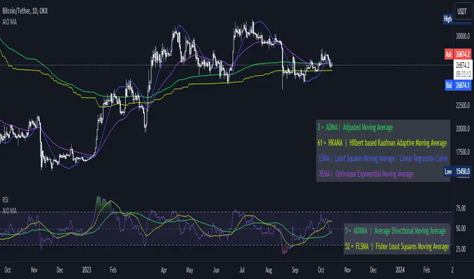
Dominant Period-Based Moving Average (DPBMA)Exploit Market Cycles with the Dominant Period-Based Moving Average Indicator
Introduction:
In the world of trading, market cycles play a crucial role in determining the rhythm of the market. These cycles often consist of recurring patterns that traders can exploit to maximize their profits. One effective way to capitalize on these cycles is by using a moving average (MA) indicator. Today, we are going to introduce you to a unique indicator that takes the most frequent dominant period of the market and uses it as the length of the moving average. This indicator is designed to adapt to the ever-changing market conditions, providing traders with a dynamic tool to better analyze the market.
Dominant Period-Based Moving Average Indicator Overview:
The Dominant Period-Based Moving Average (DPBMA) Indicator is a custom indicator designed to find the most frequent dominant period of the market and use that period as the length of the moving average. This innovative approach allows the indicator to adapt to the market cycles, making it more responsive to the market's changing conditions.
Here's a quick overview of the DPBMA Indicator's features:
Takes the most frequent dominant period of the market.
Uses the dominant period as the length of the moving average.
Adapts to the changing market cycles.
Works as an overlay on your price chart.
Using the Dominant Period-Based Moving Average Indicator:
How the Dominant Period-Based Moving Average Indicator Works:
The DPBMA Indicator works by first importing the DominantCycle function from the lastguru/DominantCycle/2 script. This function calculates the dominant cycle period of the given market data. The DPBMA Indicator then calculates the Exponential Moving Average (EMA) using the dominant period as the length parameter.
The EMA calculation uses an alpha factor, which is calculated as 2 / (length + 1). The alpha factor is then used to smooth the source data (closing prices) and calculate the adaptive moving average.
The DPBMA Indicator also includes a harmonic input, which allows you to multiply the dominant cycle period by an integer value. This can help you fine-tune the indicator to better fit your trading strategy or style.
The Raw Dominant Frequency:
The raw dominant frequency represents the primary cycle period present in the given market data. By identifying the raw dominant frequency, traders can gain insights into the market's current cycle and use this information to make informed trading decisions. The raw dominant frequency can be useful for detecting major trend reversals, support and resistance levels, and potential entry and exit points.
However, using the raw dominant frequency alone has its limitations. For instance, it may not always provide a clear picture of the market's prevailing trend, especially during periods of high market volatility. Additionally, relying solely on the raw dominant frequency may not capture the nuances of shorter-term cycles that can also impact price movements.
The Most Likely Dominant Frequency:
Our approach takes a different angle by focusing on the most likely dominant frequency. This method aims to identify the frequency with the highest probability of being the dominant frequency in the market data. The idea behind this approach is to filter out potential noise and improve the accuracy of the dominant frequency analysis. By using the most likely dominant frequency, traders can gain a more reliable understanding of the market's primary cycle, which can lead to better trading decisions.
In our Dominant Period-Based Moving Average Indicator, we calculate the most likely dominant frequency by analyzing an array of cycle periods and their occurrences in the given market data. We then determine the cycle period with the highest occurrence, representing the most likely dominant frequency. This method allows the indicator to be more adaptive and responsive to the changing market conditions, capturing the nuances of both long-term and short-term cycles.
Why Not the Average Dominant Frequency?
While using the average dominant frequency might seem like a reasonable approach, it can be less effective in accurately capturing the market's primary cycle. Averaging the dominant frequencies may dilute the impact of the true dominant frequency, resulting in a less accurate representation of the market's current cycle. By focusing on the most likely dominant frequency, our approach provides a more accurate and reliable analysis of the market's primary cycle, which can ultimately lead to more effective trading decisions.
Conclusion:
The Dominant Period-Based Moving Average Indicator, enhanced with the most likely dominant frequency approach, offers traders a powerful tool for exploiting market cycles. By adapting to the most frequent dominant period and focusing on the most likely dominant frequency, this indicator provides a more accurate and reliable analysis of the market's primary cycle. As a result, traders can make better-informed decisions, ultimately leading to improved trading performance. Incorporate the DPBMA Indicator into your trading toolbox today, and take advantage of the enhanced market analysis it provides.
Automated Option Price - Black-Scholes modelPlease make sure you are plotting this indicator on DAILY bars, not doing so will lead to unintended results. Also, make sure that you keep up to date the Risk-free interest rate, which you can consult (for U.S.) on ycharts.com.
This is an indicator that is meant to be used for Options Day Trading, but it can be useful for mid-term or leaps for I also enabled the possibility for user to input manually the Strike and Expiration date. I based the calculation on the Black-Scholes model. Variables included in the calculation are:
-Stock price (S): The current price of the underlying asset (e.g., a stock).
-Strike price (K): The predetermined price at which the option can be exercised.
-Time to expiration (T): The time remaining until the option expires, expressed as a fraction of a year.
-Volatility (σ): The annualized standard deviation of the stock's returns, which is a measure of the stock's price fluctuations.
-Risk-free interest rate (r): The annualized return on a risk-free investment, often approximated by the yield on a government bond.
The only variable I excluded from the original model was the Dividend yield (q).
U S E R I N P U T S:
1. AUTOMATIC calculations enabled:
i) Strike price (K):
Automatically calculate the strike price for both call and put options based on the stock's closing price. The logic follows a set of rules to determine the strike prices which will usually be Out-of-the-Money (OTM):
-If the stock's closing price is between 1 and 60, the call strike price is rounded up to the nearest whole number, while the put strike price is rounded down to the nearest whole number.
-If the stock's closing price is between 60 and 90, the call strike price is rounded up to the nearest whole number and increased by 1, while the put strike price is rounded down to the nearest whole number and decreased by 1.
-If the stock's closing price is between 90 and 120, the call strike price is rounded up to the nearest whole number and increased by 2, while the put strike price is rounded down to the nearest whole number and decreased by 2.
-If the stock's closing price is above 120, the call strike price is rounded up to the nearest multiple of 5, while the put strike price is rounded down to the nearest multiple of 5.
By applying these rules, I just tried to ensure that the automatically calculated strike prices are tailored to the stock's price range, allowing for more accurate option pricing calculations.
ii) Time to expiration (T):
The indicator will consider this week’s expiration contracts (Friday) only when the current day/bar = Monday. If Tuesday or older it will consider the expiration date of the next week’s Friday (because we are not Theta gamblers, right?).
If you are not comfortable with above for whatever reason, you can always…
2. Enter inputs MANUALLY
First make sure you UNTICK the boxes for automatic calculation.
i) Strike price (K) – Self-explanatory
ii) Time to expiration (T) – Just make sure that the horizon you are inputting matches with the next parameter (e.g. you would not input a Monthly risk-free interest rate for a Leap).
iii) Risk-free interest rate (r) – You can pull this data from the web. Here’s the link I used to define the value that this indicator was launched with:
ycharts.com
Don’t get obsessed with updating this daily if you are using this for day trading, you will notice that weekly may be more than enough.
V O L A T I L I T Y
Not option to manually input Volatility so I’ll explain how it is calculated in this script:
I considered two measures of volatility; one is derived calculating the annualized volatility using the standard deviation of daily returns and the second one is the ATR-based annualized volatility. I then used a ‘combined’ approach with the harmonic mean and the arithmetic mean of these results which can help account for the variability in the option prices calculated with different volatility estimates, which can be more robust when dealing with outliers or skewed data. I back tested with some samples of actual option prices and found that this approach is the one that got results closer to the actual bids.
T A B L E
Nomenclature to read rows is:
Option Strike Price | Type of Option (Put or Call) @ The current Close or at 50% level of bar | Estimated Price
*The Option expiration Date showed as dd-MMM as part of the headers.
Second and third row (color 1): These will show the calculated value for the Put/Call, assuming you are buying at the CURRENT price of the stock.
Third and Fifth row (color2): These will show the calculated value for the Put/Call, assuming you buy at the 50% level of the current bar (this is the value that the contract WOULD HAVE at the 50% level of the bar).
If you plot the indicator during market hours it will obviously update as price moves, this is an intended feature.
L I M I T A T I O N S
The Black-Scholes model, like many other models, has its limitations and will oftentimes provide inaccurate option prices in all market conditions. High volatility events, such as earnings announcements, can lead to significant price fluctuations that are not fully captured by the model.
The model assumes that the stock price follows a continuous random walk with constant volatility, but in reality, volatility can change over time, and stock prices can exhibit jumps, especially around significant events like earnings announcements. This can cause the model to underestimate the true option price in such situations.
Please make sure that you first back test on the symbols you trade to ensure the information presented by this indicator will suit your trading strategy. You will find that the delta between the proposed price of the indicator versus the actual price may differ significantly in some symbols while for others it will be very close. For instance, today (13APR23), the prices for AMD, DIS, AAPL (puts only), were very close to actual bids, whereas TSLA differ significantly (but then again, take a look at the calendar and this last symbol is having earnings next week which may add a premium to the contracts)… I am sure you will get your own conclusions and applicable use cases based on the data you test with.
As always, be wise and methodical on the investment or trading decisions you make!
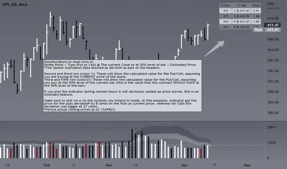
Dominant Cycle Detection OscillatorThis is a Dominant Cycle Detection Oscillator that searches multiple ranges of wavelengths within a spectrum. Choose one of 4 different dominant cycle detection methods (MESA MAMA cycle, Pearson Autocorrelation, Discreet Fourier Transform, and Phase Accumulation) to determine the most dominant cycles and see the historical results. Straight lines can indicate a steady dominant cycle; while Wavy lines might indicate a varying dominant cycle length. The steadier the cycle, the easier it may be to predict future events in that cycle (keep the log scale in mind when considering steadiness). The presence of evenly divisible (or harmonic) cycle lengths may also indicate stronger cycles; for example, 19, 38, and 76 dominant lengths for the 2x, 4x, and 8x cycles. Practically, a trader can use these cycle outputs as the default settings for other Hurst/cycle indicators. For example, if you see dominant cycle oscillator outputs of 38 & 76 for the 4x and 8x cycle respectively, you might want to test/use defaults of 38 & 76 for the 4x & 8x lengths in the bandpass, diamond/semi-circle notation, moving average & envelope, and FLD instead of the defaults 40 & 80 for a more fine-tuned analysis.
Muting the oscillator's historical lines and overlaying the indicator on the chart can visually cue a trader to the cycle lengths without taking up extra panes. The DFT Cycle lengths with muted historical lines have been overlayed on the chart in the photo.
The y-axis scale for this indicator's pane (just the oscillator pane, not the chart) most likely needs to be changed to logarithmic to look normal, but it depends on the search ranges in your settings. There are instructions in the settings. In the photo, the MESA MAMA scale is set to regular (not logarithmic) which demonstrates how difficult it can be to read if not changed.
In the Spectral Analysis chapter of Hurst's book Profit Magic, he recommended doing a Fourier analysis across a spectrum of frequencies. Hurst acknowledged there were many ways to do this analysis but recommended the method described by Lanczos. Currently in this indicator, the closest thing to the method described by Lanczos is the DFT Discreet Fourier Transform method.
Shoutout to @lastguru for the dominant cycle library referenced in this code. He mentioned that he may add more methods in the future.
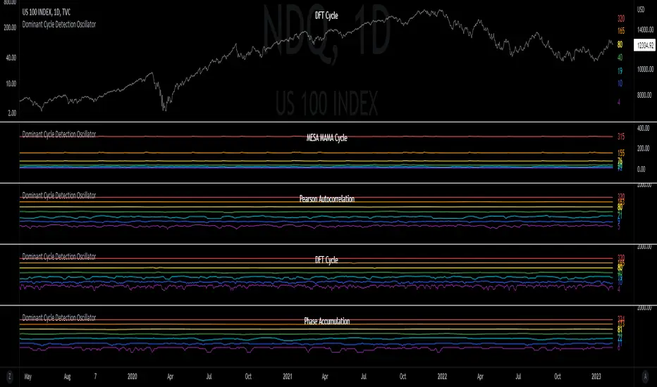
Channel Based Zigzag [HeWhoMustNotBeNamed]🎲 Concept
Zigzag is built based on the price and number of offset bars. But, in this experiment, we build zigzag based on different bands such as Bollinger Band, Keltner Channel and Donchian Channel. The process is simple:
🎯 Derive bands based on input parameters
🎯 High of a bar is considered as pivot high only if the high price is above or equal to upper band.
🎯 Similarly low of a bar is considered as pivot low only if low price is below or equal to lower band.
🎯 Adding the pivot high/low follows same logic as that of regular zigzag where pivot high is always followed by pivot low and vice versa.
🎯 If the new pivot added is of same direction as that of last pivot, then both pivots are compared with each other and only the extreme one is kept. (Highest in case of pivot high and lowest in case of pivot low)
🎯 If a bar has both pivot high and pivot low - pivot with same direction as previous pivot is added to the list first before adding the pivot with opposite direction.
🎲 Use Cases
Can be used for pattern recognition algorithms instead of standard zigzag. This will help derive patterns which are relative to bands and channels.
Example: John Bollinger explains how to manually scan double tap using Bollinger Bands in this video: www.youtube.com This modified zigzag base can be used to achieve the same using algorithmic means.
🎲 Settings
Few simple configurations which will let you select the band properties. Notice that there is no zigzag length here. All the calculations depend on the bands.
With bands display, indicator looks something like this
Note that pivots do not always represent highest/lowest prices. They represent highest/lowest price relative to bands.
As mentioned many times, application of zigzag is not for buying at lower price and selling at higher price. It is mainly used for pattern recognition either manually or via algorithms. Lets build new Harmonic, Chart patterns, Trend Lines using the new zigzag?

Musashi_Katana=== Musashi-Katana ===
This tool was designed to fit my particular trading style and personal theories about the "Alchemy of the markets" and ''Harmonic Structure'.
Context
When following a Technical approach to to surf the markets, there are teachings that must be understood before reaching a confort-zone, this usually happen the possible worst way by constant experimentation, it hurts.
Here few technical hints:
- Align High timeframes with lower timeframes:
This simple concept relax a lot complexity of finding of a trend bias. Musashi-Katana allows you to use technical indicator corresponding to specific timeframes, like daily weekly or yearly. They wont change when you change the chart's timeframe, its very useful as you know where you're standing in the long term, Its quite relaxing.
- Use volume:
The constant usage of volume will allow you to sync with the market's breathing. This shows you the mass of money flowing into and out of the market, is key if you want to understand momentum. This tool can help here, as it have multi-period vwaps. You can use yearly, monthly for swing trading, and even weekly if you enjoy scalping.
Useful stuff:
- You have access to baselines, AMA and Kijun-sen with the possibility of adding ATR bands.
- AMAs come as two lines strategies for different approaches, fast medium or slow.
- You can experiment with normal and multi timeframe moving averages and other trend tools.
Final Note
If used correctly Musashi-Katana is a very powerful tool, which makes no sense as there is no correct usage. Don't add everything at the same time, experiment, combine stuff, every market is different.
Backtest every possible strategy before using it, see what works and doesn't. This gives you a lot of peace, specially while you're at the tip of the spear surfing the markets
--> I personally use this in combination with 'Musashi_Slasher (Mometum+Volatility)', as it gives me volatility and momentum in a very precise way.

QQE Student's T-Distribution Bollinger Bands Oscillator Credit to all of the developers on this project (aka all of the places I got the code from lol) @eylwithsteph @storma @Fractured @lejmer @AlexGrover @Montyjus @Jiehonglim @StephXAGs @peacefulLizard50262 @gorx1 @above-c-level
This script utilizes @above-c-level 's Student's T-Distribution script to give us a great estimation of volatility. I took this idea and apply it to the QQE filter! That being said I have added a boat load of features as to make this script as useful to as many people as possible. This is the Osc version
Included averages: 'TMA', 'ALMA', 'EMA', 'DEMA', 'TEMA', 'WMA', 'VWMA', 'SMA', 'SMMA', 'HMA', 'LSMA', 'JMA', 'VAMA', 'FRAMA', 'ZLEMA', 'KAMA', 'IDWMA', 'FLMSA', 'PEMA', 'HCF', 'TIF', 'MF', 'ARMA', 'DAF', 'WRMA', 'RMA', 'RAF', 'A2RMA', 'QQE 1', 'QQE 2','Centroid',"Harmonic Mean","Geometric Mean","Quadratic Mean","Median","Trimean","Midhinge","Midrange","VWAP"
Included Features: Smoothing, Additional Moving Average, Log Space, Mean Momentum via Derivative, Normalization, Convergence DIvergence, Candle View
Use this just like macd/rsi but instead this directly reflects the band version! It also shows really valid support and resistance. Use this in combination with the band version for more power.

QQE Student's T-Distribution Bollinger BandsCredit to all of the developers on this project (aka all of the places I got the code from lol) @eylwithsteph @storma @Fractured @lejmer @AlexGrover @Montyjus @Jiehonglim @StephXAGs @peacefulLizard50262 @gorx1 @above-c-level
This script utilizes @above-c-level 's Student's T-Distribution script to give us a great estimation of volatility. I took this idea and apply it to the QQE filter! That being said I have added a boat load of features as to make this script as useful to as many people as possible.
Included averages: 'TMA', 'ALMA', 'EMA', 'DEMA', 'TEMA', 'WMA', 'VWMA', 'SMA', 'SMMA', 'HMA', 'LSMA', 'JMA', 'VAMA', 'FRAMA', 'ZLEMA', 'KAMA', 'IDWMA', 'FLMSA', 'PEMA', 'HCF', 'TIF', 'MF', 'ARMA', 'DAF', 'WRMA', 'RMA', 'RAF', 'A2RMA', 'QQE 1', 'QQE 2','Centroid',"Harmonic Mean","Geometric Mean","Quadratic Mean","Median","Trimean","Midhinge","Midrange","VWAP"
Included Features: Smoothing, Additional Moving Average, Log Space, Mean Momentum via Derivative
Use this just like BB but instead (as long as you are on qqe) you get real prices that are stable! It also shows really valid support and resistance. Use this in combination with the osc version for more power.
HH-LL ZZAnother ZigZag, yes...
I believe though this concerns another angle/principle, therefore I wanted to share
How does it work?
Given:
source for level breach -> close
X breaches -> 3
Let's say this is the latest found 'lower low' (LL - blue dot under bar):
This bar has been triggered because 3 bars closed under low of previous 'trigger bar' (TB )
The high and low of this new TB will act as triggers
(aqua blue lines, seen in image above)
Then there are 2 options:
- again 3 bars closes under the latest TB , in that case the TB moves to that new LL.
- 3 bars closes higher than the high of previous TB
The high and low of this new TB act again as trigger
If a new TB LL/HH is found, the script checks previous LL/HH
and searches the highest/lowest point in between.
If necessary, the temporary highest/lowest will be adjusted:
Another example:
The last 2 points can change (repaint).
Yellow coloured lines/labels are set and won't change anymore.
Concluded:
In case of these settings:
source for level breach -> close
X breaches -> 3
once a new TB is found, the high and low act as trigger lines
- when 3 bars closes under that low , a new LL is found, this will be the new TB
- when 3 bars closes above that high , a new HH is found, this will be the new TB
and so on...
Settings:
source for level breach -> close or high/low - H/L
X breaches -> 1 -> 10
line style -> solid, dotted, dashed
show level breaches -> new found TB (blue/lime coloured)
show Support/Resistance (lines at the right)
repaint warning can be removed
show labels / lines
This ZZ can be used for Harmonic patterns, Trend evaluation, support/resistance,...
In this script, I also used new features
- text_font_family = font.family_monospace -> link
- display=display.pane -> link
Cheers!
STD/Clutter-Filtered, Variety FIR Filters [Loxx]STD/Clutter-Filtered, Variety FIR Filters is a FIR filter explorer. The following FIR Digital Filters are included.
Rectangular - simple moving average
Hanning
Hamming
Blackman
Blackman/Harris
Linear weighted
Triangular
There are 10s of windowing functions like the ones listed above. This indicator will be updated over time as I create more windowing functions in Pine.
Uniform/Rectangular Window
The uniform window (also called the rectangular window) is a time window with unity amplitude for all time samples and has the same effect as not applying a window.
Use this window when leakage is not a concern, such as observing an entire transient signal.
The uniform window has a rectangular shape and does not attenuate any portion of the time record. It weights all parts of the time record equally. Because the uniform window does not force the signal to appear periodic in the time record, it is generally used only with functions that are already periodic within a time record, such as transients and bursts.
The uniform window is sometimes called a transient or boxcar window.
For sine waves that are exactly periodic within a time record, using the uniform window allows you to measure the amplitude exactly (to within hardware specifications) from the Spectrum trace.
Hanning Window
The Hanning window attenuates the input signal at both ends of the time record to zero. This forces the signal to appear periodic. The Hanning window offers good frequency resolution at the expense of some amplitude accuracy.
This window is typically used for broadband signals such as random noise. This window should not be used for burst or chirp source types or other strictly periodic signals. The Hanning window is sometimes called the Hann window or random window.
Hamming Window
Computers can't do computations with an infinite number of data points, so all signals are "cut off" at either end. This causes the ripple on either side of the peak that you see. The hamming window reduces this ripple, giving you a more accurate idea of the original signal's frequency spectrum.
Blackman
The Blackman window is a taper formed by using the first three terms of a summation of cosines. It was designed to have close to the minimal leakage possible. It is close to optimal, only slightly worse than a Kaiser window.
Blackman-Harris
This is the original "Minimum 4-sample Blackman-Harris" window, as given in the classic window paper by Fredric Harris "On the Use of Windows for Harmonic Analysis with the Discrete Fourier Transform", Proceedings of the IEEE, vol 66, no. 1, pp. 51-83, January 1978. The maximum side-lobe level is -92.00974072 dB.
Linear Weighted
A Weighted Moving Average puts more weight on recent data and less on past data. This is done by multiplying each bar’s price by a weighting factor. Because of its unique calculation, WMA will follow prices more closely than a corresponding Simple Moving Average.
Triangular Weighted
Triangular windowing is known for very smooth results. The weights in the triangular moving average are adding more weight to central values of the averaged data. Hence the coefficients are specifically distributed. Some of the examples that can give a clear picture of the coefficients progression:
period 1 : 1
period 2 : 1 1
period 3 : 1 2 1
period 4 : 1 2 2 1
period 5 : 1 2 3 2 1
period 6 : 1 2 3 3 2 1
period 7 : 1 2 3 4 3 2 1
period 8 : 1 2 3 4 4 3 2 1
Read here to read about how each of these filters compare with each other: Windowing
What is a Finite Impulse Response Filter?
In signal processing, a finite impulse response (FIR) filter is a filter whose impulse response (or response to any finite length input) is of finite duration, because it settles to zero in finite time. This is in contrast to infinite impulse response (IIR) filters, which may have internal feedback and may continue to respond indefinitely (usually decaying).
The impulse response (that is, the output in response to a Kronecker delta input) of an Nth-order discrete-time FIR filter lasts exactly {\displaystyle N+1}N+1 samples (from first nonzero element through last nonzero element) before it then settles to zero.
FIR filters can be discrete-time or continuous-time, and digital or analog.
A FIR filter is (similar to, or) just a weighted moving average filter, where (unlike a typical equally weighted moving average filter) the weights of each delay tap are not constrained to be identical or even of the same sign. By changing various values in the array of weights (the impulse response, or time shifted and sampled version of the same), the frequency response of a FIR filter can be completely changed.
An FIR filter simply CONVOLVES the input time series (price data) with its IMPULSE RESPONSE. The impulse response is just a set of weights (or "coefficients") that multiply each data point. Then you just add up all the products and divide by the sum of the weights and that is it; e.g., for a 10-bar SMA you just add up 10 bars of price data (each multiplied by 1) and divide by 10. For a weighted-MA you add up the product of the price data with triangular-number weights and divide by the total weight.
Ultra Low Lag Moving Average's weights are designed to have MAXIMUM possible smoothing and MINIMUM possible lag compatible with as-flat-as-possible phase response.
What is a Clutter Filter?
For our purposes here, this is a filter that compares the slope of the trading filter output to a threshold to determine whether to shift trends. If the slope is up but the slope doesn't exceed the threshold, then the color is gray and this indicates a chop zone. If the slope is down but the slope doesn't exceed the threshold, then the color is gray and this indicates a chop zone. Alternatively if either up or down slope exceeds the threshold then the trend turns green for up and red for down. Fro demonstration purposes, an EMA is used as the moving average. This acts to reduce the noise in the signal.
Included
Bar coloring
Loxx's Expanded Source Types
Signals
Alerts
Related Indicators
STD/Clutter-Filtered, Kaiser Window FIR Digital Filter
STD- and Clutter-Filtered, Non-Lag Moving Average
Clutter-Filtered, D-Lag Reducer, Spec. Ops FIR Filter
STD-Filtered, Ultra Low Lag Moving Average
