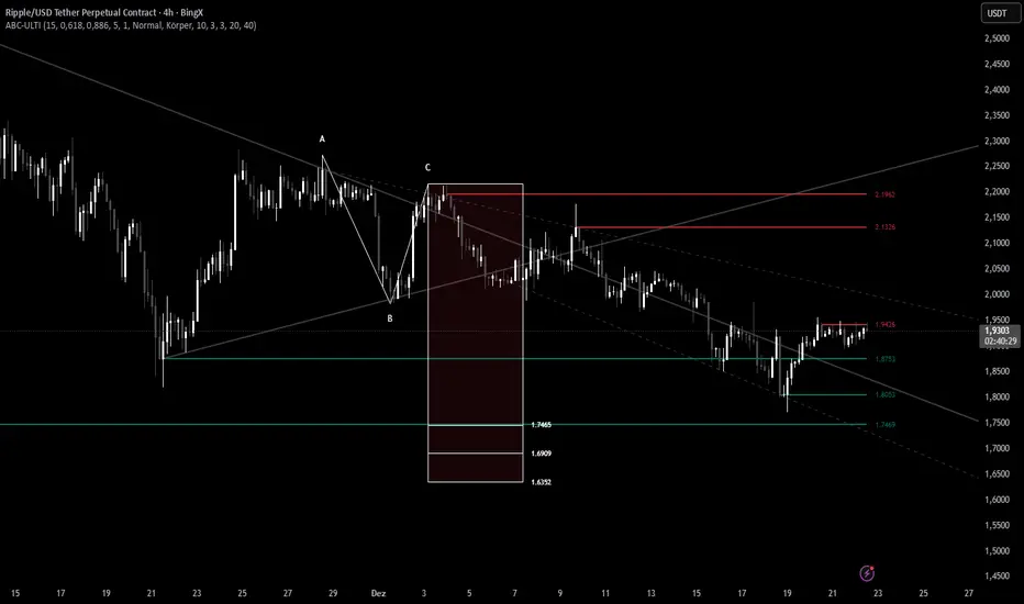
XABCD Harmonic Pattern Custom Range Interactive█ OVERVIEW
This indicator was designed based on Harmonic Pattern Book written by Scott Carney. It was simplified to user who may always used tools such as XABCD Pattern and Long Position / Short Position, which consume a lot of time, recommended for both beginner and expert of Harmonic Pattern Traders. XABCD Pattern require tool usage of Magnet tool either Strong Magnet, Week Magnet or none, which cause error or human mistake especially daily practice.
Simplified Guideline by sequence for Harmonic Pattern if using manual tools :
Step 1 : Trade Identification - XABCD Pattern
Step 2 : Trade Execution - Any manual tools of your choice
Step 3 : Trade Management - Position / Short Position
█ INSPIRATION
Inspired by design, code and usage of CAGR. Basic usage of custom range / interactive, pretty much explained here . Credits to TradingView.
I use a lot of XABCD Pattern and Long Position / Short Position, require 5 to 10 minutes on average, upon determine the validity of harmonic pattern.
Upon creating this indicator, I believed that time can be reduced, gain more confidence, reduce error during drawing XABCD, which helps most of harmonic pattern users.
█ FEATURES
Table can positioned by any postion and font size can be resized.
Table can be display through optimized display or manual control.
Validility of harmonic pattern depends on BC ratio.
Harmonic pattern can be displayed fully or optimized while showing BC ratio validity.
Trade Execution at point D can be displayed on / off.
Stop Loss and Take Profit can be calculated automatically or manually.
Optimized table display based extend line setup and profit and loss setup.
Execution zone can be offset to Point C, by default using Point D.
Currency can be show or hide.
Profit and Loss can be displayed on axis once line is extended.
█ HOW TO USE
Step 1 : Trade Identification - Draw points from Point X to Point C. Dont worry about magnet, point will attached depends on High or Low of the candle.
Step 2 : Trade Execution - Check the validity of BC to determine the validity of harmonic pattern generated. Pattern only generate 1 pattern upon success. Otherwise, redraw to other points.
Step 3 : Trade Management - Determine the current candle either reach Point D or Potential Reversal Zone (PRZ). Check for Profit & Loss once reach PRZ.
█ USAGE LIMITATIONS
Harmonic Patterns only limits to patterns mentioned in Harmonic Trading Volume 3 due to other pattern may have other or different philosophy.
Only can be used for Daily timeframe and below due to bar_time is based on minutes by default.
Not recommended for Weekly and Monthly timeframe.
If Point X, A, B, C and D is next to each other, it is recommend to use lower timeframe.
Automated alert is not supported for this release. However, alert can be done manually. Alert will updated on the version.
█ PINE SCRIPT LIMITATIONS
Known bug for when calculate time in array, causing label may not appeared or offset.
Unable to convert to library due to usage of array.get(). I prefer usage for a combination of array.get(id, 0), array.get(id, 1), array.get(id, 2) into custom function, however I faced this issue during make arrays of label. Index can be simply refered as int, for id, i not sure, already try id refered as simple, nothing happens.
linefill.new() will appeared as diamond box if overused.
Text in box.new() unable to use ternary condition or switch to change color. Bgcolor also affected.
Label display is larger than XABCD tool. Hopefully in future, have function to resize label similar to XABCD tools.
█ IMPORTANTS
Trade Management (Profit & Loss) is calculated from Point A to D.
Take Profit is calculated based on ratio 0.382 and 0.618 of Point A to D.
Always check BC validity before proceed to Trade Management.
Length of XABCD is equal to XAB plus BCD, where XAB and BCD are one to one ratio. Length is measured in time.
Use other oscillator to countercheck. Normally use built-in Relative Strength Index (RSI) and Divergence Indicator to determine starting point of Point X and A.
█ HARMONIC PATTERNS SUPPORTED
// Credits to Scott M Carney, author of Harmonic Trading Volume 3: Reaction vs. Reversal
Alt Bat - Page 101
Bat - Page 98
Crab - Page 104
Gartley - Page 92
Butterfly - Page 113
Deep Crab - Page 107
Shark - Page 119 - 220
█ FAQ
Pattern such as 5-0, perfect XABCD and ABCD that not included, will updated on either next version or new release.
Point D time is for approximation only, not including holidays and extended session.
Basic explaination for Harmonic Trading System (Trade Identification, Trade Execution and Trade Management).
Harmonic Patterns values is pretty much summarized here including Stop Loss.
Basic explanation for Alt Bat, Bat, Crab, Gartley, Deep Crab and Butterfly.
█ USAGE / TIPS EXAMPLES (Description explained in each image)
在脚本中搜索"harmonic"

Spread by//Every spread & central tendency measure in 1 script with comfortable visualization, including scrips's status line.
Spread measures:
- Standard deviation (for most cases);
- Average deviation (if there are extreme values);
- GstDev - Geometric Standard Deviation (exclusively for Geometric Mean);
- HstDev - Harmonic Deviation (exclusively for Harmonic Mean).
These modified functions will calculate everything right, they will take source, length, AND basis of your choice, unlike the ones from TW.
Central tendency measures:
- Mean (if everything's cool & equal);
- Median (values clustering towards low/high part of the rolling window);
- Trimean (3/more distinguishable clusters of data);
- Midhinhe (2 distinguishable clusters of data);
- Geometric Mean ( |low.. ... ... .. .... ... . . . . . . . . . . . .high| this kinda data); <- Exp law
- Harmonic Mean { |low. . . . . . . . . . . . . . .. . . .high| kinda data). <- Reciprocal law
Listen:
1) Don't hesitate using Standard Deviation with non-mean, like "Midhinge Standard Devition", despite what ol' stats gurus gonna say, it works when it's appropriate;
2) Don't check log space while using Geometric Mean & Geometric Standard Deviation, these 2 implement log stuff by design, I mean unless u wanna make it double xd
3) You can use this script, modify it how you want, ask me questions whatever, just make money using it;
4) Use Midrange & Midpoints in tandem when data follows ~addition law (like this . . . . . . . . . . . . . . . . . . . . .). <- just addition law
Look at the data, choose spread measure first, then choose central tendency measure, not vice versa.
!!!
Ain't gonna place ® sign on standard deviations like one B guy did in 1980s lmao, but if your wanna use Harmonic Deviations in science/write about/cite it/whatever, pls give me a lil credit at least, I've never seen it anywhere and unfortunately had to develop it by myself. it's useful when your data develops by reciprocals law (opposite to exponential).
Peace TW

BTC Gann Harmonics Weighted + Phase + EMA OptimizedBTC Gann Harmonics Weighted + Phase + EMA Optimized

Complete Harmonic PatternOverview:
The ultimate harmonic XABCD pattern identification, prediction, and backtesting system.
Harmonic patterns are among the most accurate of trading signals, yet they're widely underutilized because they can be difficult to spot and tedious to validate. If you've ever come across a pattern and struggled with questions like "are these retracement ratios close enough to the harmonic ratios?" or "what are the Potential Reversal levels and are they confluent with point D?", then this tool is your new best friend. Or, if you've never traded harmonic patterns before, maybe it's time to start. Put away your drawing tools and calculators, relax, and let this indicator do the heavy lifting for you.
- Identification -
An exhaustive search across multiple pivot lengths ensures that even the sneakiest harmonic patterns are identified. Each pattern is evaluated and assigned a score, making it easy to differentiate weak patterns from strong ones. Tooltips under the pattern labels show a detailed breakdown of the pattern's score and retracement ratios (see the Scoring section below for details).
- Prediction -
After a pattern is identified, paths to potential targets are drawn, and Potential Reversal Zone (PRZ) levels are plotted based on the retracement ratios of the harmonic pattern. Targets are customizable by pattern type (e.g. you can specify one set of targets for a Gartley and another for a Bat, etc).
- Backtesting -
A table shows the results of all the patterns found in the chart. Change your target, stop-loss, and % error inputs and observe how it affects your success rate.
//------------------------------------------------------
// Scoring
//------------------------------------------------------
A percentage-based score is calculated from four components:
(1) Retracement % Accuracy - this measures how closely the pattern's retracement ratios match the theoretical values (fibs) defined for a given harmonic pattern. You can change the "Allowed fib ratio error %" in Settings to be more or less inclusive.
(2) PRZ Level Confluence - Potential Reversal Zone levels are projected from retracements of the XA and BC legs. The PRZ Level Confluence component measures the closeness of the closest XA and BC retracement levels, relative to the total height of the PRZ.
(3) Point D / PRZ Confluence - this measures the closeness of point D to either of the closest two PRZ levels (identified in the PRZ Level Confluence component above), relative to the total height of the PRZ. In theory, the closer together these levels are, the higher the probability of a reversal.
(4) Leg Length Symmetry - this measures the ΔX symmetry of each leg. You can change the "Allowed leg length asymmetry %" in settings to be more or less inclusive.
So, a score of 100% would mean that (1) all leg retracements match the theoretical fib ratios exactly (to 16 decimal places), (2) the closest XA and BC PRZ levels are exactly the same, (3) point D is exactly at the confluent PRZ level, and (4) all legs are exactly the same number of bars. While this is theoretically possible, you have better odds of getting struck by lightning twice on a sunny day.
Calculation weights of all four components can be changed in Settings.
//------------------------------------------------------
// Targets
//------------------------------------------------------
A hard-coded set of targets are available to choose from, and can be applied to each pattern type individually:
(1) .618 XA = .618 retracement of leg XA, measured from point D
(2) 1.272 XA = 1.272 retracement of leg XA, measured from point D
(3) 1.618 XA = 1.618 retracement of leg XA, measured from point D
(4) .618 CD = .618 retracement of leg CD, measured from point D
(5) 1.272 CD = 1.272 retracement of leg CD, measured from point D
(6) 1.618 CD = 1.618 retracement of leg CD, measured from point D
(7) A = point A
(8) B = point B
(9) C = point C

Lorentzian Harmonic Flow - Temporal Market Dynamic Lorentzian Harmonic Flow - Temporal Market Dynamic (⚡LHF)
By: DskyzInvestments
What this is
LHF Pro is a research‑grade analytical instrument that models market time as a compressible medium , extracts directional flow in curved time using heavy‑tailed kernels, and consults a history‑based memory bank for context before synthesizing a final, bounded probabilistic score . It is not a mashup; each subsystem is mathematically coupled to a single clock (time dilation via gamma) and a single lens (Lorentzian heavy‑tailed weighting). This script is dense in logic (and therefore heavy) because it prioritizes rigor, interpretability, and visual clarity.
Intended use
Education and research. This tool expresses state recognition and regime context—not guarantees. It does not place orders. It is fully functional as published and contains no placeholders. Nothing herein is financial advice.
Why this is original and useful
Curved time: Markets do not move at a constant pace. LHF Pro computes a Lorentz‑style gamma (γ) from relative speed so its analytical windows contract when the tape accelerates and relax when it slows.
Heavy‑tailed lens: Lorentzian kernels weight information with fat tails to respect rare but consequential extremes (unlike Gaussian decay).
Memory of regimes: A K‑nearest‑neighbors engine works in a multi‑feature space using Lorentz kernels per dimension and exponential age fade , returning a memory bias (directional expectation) and assurance (confidence mass).
One ecosystem: Squeeze, TCI, flow, acceleration, and memory live on the same clock and blend into a single final_score —visualized and documented on the dashboard.
Cognitive map: A 2D heat map projects memory resonance by age and flow regime, making “where the past is speaking” visible.
Shadow portfolio metaphor: Neighbor outcomes act like tiny hypothetical positions whose weighted average forms an educational pressure gauge (no execution, purely didactic).
Mathematical framework (full transparency)
1) Returns, volatility, and speed‑of‑market
Log return: rₜ = ln(closeₜ / closeₜ₋₁)
Realized vol: rv = stdev(r, vol_len); vol‑of‑vol: burst = |rv − rv |
Speed‑of‑market (analog to c): c = c_multiplier × (EMA(rv) + 0.5 × EMA(burst) + ε)
2) Trend velocity and Lorentz gamma (time dilation)
Trend velocity: v = |close − close | / (vel_len × ATR)
Relative speed: v_rel = v / c
Gamma: γ = 1 / √(1 − v_rel²), stabilized by caps (e.g., ≤10)
Interpretation: γ > 1 compresses market time → use shorter effective windows.
3) Adaptive temporal scale
Adaptive length: L = base_len / γ^power (bounded for safety)
Harmonic horizons: Lₛ = L × short_ratio, Lₘ = L × mid_ratio, Lₗ = L × long_ratio
4) Lorentzian smoothing and Harmonic Flow
Kernel weight per lag i: wᵢ = 1 / (1 + (d/γ)²), d = i/L
Horizon baselines: lw_h = Σ wᵢ·price / Σ wᵢ
Z‑deviation: z_h = (close − lw_h)/ATR
Harmonic Flow (HFL): HFL = (w_short·zₛ + w_mid·zₘ + w_long·zₗ) / (w_short + w_mid + w_long)
5) Flow kinematics
Velocity: HFL_vel = HFL − HFL
Acceleration (curvature): HFL_acc = HFL − 2·HFL + HFL
6) Squeeze and temporal compression
Bollinger width vs Keltner width using L
Squeeze: BB_width < KC_width × squeeze_mult
Temporal Compression Index: TCI = base_len / L; TCI > 1 ⇒ compressed time
7) Entropy (regime complexity)
Shannon‑inspired proxy on |log returns| with numerical safeguards and smoothing. Higher entropy → more chaotic regime.
8) Memory bank and Lorentzian k‑NN
Feature vector (5D):
Outcomes stored: forward returns at H5, H13, H34
Per‑dimension similarity: k(Δ) = 1 / (1 + Δ²), weighted by user’s feature weights
Age fading: weight_age = mem_fade^age_bars
Neighbor score: sᵢ = similarityᵢ × weight_ageᵢ
Memory bias: mem_bias = Σ sᵢ·outcomeᵢ / Σ sᵢ
Assurance: mem_assurance = Σ sᵢ (confidence mass)
Normalization: mem_bias normalized by ATR and clamped into band
Shadow portfolio metaphor: neighbors behave like micro‑positions; their weighted net forward return becomes a continuous, adaptive expectation.
9) Blended score and breakout proxy
Blend factor: α_mem = 0.45 + 0.15 × (γ − 1)
Final score: final_score = (1−α_mem)·tanh(HFL / (flow_thr·1.5)) + α_mem·tanh(mem_bias_norm)
Breakout probability (bounded): energy = cap(TCI−1) + |HFL_acc|×k + cap(γ−1)×k + cap(mem_assurance)×k; breakout_prob = sigmoid(energy). Caps avoid runaway “100%” readings.
Inputs — every control, purpose, mechanics, and tuning
🔮 Lorentz Core
Auto‑Adapt (Vol/Entropy): On = L responds to γ and entropy (breathes with regime), Off = static testing.
Base Length: Calm‑market anchor horizon. Lower (21–28) for fast tapes; higher (55–89+) for slow.
Velocity Window (vel_len): Bars used in v. Shorter = more reactive γ; longer = steadier.
Volatility Window (vol_len): Bars used for rv/burst (c). Shorter = more sensitive c.
Speed‑of‑Market Multiplier (c_multiplier): Raises/lowers c. Lower values → easier γ spikes (more adaptation). Aim for strong trends to peak around γ ≈ 2–4.
Gamma Compression Power: Exponent of γ in L. <1 softens; >1 amplifies adaptation swings.
Max Kernel Span: Upper bound on smoothing loop (quality vs CPU).
🎼 Harmonic Flow
Short/Mid/Long Horizon Ratios: Partition L into fast/medium/slow views. Smaller short_ratio → faster reaction; larger long_ratio → sturdier bias.
Weights (w_short/w_mid/w_long): Governs HFL blend. Higher w_short → nimble; higher w_long → stable.
📈 Signals
Squeeze Strictness: Threshold for BB1 = compressed (coiled spring); <1 = dilated.
v/c: Relative speed; near 1 denotes extreme pacing. Diagnostic only.
Entropy: Regime complexity; high entropy suggests caution, smaller size, or waiting for order to return.
HFL: Curved‑time directional flow; sign and magnitude are the instantaneous bias.
HFL_acc: Curvature; spikes often accompany regime ignition post‑squeeze.
Mem Bias: Directional expectation from historical analogs (ATR‑normalized, bounded). Aligns or conflicts with HFL.
Assurance: Confidence mass from neighbors; higher → more reliable memory bias.
Squeeze: ON/RELEASE/OFF from BB

Quantum Harmonic Oscillator Overlay🧪 Quantum Harmonic Oscillator Overlay
A visual model of price behavior using quantum harmonic oscillation principles
📜 Indicator Overview
The Quantum Harmonic Oscillator Overlay applies concepts from both classical physics (harmonic motion) and quantum mechanics (energy states) to model and visualize how price orbits around a central trend line. It overlays a Linear Regression line (representing the “mean position” or ground state of price) and calculates surrounding energy levels (σ-zones) akin to quantum shells that price can "jump" between.
This indicator is particularly useful for visualizing mean reversion, volatility compression/expansion, and momentum-driven price breakthroughs.
🧠 Core Concepts
Linear Regression Line (LSR): This is the calculated center of gravity or equilibrium path of price over a user-defined period. Think of it like the lowest energy state or central axis around which price vibrates.
Standard Deviation Zones (σ-levels):
1σ: The majority of normal price activity; within this range, price tends to fluctuate if in balance.
2σ: Indicates volatility or possible breakout pressure.
3σ: Represents extreme movement — a phase shift in energy, potentially leading to reversal or continuation with higher momentum.
Quantum Analogy: Just like in a quantum harmonic oscillator, particles (here, prices) move probabilistically between discrete energy states. The further the price moves from the center, the more "energy" (momentum, volume, volatility) is implied.
⚙️ Input Parameters
Setting Description
Linear Regression Length The number of bars used to calculate the regression trend (default 100). Affects the central path and responsiveness.
σ Multipliers (1σ, 2σ, 3σ) Determine how far each band is from the regression line. Adjusting these can highlight different price behaviors.
Show Energy Level Zones Toggle visibility of the colored bands around the regression line.
Show LSR Center Line Toggles visibility of the white Linear Regression line itself.
🎨 Visual Components
Color Zone Interpretation
✅ Green ±1σ Normal oscillation / mean reversion area. Ideal for range-bound strategies.
🟧 Orange ±2σ Warning zone; price may be gaining momentum or volatility.
🔴 Red ±3σ High-momentum state or anomaly. These regions may imply trend exhaustion, reversals, or breakouts.
White Line: The LSR — the average trajectory of the price movement.
Pink Dots: Appear when price exceeds Zone 3 (outside ±3σ) — a signal of extreme behavior or a possible regime shift.
📈 How to Use This Indicator
1. Detect Overextensions
When price touches or breaches the 3σ zone, it is likely overextended. This can be used to anticipate potential snapbacks or strong breakout trends.
2. Identify Mean Reversion Trades
If price exits the 2σ or 3σ zones and returns toward the center line, this signals a likely mean reversion setup.
3. Volatility Compression or Expansion
Flat zones between σ levels suggest calm markets; widening bands suggest expanding volatility.
4. Use with Confirmation Tools
Combine with momentum oscillators (MACD, RSI) or volume-based signals to confirm reversals or continuation outside Zone 3.
🔮 Philosophical Note
This indicator embodies the metaphor that the market behaves like a quantum oscillator — price particles exist in a probabilistic field and jump between discrete zones of volatility and energy. Tracking these transitions allows the trader to see price behavior as rhythmic, wave-like, and multidimensional rather than purely linear.

ABCD Projection [Trendoscope®]Over the years, we have extensively explored and published numerous scripts centered around various chart patterns, including Harmonic Patterns, Reversal Patterns, Elliott Waves, and more. Our expertise in these areas has led to frequent requests for an indicator based on the ABCD pattern. Although we didn't include it as part of our Harmonic Patterns collection, the development of a dedicated ABCD Projection Indicator has always been a priority for us.
🎲 Overview of the ABCD Projection Indicator
The ABCD Projection Indicator is designed to identify and project ABCD patterns using a Zigzag-based approach. This pattern, characterized by alternating pivot highs and lows labeled as A, B, C, and D, is particularly significant in trending markets where it signifies trend continuation following deep pullbacks.
The indicator works by confirming the ABC pivots and projecting the D pivot based on the established price swings. Since ABCD patterns are most effective in trending environments, the indicator focuses on filtering patterns where the retracement from the C pivot has not compromised the trade's potential. Specifically, it ensures that the starting point (S)—where the pattern is detected—has not retraced beyond a defined threshold, preserving the opportunity to execute a trade with the goal of reaching the projected D pivot.
Additionally, the ABCD Projection Indicator considers the retracement ratio from the C pivot, which plays a crucial role in risk management. A higher retracement ratio reduces the stop distance (from pivot A to the entry point S) while increasing the distance to the target (pivot D), thereby enhancing the reward/risk ratio for trades.
🎲 Components of the ABCD Projection Indicator
The ABCD Projection Indicator comprises several key components:
A, B, C Pivots and Zigzag Wave : These elements form the foundational structure of the ABCD pattern.
S Point : This is the location where the pattern is identified, positioned a few bars away from the confirmed C pivot.
Estimated D Pivot : The D pivot is projected based on the A, B, and C price levels. The time or distance to the D pivot is influenced by the starting point S.
Mini Stats Table : Located in the top right corner, this table displays win/loss ratios and risk/reward data for both bullish and bearish scenarios.
Fibonacci Levels : Calculated from the C to D pivots, these levels are provided as a reference for additional analysis.
🎲 Indicator Settings
The settings for the ABCD Projection Indicator are minimal and intuitive, with tooltips provided to guide users through the configuration process.

Multi-Timeframe Recursive Zigzag [Trendoscope®]🎲 Welcome to the Advanced World of Zigzag Analysis
Embark on a journey through the most comprehensive and feature-rich Zigzag implementation you’ll ever encounter. Our Multi-Timeframe Recursive Zigzag Indicator is not just another tool; it's a groundbreaking advancement in technical analysis.
🎯 Key Features
Multi Time-Frame Support - One of the rare open-source Zigzag indicators with robust multi-timeframe capabilities, this feature sets our tool apart, enabling a broader and more dynamic market analysis.
Innovative Recursive Zigzag Algorithm - At its core is our unique Recursive Zigzag Algorithm, a pioneering development that powers multiple Zigzag levels, offering an intricate view of market movements. This proprietary algorithm is the backbone of our advanced pattern recognition indicators.
Sub-Waves and Micro-Waves Analysis - Dive deeper into market trends with our Sub-Waves and Micro-Waves feature. Sub-Waves reveal the interconnectedness of various Zigzag levels, while Micro-Waves offer insight into the fundamental waves at the base level.
Enhanced Indicator Tracking - Integrate and track your custom indicators or oscillators with the zigzag, capturing their values at each Zigzag level, complete with retracement ratios. This offers a comprehensive view of market dynamics.
Curved Zigzag Visualization - Experience a new way of visualizing market movements with our Curved Zigzag Display, employing Pine Script’s polyline feature for a more intuitive and visually appealing representation.
Built-in Customizable Alerts - Stay ahead with built-in alerts that can be customized via user input settings.
🎯 Practical Applications
Our Zigzag Indicator is designed with an understanding of its inherent nature - the last unconfirmed pivot that consistently repaints. This characteristic, while by design, directs its usage more towards pattern recognition rather than direct identification of market tops and bottoms. Here's how you can leverage the Zigzag Indicator:
Harmonic Patterns - Ideal for those familiar with harmonic patterns, this tool simplifies the manual spotting of complex XABCD, ABC, and ABCD patterns on charts.
Chart Patterns - Effortlessly identify patterns like Double/Triple Taps, Head and Shoulders, Inverse Head and Shoulders, and Cup and Handle patterns with enhanced clarity. Navigate through challenging patterns such as Triangles, Wedges, Flags, and Price Channels, where the Zigzag Indicator adds a layer of precision to your breakout strategy.
Elliott Wave Components - The indicator's detailed pivot highlighting aids in identifying key Elliott Wave components, enhancing your wave analysis and decision-making process.
🎲 Deep Dive into Indicator Features
Join us as we explore the intricate features of our indicator in more detail.
🎯 Multi-Timeframe Capability
Our indicator comes equipped with an input option for selecting the desired resolution. This unique feature allows users to view higher timeframe Zigzag patterns directly on their lower timeframe charts.
🎯 Recursive Multi Level Zigzag
Our advanced recursive approach creates multi-level Zigzags from lower-level data. For instance, the level 0 Zigzag forms the base, calculated from specified length and depth parameters, while level 1 Zigzag is derived using level 0 as its foundation, and so forth.
The indicator not only displays multiple Zigzag levels but also offers settings to emphasize specific levels for more detailed analysis.
🎯 Sub-Components and Micro-Components of Zigzag Wave
Sub-components within a Zigzag wave consist of the previous level's Zigzag pivots. Meanwhile, the micro-components are composed of the base level (Level 0) Zigzag pivots encapsulated within the wave.
🎯 Curved Zigzag
Experience a new perspective with our curved Zigzag display. This innovative feature utilizes the polyline curved option to automatically generate sinusoidal waves based on multiple points.
🎯 Indicator Tracking
Default indicators such as RSI, MFI, and OBV are included, alongside the ability to track one external indicator at each Zigzag pivot.
🎯 Customizable Alerts
Our indicator employs the `alert()` function for alert creation. While this means the absence of a customization text box in the alert settings, we've included a custom text area for users to create their own alert templates.
Template placeholders include:
{alertType} - type of alert. Either Confirmed Pivot Update or Last Pivot Update. Depends on the alert type selected in the inputs.
When Last Pivot Update type is selected, the alerts are triggered whenever there is a new Zigzag Pivot. This may also be a repaint of last unconfirmed pivot.
When Confirmed Pivot Update type is selected, the alerts are triggered only when a pivot becomes a confirmed pivot.
{level} - Zigzag level on which the alert is triggered.
{pivot} - Details of the last pivot or confirmed pivot including price, ratio, indicator values and ratios, subcomponent and micro-component pivots.
🎲 User Settings Overview
🎯 Zigzag and Generic Settings
This involves some generic zigzag calculation settings such as length, depth, and timeframe. And few display options such as theme, Highlight Level and Curved Zigzag. By default, zigzag calculation is done based on the latest real time bar. An option is provided to disable this and use only confirmed bars for the calculation.
Indicator Settings
Allows users to track one or more oscillators or volume indicators. Option to add any indicator via external input is provided.
🎯 Alert Settings
Has input fields required to select and customize alerts.

Custom XABCD Validation and Backtesting ToolOverview:
We hear a lot about Gartleys, bats, crabs and the rest of the barnyard crew, but have you ever wondered what other creatures might be lurking out there yet to be discovered? Well wonder no longer, it's time to find out for yourself! The Custom XABCD Validation and Backtesting Tool allows you to define retracement ratios and targets for your very own patterns.
Tips:
(1) Adjust the patterns entry/stop/target configuration and see how it affects the pattern's backtesting results.
(2) Adjust the weights of pattern score components (% error, PRZ confluence, Point D/PRZ confluence), along with the entry minimum score requirements ('If score is above'), and see how it affects the patterns' results.
Pattern Scoring:
The pattern's score is an attempt to represent the quality of a pattern with a single metric. This is one of the most powerful aspects of the tool because it can quickly tell you whether a trade is worth entering. The score is based on 3 components:
(1) Retracement % Accuracy - this measures how closely a pattern's retracement ratios match your defined theoretical values. You can change the "Allowed ratio error %" in Settings to be more or less inclusive.
(2) PRZ Level Confluence - Potential Reversal Zone levels are retracements of the XA, BC, and/or XC legs. These levels indicate where a potential reversal might occur (i.e. pivot point D). The PRZ Level Confluence component measures the closeness of the two closest PRZ levels, relative to the height of the of the XA leg.
(3) Point D / PRZ Confluence - this measures the closeness of point D to either of the two closest PRZ levels (identified in the PRZ Level Confluence component above), relative to the height of the XA leg. In theory, the closer together these levels are, the higher the probability of a reversal.
While the score is percentage-based, it should not be confused with a probability. A score of 96% does not imply a 96% chance of success. It simply represents the average of the three components mentioned above, weighted according to the defined weight parameters. A score of 100% would mean that (1) all leg retracements match the defined theoretical retracement ratios exactly, (2) all PRZ retracement levels are exactly the same value, and (3) pivot point D occurred exactly at the confluent PRZ level.
Pattern scoring research has been ongoing since I introduced the concept with my Harmonic Pattern Detection, Prediction and Backtesting Tool (see below). So the way that the score is calculated is subject to change based on the results of that research.

HarmonicCalculation█ OVERVIEW
This library is complementary for XABCD Harmonic Pattern Custom Range Interactive
PriceDiff()
: Price Difference
Parameters:
: : price_1, price_2
Returns: : PriceDiff
TimeDiff()
: Time Difference
Parameters:
: : time_1, time_2
Returns: : TimeDiff
ReturnIndexOf3Arrays()
: Return Index Of 3 Arrays
Parameters:
: : id1, id2, id3, _int
Returns: : ReturnIndexOf3Arrays
AbsoluteRange()
: Price Difference
Parameters:
: : price, y, point
Returns: : AbsoluteRange
PriceAverage()
: To calculate average of 2 prices
Parameters:
: : price_1, price_2
Returns: : PriceAverage
TimeAverage()
: To calculate average of 2 times
Parameters:
: : time_1, time_2
Returns: : TimeAverage
StringBool()
: To show ratio in 3 decimals format
Parameters:
: : _value, _bool, _text
Returns: : StringBool
PricePercent()
: To show Price in percent format
Parameters:
: : _price, PriceRef, str_dir
Returns: : PricePercent
BoolCurrency()
: To show syminfo.currency
Parameters:
: : _bool
Returns: : BoolCurrency
RatioText()
: To show RatioText in 3 decimals format
Parameters:
: : _value, _text
Returns: : RatioText
RangeText()
: To display RangeText in Harmonic Range Format
Parameters:
: : _id1, _id2, _int, _text
Returns: : RangeText
PriceCurrency()
: To show Currency in Price Format
Parameters:
: : _bool, _value
Returns: : PriceCurrency
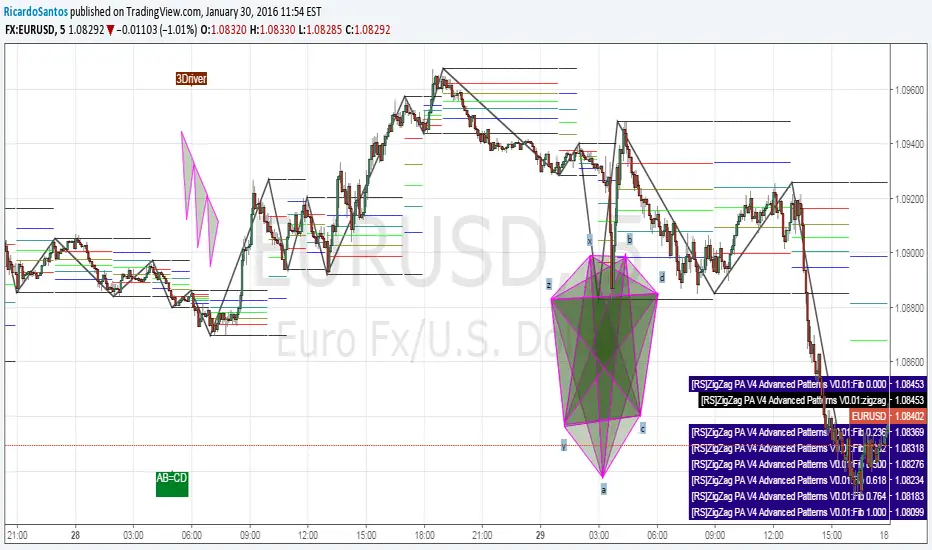
[RS]ZigZag PA V4 Advanced Patterns V0.01EXPERIMENTAL:
Method for detecting 4/5/6/7 point harmonics
included 3drive detection rates are rudimentary.
Dual Harmonic-based AHR DCA (Default :BTC-ETH)A panel indicator designed for dual-asset BTC/ETH DCA (Dollar Cost Averaging) decisions.
It is inspired by the Chinese community indicator "AHR999" proposed by “Jiushen”.
How to use:
Lower HM-based AHR → cheaper (potential buy zone).
Higher HM-based AHR → more expensive (potential risk zone).
Higher than Risk Threshold → consider to sell, but not suitable for DCA.
When both AHR lines are below the Risk threshold → buy the cheaper one (or split if similar).
If one AHR is above Risk → buy the other asset.
If both are above Risk → simulation shows “STOP (both risk)”.
Not limited to BTC/ETH — you can freely change symbols in the input panel
to build any dual-asset DCA pair you want (e.g., BTC/BNB, ETH/SOL, etc.).
What you’ll see:
Two lines: AHR BTC (HM) and AHR ETH (HM)
Two dashed lines: OppThreshold (green) and RiskThreshold (red)
Colored fill showing which asset is cheaper (BTC or ETH)
Buy markers:
- B = Buy BTC
- E = Buy ETH
- D = Dual (split budget)
Top-right table: prices, AHRs, thresholds, qOpp/qRisk%, simulation, P&L
Labels showing last-bar AHR values
Core idea:
Use an AHR based on Harmonic Moving Average (HM) — a ratio that measures how “cheap or expensive” price is relative to both its short-term mean and long-term trend.
The original AHR999 used SMA and was designed for BTC only.
This indicator extends it with cross-exchange percentile mapping, allowing the empirical “opportunity/risk” zones of the AHR999 (on Bitstamp) to adapt automatically to the current market pair.
The indicator derives two adaptive thresholds:
OppThreshold – opportunity zone
RiskThreshold – risk zone
These thresholds are compared with the current HM-based AHR of BTC and ETH to decide which asset is cheaper, and whether it is good to DCA or not, or considering to sell(When it in risk area).
This version uses
Display base: Binance (default: perpetual) with HM-based AHR
Percentile base: Bitstamp spot SMA-AHR (complete, stable history)
Rolling window: 2920 daily bars (~8 years) for percentile tracking
Concept summary
AHR measures the ratio of price to its long-term regression and short-term mean.
HM replaces SMA to better reflect equal-fiat-cost DCA behavior.
Cross-exchange percentile mapping (Bitstamp → Binance) keeps thresholds consistent with the original AHR999 interpretation.
Recommended settings (1D):
DCA length (harmonic): 200
Log-regression lookback: 1825 (≈5 years)
Rolling window: 2920 (≈8 years)
Reference thresholds: 0.45 / 1.20 (AHR999 empirical priors)
Tie split tolerance (ΔAHR): 0.05
Daily budget: 15 USDT (simulation)
All display options can be toggled: table, markers, labels, etc.
Notes:
When the rolling window is filled (2920 bars by default), thresholds are first calculated and then visually backfilled as left-extended lines.
The “buy markers” and “decision table” are light simulations without fees or funding costs — for rhythm and relative analysis, not backtesting.

---Advanced Harmonic Pattern Scanner v5Summary of the Script:
All Patterns Covered: The script includes all major harmonic patterns: Butterfly, Gartley, Crab, Bat, Cypher, and Three Drives. Both bullish and bearish versions are detected.
ZigZag Swings: The zigzag logic helps find swing points (X, A, B, C, D) which are essential for forming these patterns. You can adjust the zigzagDepth parameter to fine-tune how sensitive the pattern detection is to price swings.
Fibonacci Levels: Each pattern uses specific Fibonacci retracement or extension levels to identify potential patterns, and the script compares price movements to these ratios.
Visual Aid: It uses plotshape() to display detected patterns on the chart and optional line.new() functions to connect the swing points for a better visual representation of the patterns.
How to Customize:
Timeframe: You can run this script on different timeframes by changing the chart on TradingView (1 min, 1 hour, 1 day, etc.).
ZigZag Sensitivity: Adjust the zigzagDepth to refine how frequently swing points are detected. Larger numbers will reduce sensitivity and show fewer but more pronounced patterns.
Pattern Refinement: Modify Fibonacci levels to experiment with custom harmonic patterns or adjust thresholds for the existing ones.
This code is an advanced version and scans the market comprehensively for all major harmonic patterns. Let me know if you need further modifications or explanations!

[fikira] Harmonic Patterns 1When using "Harmonic Patterns", always look at the bigger picture, please do not depend solely on the "Pattern".
Use other indicators,... to confirm what you think is going on!
That said, it is quite useful!
Beside my "The Gartley", now, OPEN SOURCE, we have "Harmonic Patterns" in 2 parts (otherwise many lines are gone because the script is too large)
- ABCD
- Gartley
- Cypher
- 5.0
A "Pattern" is created by checking 5 consecutive ( pivot ) points, starting with X, A, B, C, and ending with point D.
At point D all 5 points are compared, calculated and verified.
When confirmed, a "Label" will be plotted at point D, together with the "Entry", "Take Profit" and "Stop Loss" price.
The "Entry", "Take Profit" and "Stop Loss" lines will be plotted as well at point D.
Lastly, a "Drawing" automatically will be displayed which makes the "Pattern" visible.
Please do mind, the "Drawing" is calculated differently, the "Drawing" sometimes can be displayed incorrectly
when prices are too close to each other (for example low Satoshi price changes).
THE "ENTRY", "TAKE PROFIT", "STOP LOSS" PRICES AND LINES ARE NOT AFFECTED AT ALL BY THIS, THEY WILL SHOW CORRECTLY!
- 1 "TP point" can be changed ("TP Level 0.618")
- "Labels", "Lines", "Drawings" can be disabled/enabled
- "Labels" can be made smaller or bigger ("Size Label")
- "Labels" can be placed further or closer to the bar ("Distance TP Label" > higher = closer, lower = further)
- "Lines" can be made thicker or thinner ("TP Linewidth")
- "Drawings" can be made thicker or thinner ("Drawings Linewidth")
- "Drawings" are created by comparing with 100 bars back in history (default), should it be (very rarely) a triangle is displayed flat on the left side,
possibly the first point(s) is/are further than 100 bars ago, in this case increase "Period Drawings" above 100.
- When several "Patterns" appear on the chart, the oldest ones won't be displayed anymore, first the "Drawings", then the "Lines"
The last (present) ones will always be displayed in total without a problem!
- If you want to see "Patterns" with less correct measurement, change "Error Marge" 0.9 - 1" and "Error Marge" 1 - 1.1"), this gives max. about 10% extra margin
- Added more settings regarding "Drawing Lines"
Thank you very much!
Auto Fibonacci Bands for HarmonicAuto Fibonacci Bands for Harmonic
Previous day's High-Low based Fibonnacci Retracement(today's open=0.5 line)
follow series -1.618/-0.618/-0.382/0/0.118/0.286/0.386/0.5/0.682/0.786/0.886/1/1.382/1.618/2.618
it's for Harmonic:)
ABC Pro Ultimate S/RABC Pro Ultimate is a high-precision trading tool designed to identify harmonic ABC (Zigzag) patterns and combine them with institutional Support & Resistance levels. Unlike standard indicators that clutter your chart with noise, this script filters for high-relevance pivot points from the distant past to provide truly meaningful trade setups.
Density Zones (GM Crossing Clusters) + QHO Spin FlipsINDICATOR NAME
Density Zones (GM Crossing Clusters) + QHO Spin Flips
OVERVIEW
This indicator combines two complementary ideas into a single overlay: *this combines my earlier Geometric Mean Indicator with the Quantum Harmonic Oscillator (Overlay) with additional enhancements*
1) Density Zones (GM Crossing Clusters)
A “Density Zone” is detected when price repeatedly crosses a Geometric Mean equilibrium line (GM) within a rolling lookback window. Conceptually, this identifies regions where the market is repeatedly “snapping” across an equilibrium boundary—high churn, high decision pressure, and repeated re-selection of direction.
2) QHO Spin Flips (Regression-Residual σ Breaches)
A “Spin Flip” is detected when price deviates beyond a configurable σ-threshold (κ) from a regression-based equilibrium, using normalized residuals. Conceptually, this marks excursions into extreme states (decoherence / expansion), which often precede a reversion toward equilibrium and/or a regime re-scaling.
These two systems are related but not identical:
- Density Zones identify where equilibrium crossings cluster (a “singularity”/anchor behavior around GM).
- Spin Flips identify when price exceeds statistically extreme displacement from the regression equilibrium (LSR), indicating expansion beyond typical variance.
CORE CONCEPTS AND FORMULAS
SECTION A — GEOMETRIC MEAN EQUILIBRIUM (GM)
We define two moving averages:
(1) MA1_t = SMA(close_t, L1)
(2) MA2_t = SMA(close_t, L2)
We define the equilibrium anchor as the geometric mean of MA1 and MA2:
(3) GM_t = sqrt( MA1_t * MA2_t )
This GM line acts as an equilibrium boundary. Repeated crossings are interpreted as high “equilibrium churn.”
SECTION B — CROSS EVENTS (UP/DOWN)
A “cross event” is registered when the sign of (close - GM) changes:
Define a sign function s_t:
(4) s_t =
+1 if close_t > GM_t
-1 if close_t < GM_t
s_{t-1} if close_t == GM_t (tie-breaker to avoid false flips)
Then define the crossing event indicator:
(5) crossEvent_t = 1 if s_t != s_{t-1}
0 otherwise
Additionally, the indicator plots explicit cross markers:
- Cross Above GM: crossover(close, GM)
- Cross Below GM: crossunder(close, GM)
These provide directional visual cues and match the original Geometric Mean Indicator behavior.
SECTION C — DENSITY MEASURE (CROSSING CLUSTER COUNT)
A Density Zone is based on the number of cross events occurring in the last W bars:
(6) D_t = Σ_{i=0..W-1} crossEvent_{t-i}
This is a “crossing density” score: how many times price has toggled across GM recently.
The script implements this efficiently using a cumulative sum identity:
Let x_t = crossEvent_t.
(7) cumX_t = Σ_{j=0..t} x_j
Then:
(8) D_t = cumX_t - cumX_{t-W} (for t >= W)
cumX_t (for t < W)
SECTION D — DENSITY ZONE TRIGGER
We define a Density Zone state:
(9) isDZ_t = ( D_t >= θ )
where:
- θ (theta) is the user-selected crossing threshold.
Zone edges:
(10) dzStart_t = isDZ_t AND NOT isDZ_{t-1}
(11) dzEnd_t = NOT isDZ_t AND isDZ_{t-1}
SECTION E — DENSITY ZONE BOUNDS
While inside a Density Zone, we track the running high/low to display zone bounds:
(12) dzHi_t = max(dzHi_{t-1}, high_t) if isDZ_t
(13) dzLo_t = min(dzLo_{t-1}, low_t) if isDZ_t
On dzStart:
(14) dzHi_t := high_t
(15) dzLo_t := low_t
Outside zones, bounds are reset to NA.
These bounds visually bracket the “singularity span” (the churn envelope) during each density episode.
SECTION F — QHO EQUILIBRIUM (REGRESSION CENTERLINE)
Define the regression equilibrium (LSR):
(16) m_t = linreg(close_t, L, 0)
This is the “centerline” the QHO system uses as equilibrium.
SECTION G — RESIDUAL AND σ (FIELD WIDTH)
Residual:
(17) r_t = close_t - m_t
Rolling standard deviation of residuals:
(18) σ_t = stdev(r_t, L)
This σ_t is the local volatility/width of the residual field around the regression equilibrium.
SECTION H — NORMALIZED DISPLACEMENT AND SPIN FLIP
Define the standardized displacement:
(19) Y_t = (close_t - m_t) / σ_t
(If σ_t = 0, the script safely treats Y_t = 0.)
Spin Flip trigger uses a user threshold κ:
(20) spinFlip_t = ( |Y_t| > κ )
Directional spin flips:
(21) spinUp_t = ( Y_t > +κ )
(22) spinDn_t = ( Y_t < -κ )
The default κ=3.0 corresponds to “3σ excursions,” which are statistically extreme under a normal residual assumption (even though real markets are not perfectly normal).
SECTION I — QHO BANDS (OPTIONAL VISUALIZATION)
The indicator optionally draws the standard σ-bands around the regression equilibrium:
(23) 1σ bands: m_t ± 1·σ_t
(24) 2σ bands: m_t ± 2·σ_t
(25) 3σ bands: m_t ± 3·σ_t
These provide immediate context for the Spin Flip events.
WHAT YOU SEE ON THE CHART
1) MA1 / MA2 / GM lines (optional)
- MA1 (blue), MA2 (red), GM (green).
- GM is the equilibrium anchor for Density Zones and cross markers.
2) GM Cross Markers (optional)
- “GM↑” label markers appear on bars where close crosses above GM.
- “GM↓” label markers appear on bars where close crosses below GM.
3) Density Zone Shading (optional)
- Background shading appears while isDZ_t = true.
- This is the period where the crossing density D_t is above θ.
4) Density Zone High/Low Bounds (optional)
- Two lines (dzHi / dzLo) are drawn only while in-zone.
- These bounds bracket the full churn envelope during the density episode.
5) QHO Bands (optional)
- 1σ, 2σ, 3σ shaded zones around regression equilibrium.
- These visualize the current variance field.
6) Regression Equilibrium (LSR Centerline)
- The white centerline is the regression equilibrium m_t.
7) Spin Flip Markers
- A circle is plotted when |Y_t| > κ (beyond your chosen σ-threshold).
- Marker size is user-controlled (tiny → huge).
HOW TO USE IT
Step 1 — Pick the equilibrium anchor (GM)
- L1 and L2 define MA1 and MA2.
- GM = sqrt(MA1 * MA2) becomes your equilibrium boundary.
Typical choices:
- Faster equilibrium: L1=20, L2=50 (default-like).
- Slower equilibrium: L1=50, L2=200 (macro anchor).
Interpretation:
- GM acts like a “center of mass” between two moving averages.
- Crosses show when price flips from one side of equilibrium to the other.
Step 2 — Tune Density Zones (W and θ)
- W controls the time window measured (how far back you count crossings).
- θ controls how many crossings qualify as a “density/singularity episode.”
Guideline:
- Larger W = slower, broader density detection.
- Higher θ = only the most intense churn is labeled as a Density Zone.
Interpretation:
- A Density Zone is not “bullish” or “bearish” by itself.
- It is a condition: repeated equilibrium toggling (high churn / high compression).
- These often precede expansions, but direction is not implied by the zone alone.
Step 3 — Tune the QHO spin flip sensitivity (L and κ)
- L controls regression memory and σ estimation length.
- κ controls how extreme the displacement must be to trigger a spin flip.
Guideline:
- Smaller L = more reactive centerline and σ.
- Larger L = smoother, slower “field” definition.
- κ=3.0 = strong extreme filter.
- κ=2.0 = more frequent flips.
Interpretation:
- Spin flips mark when price exits the “normal” residual field.
- In your model language: a moment of decoherence/expansion that is statistically extreme relative to recent equilibrium.
Step 4 — Read the combined behavior (your key thesis)
A) Density Zone forms (GM churn clusters):
- Market repeatedly crosses equilibrium (GM), compressing into a bounded churn envelope.
- dzHi/dzLo show the envelope range.
B) Expansion occurs:
- Price can release away from the density envelope (up or down).
- If it expands far enough relative to regression equilibrium, a Spin Flip triggers (|Y| > κ).
C) Re-coherence:
- After a spin flip, price often returns toward equilibrium structures:
- toward the regression centerline m_t
- and/or back toward the density envelope (dzHi/dzLo) depending on regime behavior.
- The indicator does not guarantee return, but it highlights the condition where return-to-field is statistically likely in many regimes.
IMPORTANT NOTES / DISCLAIMERS
- This indicator is an analytical overlay. It does not provide financial advice.
- Density Zones are condition states derived from GM crossing frequency; they do not predict direction.
- Spin Flips are statistical excursions based on regression residuals and rolling σ; markets have fat tails and non-stationarity, so σ-based thresholds are contextual, not absolute.
- All parameters (L1, L2, W, θ, L, κ) should be tuned per asset, timeframe, and volatility regime.
PARAMETER SUMMARY
Geometric Mean / Density Zones:
- L1: MA1 length
- L2: MA2 length
- GM_t = sqrt(SMA(L1)*SMA(L2))
- W: crossing-count lookback window
- θ: crossing density threshold
- D_t = Σ crossEvent_{t-i} over W
- isDZ_t = (D_t >= θ)
- dzHi/dzLo track envelope bounds while isDZ is true
QHO / Spin Flips:
- L: regression + residual σ length
- m_t = linreg(close, L, 0)
- r_t = close_t - m_t
- σ_t = stdev(r_t, L)
- Y_t = r_t / σ_t
- spinFlip_t = (|Y_t| > κ)
Visual Controls:
- toggles for GM lines, cross markers, zone shading, bounds, QHO bands
- marker size options for GM crosses and spin flips
ALERTS INCLUDED
- Density Zone START / END
- Spin Flip UP / DOWN
- Cross Above GM / Cross Below GM
SUMMARY
This indicator treats the Geometric Mean as an equilibrium boundary and identifies “Density Zones” when price repeatedly crosses that equilibrium within a rolling window, forming a bounded churn envelope (dzHi/dzLo). It also models a regression-based equilibrium field and triggers “Spin Flips” when price makes statistically extreme σ-excursions from that field. Used together, Density Zones highlight compression/decision regions (equilibrium churn), while Spin Flips highlight extreme expansion states (σ-breaches), allowing the user to visualize how price compresses around equilibrium, releases outward, and often re-stabilizes around equilibrium structures over time.

Vdubus Divergence Wave Pattern Generator V1The Vdubus Divergence Wave Theory
10 years in the making & now finally thanks to AI I have attempted to put my Trading strategy & logic into a visual representation of how I analyse and project market using Core price action & MacD. Enjoy :)
A Proprietary Structural & Momentum Confluence SystemPart 1: The Strategic Concept1. The Core Philosophy: "Geometry + Physics"Traditional technical analysis often fails because traders confuse location with timing.Geometry (Price Patterns): Tells us WHERE the market is likely to reverse (e.g., at a resistance level or harmonic D-point).Physics (Momentum): Tells us WHEN the energy driving the trend has actually shifted. The Vdubus Theory posits that a trade should never be taken based on Geometry alone. A valid signal requires a specific, fractal decay in momentum—a "Handshake" between price structure and energy exhaustion.2. The 3-Wave Momentum Filter (The Engine)Most traders look for simple divergence (2 points). The Vdubus Theory demands a 3-Wave Structure to confirm the true state of the market.A. The Standard Reversal (Exhaustion)This is the "Safe" entry, catching the slow death of a trend.Wave 1 $\rightarrow$ 2 (The Warning): Price pushes higher, but momentum is lower (Standard Divergence). This signals that the trend is tapping the brakes.Wave 2 $\rightarrow$ 3 (The Confirmation): Price pushes to a final extreme (often a stop-hunt), but momentum is flat or lower than Wave 2 ("No Divergence").The Logic: This confirms that the buyers have expended all remaining energy. The engine is dead.
B. The Climax Reversal (The Trap)This is the "Aggressive" entry, catching V-shape reversals.Wave 1 $\rightarrow$ 2 (The Bait): Price pushes higher, and momentum is Stronger/Higher (No Divergence). This sucks in retail traders who believe the trend is accelerating.Wave 2 $\rightarrow$ 3 (The Snap): Price pushes again, but momentum suddenly collapses (Divergence).The Logic: A "Strong to Weak" shift. The market traps traders with a show of strength before hitting a "concrete wall" of limit orders.C. The Predator (The Trend Continuation)The Logic: Trends rarely move in straight lines. The "Predator" looks for Hidden Divergence during a pullback.The Signal: Price makes a Higher Low (Trend Structure Intact), but Momentum makes a Lower Low (Oversold Trap). This signals the end of the correction and the resumption of the main trend.3. The "Clean Path" PrincipleA trade is only valid if there is no opposing force. If you are looking to Sell (Bearish Reversal), the opposing Bullish momentum must be weak or neutral. If the "Enemy" is strong, the trade is skipped.
Part 2: The Indicator Breakdown
Tool Name: Vdubus Divergence Wave Pattern Generator V1
This script automates your analysis by combining ZigZag Pattern Recognition (Geometry) with your Custom MACD Logic (Physics).
1. The "Golden" Settings
The physics engine is tuned to your specific discovery:
Fast Length: 8
Slow Length: 21
Signal Length: 5
Lookback: 3 (Sensitive enough to catch the exact pivot points).
2. Signal Generation Logic
The indicator scans for four distinct setups. Here is the exact logic code translated into English:
Signal 1: Standard Reversal (Green/Red Pattern)
Geometry: The ZigZag algorithm identifies a 5-point structure (X-A-B-C-D), such as a Gartley, Bat, or Butterfly.
Physics Check:
Finds the last 3 momentum peaks matching the price highs.
Rule: Momentum Peak 2 must be < Peak 1 (Divergence).
Rule: Momentum Peak 3 must be <= Peak 2 (Confirmation/No Div).
Output: Draws the colored pattern and labels it (e.g., "Bearish Gartley (Exhaustion)").
Signal 2: Climax Reversal (Orange Pattern)
Geometry: Identifies the same 5-point structures.
Physics Check:
Rule: Momentum Peak 2 is >= Peak 1 (Strength/No Div).
Rule: Momentum Peak 3 is < Peak 2 (Sudden Failure/Div).
Output: Draws the pattern in Orange labeled "⚠️ CLIMAX REVERSAL". This is your "Trap" detector.
Signal 3: Rounded Top/Bottom (Navy/Maroon Label)
Geometry: Price is compressing or rounding over.
Physics Check:
Scans for 4 consecutive waves of momentum decay.
Rule: Peak 1 > Peak 2 > Peak 3 > Peak 4.
Output: Places a label indicating a "Multi-Wave Decay," identifying turns that don't have sharp pivots.
Signal 4: The Predator (Purple Pattern)
Geometry: Identifies a trend pullback (Higher Low for Buys).
Physics Check:
Rule: Momentum makes a Lower Low while Price makes a Higher Low (Hidden Divergence).
Output: Draws a Purple pattern labeled "🦖 PREDATOR" to signal trend continuation.
3. The Confluence Dashboard
Located in the corner of the screen, this provides a final "Safety Check."
Logic: It compares the absolute value (strength) of the most recent Bearish Momentum Peak vs. the most recent Bullish Momentum Low.
Output:
Green (Bulls Strong): Buying pressure is dominant. Safe to Buy, Dangerous to Sell.
Red (Bears Strong): Selling pressure is dominant. Safe to Sell, Dangerous to Buy.
Grey (Neutral): Forces are balanced.
Summary of Potential
This system solves the "Trader's Dilemma" of entering too early or too late. By waiting for the 3rd Wave, you effectively filter out the market noise and only commit capital when the opposing side has structurally and physically collapsed. It transforms trading from a guessing game into a disciplined execution of identifying Geometric Exhaustion.
Logic 1 / PREVIOUS DIVERGENCE PROJECTS future TREND BREAKS / Reversals *Not in script*
Logic 2 / Wave 1 to 2 = Divergence / Wave 2 to 3 = NO divergence = Signal
Reverse logic: Wave 1 to 2 = NO Divergence / Wave 2 to 3 = Divergence = Signal

LJ Parsons Harmonic Time StampsPurpose of the Script
This script is designed to divide a specific time period on a market chart (from startDate to endDate) into fractional segments based on mathematically significant ratios. It then plots vertical lines at the first candle that occurs at or after each of these fractional timestamps. Each line is labeled according to an interval scheme, as outlined by LJ Parsons
"Structured Multiplicative, Recursive Systems in Financial Markets"
papers.ssrn.com
Providing a symbolic mapping of time fractions
zenodo.org
Start (00) and End (00): Marks the beginning and end of the period.
Intermediate labels (m2, M2, m3, M3, …): Represent divisions of the time period that correspond to specific fractions of the whole.
This creates a visual “resonance map” along the price chart, where the timing of price movements can be compared to mathematically significant points.
Parsons Market Resonance Theory proposes that markets move in patterns that are not random but resonate with underlying mathematical structures, analogous to logarithmic relationships. The key ideas reflected in this script are:
Temporal Fractional Resonance
By marking fractional points of a defined time period, the script highlights potential moments when market activity might “resonate” due to cyclical patterns. These points are analogous to overtones in music—certain times may have stronger market reactions.
Mapping Market Movements to "Just Intonation" Intervals
Assigning Interval labels to fractional timestamps provides a symbolic framework for understanding market behaviour. For example, the midpoint (P5) may correspond to strong market turning points, while minor or major intervals (m3, M6) might correspond to subtler movements.
Identifying Potentially Significant Points in Time
The plotted lines do not predict price direction but rather identify temporal markers where price movements may be more likely to display structured behaviour. Traders or researchers can then study price reactions around these lines for correlations with market resonance patterns.
In essence, the script turns a period of time into a harmonic structure, with each line and label acting like a “note” in the market’s temporal symphony. It’s a tool to visualize and test whether price behaviour aligns with the resonant fractions hypothesized in MRT.

Piano Frequency LevelsPiano Frequency Levels
This indicator applies the mathematical principles of musical harmony to market analysis, creating support and resistance levels based on authentic piano frequency ratios. Drawing from centuries-old musical theory, it maps the precise mathematical relationships between piano keys to price levels.
How It Works: The indicator uses the exact frequency ratios from equal temperament tuning - the same mathematical system that makes pianos sound harmonious. Each level represents an actual piano key frequency, scaled proportionally to your chosen anchor price.
Key Features:
• Piano-Based Ratios: Uses authentic 12-tone equal temperament frequency relationships (1.05946 ratio between semitones)
• Directional Intelligence: Automatically creates ascending levels from lows (resistance) or descending levels from highs (support)
• Musical Note Labels: Optional display of actual piano key names (C4, D#5, F6, etc.) alongside price levels
• Black Key Subdivisions: Toggle authentic sharp/flat keys between natural notes for additional precision
• Octave Color Coding: Each musical octave displays in a different color for easy visual identification
• Anchor Reference: Bright green line clearly marks your C-note reference point
Musical Foundation: Every level corresponds to an actual piano key. The anchor point represents "C" (the musical root), with levels progressing through the natural musical sequence: C, D, E, F, G, A, B, then repeating in higher octaves. This creates proportional spacing that mirrors the harmonic relationships musicians have used for centuries.
Usage:
1. Set your anchor to a significant market high or low
2. Choose your desired number of levels (typically 12-24 for 1-2 octaves)
3. Enable "Add Black Keys" for additional intermediate levels
4. Enable "Show Note Names" to see which piano key each level represents
The Theory: Musical harmony is based on precise mathematical ratios that create pleasing relationships between frequencies. These same mathematical principles may manifest in market movements, as price action often exhibits proportional relationships similar to musical intervals.
Unique Advantages:
• Based on established mathematical principles rather than arbitrary ratios
• Provides both major levels (white keys) and intermediate levels (black keys)
• Automatically adapts direction based on anchor type (high vs low)
• Maintains authentic musical relationships across all timeframes and price ranges
Important Note: This indicator presents a theoretical framework for market analysis. Like all technical analysis tools, it should be used in conjunction with other forms of analysis and proper risk management. The musical ratios provide a unique perspective on potential support and resistance levels, but past performance does not guarantee future results.
Transform your charts into a musical instrument and discover the hidden harmonies in market movements.

The Butterfly [theUltimator5]This is a technical analysis tool designed to automatically detect and visualize Butterfly harmonic patterns based on recent market pivot structures. This indicator uses a unique plotting and detection algorithm to find and display valid Butterfly patterns on the chart.
The indicator works in real-time and historically by identifying major swing highs and lows (pivots) based on a user-defined ZigZag length. It then evaluates whether the most recent price structure conforms to the ideal proportions of a bullish or bearish Butterfly pattern. If the ratios between price legs XA, AB, BC, and projected CD meet defined tolerances, the pattern is plotted on the chart along with a projected D point for potential reversal.
Key Features:
Automatic Pivot Detection: The script analyzes recent price action to construct a ZigZag pattern, identifying swing points as potential X, A, B, and C coordinates.
Butterfly Pattern Validation: The pattern is validated against traditional Fibonacci ratios:
--AB should be approximately 78.6% of XA.
--BC must lie between 38.2% and 88.6% of AB.
--CD is projected as a multiple of BC, with user control over the ratio (e.g., 1.618–2.24).
Bullish and Bearish Recognition: The pattern logic detects both bullish and bearish Butterflies, automatically adjusting plotting direction and color themes.
Custom Ratio Tolerance: Users can define how strictly the AB/XA and BC/AB legs must adhere to ideal ratios, using a percentage-based tolerance slider.
Fallback Detection Logic: If a new pattern is not identified in recent bars, the script performs a backward search on the last four pivots to find the most recent valid pattern.
Force Mode: A toggle allows users to force the drawing of a Butterfly pattern on the most recent pivot structure, regardless of whether the ideal Fibonacci rules are satisfied.
Dynamic Visualization:
--Clear labeling of X, A, B, C, and D points.
--Colored connecting lines and filled triangles to visualize structure.
--Optional table displaying key Fibonacci ratios and how close each leg is to ideal values.
Inputs:
Length: Controls the sensitivity of the ZigZag pivots. Smaller values result in more frequent pivots.
Tolerance (%): Adjustable threshold for acceptable deviation in AB/XA and BC/AB ratios.
CD Length Multiplier: Projects point D by multiplying the BC leg using a value between 1.618 and 2.24.
Force New Pattern: Overrides validation checks to display a Butterfly structure on recent pivots regardless of ratio accuracy.
Show Table: Enables a table showing calculated ratios and deviations from the ideal.

Gartley 222 Strategy (Final Full Version)Gartley 222 Strategy (Bullish Pattern) — Repaint-Free, Backtestable
This strategy is based on the classic Gartley 222 harmonic pattern, originally introduced by H.M. Gartley in Profits in the Stock Market (1935). It identifies potential bullish reversal zones by detecting a five-point retracement structure (X-A-B-C-D) using pivot points and Fibonacci confluence.
🧠 Strategy Logic:
Detects valid pivot-based X, A, B, C points
Validates Gartley ratios:
AB = 61.8%–78.6% of XA
CD = 78.6%–88.6% of AB
Enters long at point D only after pivot confirmation (non-repainting)
Exits at 127% Fibonacci extension of XA or on stop loss
🔍 Features:
✅ Repaint-free and fully backtestable
✅ Visual X–A–B–C–D pattern lines on chart
✅ Customizable pivot length, risk, and reward ratios
✅ Alerts for real-time Gartley Buy pattern completion
Ideal for swing traders using 4H or Daily timeframes on trending instruments like NIFTY, BANKNIFTY, or major stocks.
Three Drive Pattern Detector [LuxAlgo]The Three Drives Pattern Detector indicator focuses on detecting and displaying completed Three Drives patterns on the user chart. This harmonic pattern is characterized by successive higher highs / lower lows following specific ratios.
The script uses a multi-length swing detection approach, as well as adjusting ratios to ensure flexibility and a maximum number of visible Three Drives patterns.
🔶 USAGE
The bullish/bearish Three Drives pattern is commonly interpreted as a reversal pattern and is characterized by three extensions (drives) and two intermediary retracements creating consecutive higher lows (for a bullish case) or lower highs (for a bearish case).
The multi-length swing detection approach taken by the indicator allows for detecting shorter-term alongside medium/longer-term patterns simultaneously, allowing to increase in the amount of detected patterns.
Users can set a Minimum Swing length (for example 2) and a Maximum Swing length (for example 100) which defines the range of the swing point detection length, higher values for these settings will detect longer-term Three-Drives patterns, while a larger range will allow for the detection of a larger number of patterns.
Sometimes multiple dashed lines as the last segment can be observed. This means multiple Three Drives patterns sharing multiple swing points have formed, with only the last segment being different.
🔹 Retracement/Extension Ratios
The Three Drives pattern often associates the retracement/extension to Fibonacci ratios of respectively 0.618/1.272.
Some sources specify a maximum retracement/extension level of 0.786/1.618, which means the retracement should be within the 0.618-0.786 range and the extension between 1.272-1.618.
Since finding a pattern where the retracement/extension is precisely at the 0.618/1.272 levels, or even between 0.618-0.786/1.272-1.618 is rare, the script allows users to adjust those ratios, which ensures more flexibility. Depending on the widening/tightening of the ratios, allowing users to find more patterns (but potentially less valid) or more valid (but fewer patterns).
In the example above, " Show Ratios " is set to " Ratios With Margin ", showing the ideal retracement/extension level together with the margin, while in the example below, " Show Ratios " is set to " Ratios ", which shows only a line where the price should ideally reverse.
While setting the ratios wider will result in more frequent but less valid patterns, it can also create good trading opportunities.
🔹 Best Practices
The indicator doesn't include Stop Loss (SL) or Take Profit (TP) levels, however, the 1.618 Fibonacci Extension level of the last leg can commonly be used as stop loss.
Typical Take Profit areas include:
Starting point of the pattern
Each retracement level (2x)
The 0.618 retracement level of the complete pattern
In the above bullish examples, the price was lower than the lowest point of the pattern. The price reversed and attained all TP levels without hitting the SL level.
In the above bearish example, the price went above the highest point of the pattern but did not hit the SL level, after which two TP levels were hit. Then, the price quickly went up, just missing the SL level before it came back down again, hitting the last 2 TP levels.
This example shows that other Fibonacci levels an also be effective when combined with the Three Drives pattern, even in the longer term.
🔶 DETAILS
🔹 Multi Length
The core of this publication is the multi-length swing detection. To ensure the maximum amount of Three Drives patterns are found, up to 99 different swing length periods can be used to detect swing points which are then tested for valid patterns.
Using a wider variety of swing points also ensures that patterns visible only with specific Swing settings can be found on the same chart without the user needing to constantly adjust the Swing settings to find other patterns.
The user only needs to set the desired minimum and maximum Swing Length.
In this case, swing detection using swing Lengths from 3 to 100 (97 different) are computed and evaluated for patterns. Three different patterns were found on the same chart, with swing lengths 3, 4, and 6.
Note: The Maximum Swing length should be equal to or higher than the Minimum Swing Length . If the maximum value is lower than the minimum, the script will automatically take the minimum value as the maximum to prevent errors.
🔹 Width Margin %
Users can filter out patterns based on the duration of each extension/retracement segment. When the users want segments of the detected patterns to be of a similar duration, the width percentage should be set lower. When the focus is on detecting more patterns the width percentage can be set higher.
🔹 Retracement/Extension Settings
Show Ratios , set to Ratios , show the ideal Fibonacci retracement/extension level, while Ratios With Margin (example below) show the additional margins for retracement/extension.
The upper and lower limits can be visualized while hovering over the calculated ratio label.
The dashed line shows an older pattern, where the last leg has been updated.
🔹 Last Known Pattern
The included dashboard highlights the date of the most recently detected pattern; the text will show " None " if no pattern is found.
🔹 Calculated Bars
The "Calculated Bars" setting makes use of the recently introduced calc_bars_count parameter, making it possible to effectively reduce the number of historical bars during the computation of the script, which significantly improves the loading speed of the script.
Users wishing to see the most recent patterns can set this setting to 1000 for example, where only the most recent 1000 bars are used to find patterns. If every bar must be used for pattern detection, set " Calculated bars " at 0.
🔶 SETTINGS
Minimum Swing Length: Minimum length used for the swing detection.
Maximum Swing Length: Maximum length used for the swing detection.
Retracement: Range of required ratios used for testing retracements.
Extension: Range of required ratios used for testing extensions.
Width Margin: Influences the symmetry of the pattern; with a higher number allowing for less symmetry.
🔹 Style
Text Size: Text size of the ratio labels.
Show Ratios: Show the ideal ratio, upper/lower limit of ratios, or none.
🔹 Dashboard
Show Dashboard: Toggle dashboard which shows the date of the last found pattern.
Location: Location of the dashboard on the chart.
Size: Text size.
🔹 Calculation
Calculated Bars: Allows the usage of fewer bars for performance/speed improvement.
