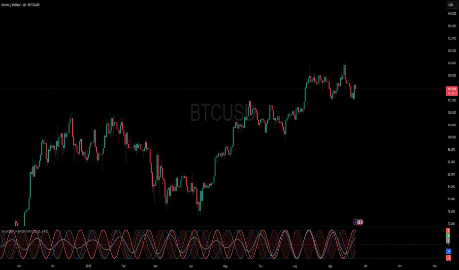
Sinusoidal Cycles OscillatorTitle: Sinusoidal Cycles Oscillator – Multi-Cycle Market Indicator
Description:
Discover market rhythm with the Sinusoidal Cycles Oscillator, a powerful tool for technical analysis and cyclical trading.
Three customizable cycles track short, medium, and long-term market oscillations.
Cycle 1 serves as the main reference wave with an optional mirror envelope.
Cycles 2 & 3 provide supporting harmonics for deeper insight.
Composite wave averages all cycles to reveal overall market phase.
Features:
Fully adjustable periods and amplitude.
Visualize tops, bottoms, and turning points at a glance.
Oscillator ranges from -1 to +1 with clear threshold guides.
Ideal for traders using cycle analysis, harmonic trading, or market timing.
Easy-to-read visual overlay and separate panel option.
Use it to:
Identify potential price reversals.
Compare market cycles across multiple timeframes.
Enhance timing and entry/exit decisions.
在脚本中搜索"harmonic"
Goertzel Cycle Composite Wave [Loxx]As the financial markets become increasingly complex and data-driven, traders and analysts must leverage powerful tools to gain insights and make informed decisions. One such tool is the Goertzel Cycle Composite Wave indicator, a sophisticated technical analysis indicator that helps identify cyclical patterns in financial data. This powerful tool is capable of detecting cyclical patterns in financial data, helping traders to make better predictions and optimize their trading strategies. With its unique combination of mathematical algorithms and advanced charting capabilities, this indicator has the potential to revolutionize the way we approach financial modeling and trading.
*** To decrease the load time of this indicator, only XX many bars back will render to the chart. You can control this value with the setting "Number of Bars to Render". This doesn't have anything to do with repainting or the indicator being endpointed***
█ Brief Overview of the Goertzel Cycle Composite Wave
The Goertzel Cycle Composite Wave is a sophisticated technical analysis tool that utilizes the Goertzel algorithm to analyze and visualize cyclical components within a financial time series. By identifying these cycles and their characteristics, the indicator aims to provide valuable insights into the market's underlying price movements, which could potentially be used for making informed trading decisions.
The Goertzel Cycle Composite Wave is considered a non-repainting and endpointed indicator. This means that once a value has been calculated for a specific bar, that value will not change in subsequent bars, and the indicator is designed to have a clear start and end point. This is an important characteristic for indicators used in technical analysis, as it allows traders to make informed decisions based on historical data without the risk of hindsight bias or future changes in the indicator's values. This means traders can use this indicator trading purposes.
The repainting version of this indicator with forecasting, cycle selection/elimination options, and data output table can be found here:
Goertzel Browser
The primary purpose of this indicator is to:
1. Detect and analyze the dominant cycles present in the price data.
2. Reconstruct and visualize the composite wave based on the detected cycles.
To achieve this, the indicator performs several tasks:
1. Detrending the price data: The indicator preprocesses the price data using various detrending techniques, such as Hodrick-Prescott filters, zero-lag moving averages, and linear regression, to remove the underlying trend and focus on the cyclical components.
2. Applying the Goertzel algorithm: The indicator applies the Goertzel algorithm to the detrended price data, identifying the dominant cycles and their characteristics, such as amplitude, phase, and cycle strength.
3. Constructing the composite wave: The indicator reconstructs the composite wave by combining the detected cycles, either by using a user-defined list of cycles or by selecting the top N cycles based on their amplitude or cycle strength.
4. Visualizing the composite wave: The indicator plots the composite wave, using solid lines for the cycles. The color of the lines indicates whether the wave is increasing or decreasing.
This indicator is a powerful tool that employs the Goertzel algorithm to analyze and visualize the cyclical components within a financial time series. By providing insights into the underlying price movements, the indicator aims to assist traders in making more informed decisions.
█ What is the Goertzel Algorithm?
The Goertzel algorithm, named after Gerald Goertzel, is a digital signal processing technique that is used to efficiently compute individual terms of the Discrete Fourier Transform (DFT). It was first introduced in 1958, and since then, it has found various applications in the fields of engineering, mathematics, and physics.
The Goertzel algorithm is primarily used to detect specific frequency components within a digital signal, making it particularly useful in applications where only a few frequency components are of interest. The algorithm is computationally efficient, as it requires fewer calculations than the Fast Fourier Transform (FFT) when detecting a small number of frequency components. This efficiency makes the Goertzel algorithm a popular choice in applications such as:
1. Telecommunications: The Goertzel algorithm is used for decoding Dual-Tone Multi-Frequency (DTMF) signals, which are the tones generated when pressing buttons on a telephone keypad. By identifying specific frequency components, the algorithm can accurately determine which button has been pressed.
2. Audio processing: The algorithm can be used to detect specific pitches or harmonics in an audio signal, making it useful in applications like pitch detection and tuning musical instruments.
3. Vibration analysis: In the field of mechanical engineering, the Goertzel algorithm can be applied to analyze vibrations in rotating machinery, helping to identify faulty components or signs of wear.
4. Power system analysis: The algorithm can be used to measure harmonic content in power systems, allowing engineers to assess power quality and detect potential issues.
The Goertzel algorithm is used in these applications because it offers several advantages over other methods, such as the FFT:
1. Computational efficiency: The Goertzel algorithm requires fewer calculations when detecting a small number of frequency components, making it more computationally efficient than the FFT in these cases.
2. Real-time analysis: The algorithm can be implemented in a streaming fashion, allowing for real-time analysis of signals, which is crucial in applications like telecommunications and audio processing.
3. Memory efficiency: The Goertzel algorithm requires less memory than the FFT, as it only computes the frequency components of interest.
4. Precision: The algorithm is less susceptible to numerical errors compared to the FFT, ensuring more accurate results in applications where precision is essential.
The Goertzel algorithm is an efficient digital signal processing technique that is primarily used to detect specific frequency components within a signal. Its computational efficiency, real-time capabilities, and precision make it an attractive choice for various applications, including telecommunications, audio processing, vibration analysis, and power system analysis. The algorithm has been widely adopted since its introduction in 1958 and continues to be an essential tool in the fields of engineering, mathematics, and physics.
█ Goertzel Algorithm in Quantitative Finance: In-Depth Analysis and Applications
The Goertzel algorithm, initially designed for signal processing in telecommunications, has gained significant traction in the financial industry due to its efficient frequency detection capabilities. In quantitative finance, the Goertzel algorithm has been utilized for uncovering hidden market cycles, developing data-driven trading strategies, and optimizing risk management. This section delves deeper into the applications of the Goertzel algorithm in finance, particularly within the context of quantitative trading and analysis.
Unveiling Hidden Market Cycles:
Market cycles are prevalent in financial markets and arise from various factors, such as economic conditions, investor psychology, and market participant behavior. The Goertzel algorithm's ability to detect and isolate specific frequencies in price data helps trader analysts identify hidden market cycles that may otherwise go unnoticed. By examining the amplitude, phase, and periodicity of each cycle, traders can better understand the underlying market structure and dynamics, enabling them to develop more informed and effective trading strategies.
Developing Quantitative Trading Strategies:
The Goertzel algorithm's versatility allows traders to incorporate its insights into a wide range of trading strategies. By identifying the dominant market cycles in a financial instrument's price data, traders can create data-driven strategies that capitalize on the cyclical nature of markets.
For instance, a trader may develop a mean-reversion strategy that takes advantage of the identified cycles. By establishing positions when the price deviates from the predicted cycle, the trader can profit from the subsequent reversion to the cycle's mean. Similarly, a momentum-based strategy could be designed to exploit the persistence of a dominant cycle by entering positions that align with the cycle's direction.
Enhancing Risk Management:
The Goertzel algorithm plays a vital role in risk management for quantitative strategies. By analyzing the cyclical components of a financial instrument's price data, traders can gain insights into the potential risks associated with their trading strategies.
By monitoring the amplitude and phase of dominant cycles, a trader can detect changes in market dynamics that may pose risks to their positions. For example, a sudden increase in amplitude may indicate heightened volatility, prompting the trader to adjust position sizing or employ hedging techniques to protect their portfolio. Additionally, changes in phase alignment could signal a potential shift in market sentiment, necessitating adjustments to the trading strategy.
Expanding Quantitative Toolkits:
Traders can augment the Goertzel algorithm's insights by combining it with other quantitative techniques, creating a more comprehensive and sophisticated analysis framework. For example, machine learning algorithms, such as neural networks or support vector machines, could be trained on features extracted from the Goertzel algorithm to predict future price movements more accurately.
Furthermore, the Goertzel algorithm can be integrated with other technical analysis tools, such as moving averages or oscillators, to enhance their effectiveness. By applying these tools to the identified cycles, traders can generate more robust and reliable trading signals.
The Goertzel algorithm offers invaluable benefits to quantitative finance practitioners by uncovering hidden market cycles, aiding in the development of data-driven trading strategies, and improving risk management. By leveraging the insights provided by the Goertzel algorithm and integrating it with other quantitative techniques, traders can gain a deeper understanding of market dynamics and devise more effective trading strategies.
█ Indicator Inputs
src: This is the source data for the analysis, typically the closing price of the financial instrument.
detrendornot: This input determines the method used for detrending the source data. Detrending is the process of removing the underlying trend from the data to focus on the cyclical components.
The available options are:
hpsmthdt: Detrend using Hodrick-Prescott filter centered moving average.
zlagsmthdt: Detrend using zero-lag moving average centered moving average.
logZlagRegression: Detrend using logarithmic zero-lag linear regression.
hpsmth: Detrend using Hodrick-Prescott filter.
zlagsmth: Detrend using zero-lag moving average.
DT_HPper1 and DT_HPper2: These inputs define the period range for the Hodrick-Prescott filter centered moving average when detrendornot is set to hpsmthdt.
DT_ZLper1 and DT_ZLper2: These inputs define the period range for the zero-lag moving average centered moving average when detrendornot is set to zlagsmthdt.
DT_RegZLsmoothPer: This input defines the period for the zero-lag moving average used in logarithmic zero-lag linear regression when detrendornot is set to logZlagRegression.
HPsmoothPer: This input defines the period for the Hodrick-Prescott filter when detrendornot is set to hpsmth.
ZLMAsmoothPer: This input defines the period for the zero-lag moving average when detrendornot is set to zlagsmth.
MaxPer: This input sets the maximum period for the Goertzel algorithm to search for cycles.
squaredAmp: This boolean input determines whether the amplitude should be squared in the Goertzel algorithm.
useAddition: This boolean input determines whether the Goertzel algorithm should use addition for combining the cycles.
useCosine: This boolean input determines whether the Goertzel algorithm should use cosine waves instead of sine waves.
UseCycleStrength: This boolean input determines whether the Goertzel algorithm should compute the cycle strength, which is a normalized measure of the cycle's amplitude.
WindowSizePast: These inputs define the window size for the composite wave.
FilterBartels: This boolean input determines whether Bartel's test should be applied to filter out non-significant cycles.
BartNoCycles: This input sets the number of cycles to be used in Bartel's test.
BartSmoothPer: This input sets the period for the moving average used in Bartel's test.
BartSigLimit: This input sets the significance limit for Bartel's test, below which cycles are considered insignificant.
SortBartels: This boolean input determines whether the cycles should be sorted by their Bartel's test results.
StartAtCycle: This input determines the starting index for selecting the top N cycles when UseCycleList is set to false. This allows you to skip a certain number of cycles from the top before selecting the desired number of cycles.
UseTopCycles: This input sets the number of top cycles to use for constructing the composite wave when UseCycleList is set to false. The cycles are ranked based on their amplitudes or cycle strengths, depending on the UseCycleStrength input.
SubtractNoise: This boolean input determines whether to subtract the noise (remaining cycles) from the composite wave. If set to true, the composite wave will only include the top N cycles specified by UseTopCycles.
█ Exploring Auxiliary Functions
The following functions demonstrate advanced techniques for analyzing financial markets, including zero-lag moving averages, Bartels probability, detrending, and Hodrick-Prescott filtering. This section examines each function in detail, explaining their purpose, methodology, and applications in finance. We will examine how each function contributes to the overall performance and effectiveness of the indicator and how they work together to create a powerful analytical tool.
Zero-Lag Moving Average:
The zero-lag moving average function is designed to minimize the lag typically associated with moving averages. This is achieved through a two-step weighted linear regression process that emphasizes more recent data points. The function calculates a linearly weighted moving average (LWMA) on the input data and then applies another LWMA on the result. By doing this, the function creates a moving average that closely follows the price action, reducing the lag and improving the responsiveness of the indicator.
The zero-lag moving average function is used in the indicator to provide a responsive, low-lag smoothing of the input data. This function helps reduce the noise and fluctuations in the data, making it easier to identify and analyze underlying trends and patterns. By minimizing the lag associated with traditional moving averages, this function allows the indicator to react more quickly to changes in market conditions, providing timely signals and improving the overall effectiveness of the indicator.
Bartels Probability:
The Bartels probability function calculates the probability of a given cycle being significant in a time series. It uses a mathematical test called the Bartels test to assess the significance of cycles detected in the data. The function calculates coefficients for each detected cycle and computes an average amplitude and an expected amplitude. By comparing these values, the Bartels probability is derived, indicating the likelihood of a cycle's significance. This information can help in identifying and analyzing dominant cycles in financial markets.
The Bartels probability function is incorporated into the indicator to assess the significance of detected cycles in the input data. By calculating the Bartels probability for each cycle, the indicator can prioritize the most significant cycles and focus on the market dynamics that are most relevant to the current trading environment. This function enhances the indicator's ability to identify dominant market cycles, improving its predictive power and aiding in the development of effective trading strategies.
Detrend Logarithmic Zero-Lag Regression:
The detrend logarithmic zero-lag regression function is used for detrending data while minimizing lag. It combines a zero-lag moving average with a linear regression detrending method. The function first calculates the zero-lag moving average of the logarithm of input data and then applies a linear regression to remove the trend. By detrending the data, the function isolates the cyclical components, making it easier to analyze and interpret the underlying market dynamics.
The detrend logarithmic zero-lag regression function is used in the indicator to isolate the cyclical components of the input data. By detrending the data, the function enables the indicator to focus on the cyclical movements in the market, making it easier to analyze and interpret market dynamics. This function is essential for identifying cyclical patterns and understanding the interactions between different market cycles, which can inform trading decisions and enhance overall market understanding.
Bartels Cycle Significance Test:
The Bartels cycle significance test is a function that combines the Bartels probability function and the detrend logarithmic zero-lag regression function to assess the significance of detected cycles. The function calculates the Bartels probability for each cycle and stores the results in an array. By analyzing the probability values, traders and analysts can identify the most significant cycles in the data, which can be used to develop trading strategies and improve market understanding.
The Bartels cycle significance test function is integrated into the indicator to provide a comprehensive analysis of the significance of detected cycles. By combining the Bartels probability function and the detrend logarithmic zero-lag regression function, this test evaluates the significance of each cycle and stores the results in an array. The indicator can then use this information to prioritize the most significant cycles and focus on the most relevant market dynamics. This function enhances the indicator's ability to identify and analyze dominant market cycles, providing valuable insights for trading and market analysis.
Hodrick-Prescott Filter:
The Hodrick-Prescott filter is a popular technique used to separate the trend and cyclical components of a time series. The function applies a smoothing parameter to the input data and calculates a smoothed series using a two-sided filter. This smoothed series represents the trend component, which can be subtracted from the original data to obtain the cyclical component. The Hodrick-Prescott filter is commonly used in economics and finance to analyze economic data and financial market trends.
The Hodrick-Prescott filter is incorporated into the indicator to separate the trend and cyclical components of the input data. By applying the filter to the data, the indicator can isolate the trend component, which can be used to analyze long-term market trends and inform trading decisions. Additionally, the cyclical component can be used to identify shorter-term market dynamics and provide insights into potential trading opportunities. The inclusion of the Hodrick-Prescott filter adds another layer of analysis to the indicator, making it more versatile and comprehensive.
Detrending Options: Detrend Centered Moving Average:
The detrend centered moving average function provides different detrending methods, including the Hodrick-Prescott filter and the zero-lag moving average, based on the selected detrending method. The function calculates two sets of smoothed values using the chosen method and subtracts one set from the other to obtain a detrended series. By offering multiple detrending options, this function allows traders and analysts to select the most appropriate method for their specific needs and preferences.
The detrend centered moving average function is integrated into the indicator to provide users with multiple detrending options, including the Hodrick-Prescott filter and the zero-lag moving average. By offering multiple detrending methods, the indicator allows users to customize the analysis to their specific needs and preferences, enhancing the indicator's overall utility and adaptability. This function ensures that the indicator can cater to a wide range of trading styles and objectives, making it a valuable tool for a diverse group of market participants.
The auxiliary functions functions discussed in this section demonstrate the power and versatility of mathematical techniques in analyzing financial markets. By understanding and implementing these functions, traders and analysts can gain valuable insights into market dynamics, improve their trading strategies, and make more informed decisions. The combination of zero-lag moving averages, Bartels probability, detrending methods, and the Hodrick-Prescott filter provides a comprehensive toolkit for analyzing and interpreting financial data. The integration of advanced functions in a financial indicator creates a powerful and versatile analytical tool that can provide valuable insights into financial markets. By combining the zero-lag moving average,
█ In-Depth Analysis of the Goertzel Cycle Composite Wave Code
The Goertzel Cycle Composite Wave code is an implementation of the Goertzel Algorithm, an efficient technique to perform spectral analysis on a signal. The code is designed to detect and analyze dominant cycles within a given financial market data set. This section will provide an extremely detailed explanation of the code, its structure, functions, and intended purpose.
Function signature and input parameters:
The Goertzel Cycle Composite Wave function accepts numerous input parameters for customization, including source data (src), the current bar (forBar), sample size (samplesize), period (per), squared amplitude flag (squaredAmp), addition flag (useAddition), cosine flag (useCosine), cycle strength flag (UseCycleStrength), past sizes (WindowSizePast), Bartels filter flag (FilterBartels), Bartels-related parameters (BartNoCycles, BartSmoothPer, BartSigLimit), sorting flag (SortBartels), and output buffers (goeWorkPast, cyclebuffer, amplitudebuffer, phasebuffer, cycleBartelsBuffer).
Initializing variables and arrays:
The code initializes several float arrays (goeWork1, goeWork2, goeWork3, goeWork4) with the same length as twice the period (2 * per). These arrays store intermediate results during the execution of the algorithm.
Preprocessing input data:
The input data (src) undergoes preprocessing to remove linear trends. This step enhances the algorithm's ability to focus on cyclical components in the data. The linear trend is calculated by finding the slope between the first and last values of the input data within the sample.
Iterative calculation of Goertzel coefficients:
The core of the Goertzel Cycle Composite Wave algorithm lies in the iterative calculation of Goertzel coefficients for each frequency bin. These coefficients represent the spectral content of the input data at different frequencies. The code iterates through the range of frequencies, calculating the Goertzel coefficients using a nested loop structure.
Cycle strength computation:
The code calculates the cycle strength based on the Goertzel coefficients. This is an optional step, controlled by the UseCycleStrength flag. The cycle strength provides information on the relative influence of each cycle on the data per bar, considering both amplitude and cycle length. The algorithm computes the cycle strength either by squaring the amplitude (controlled by squaredAmp flag) or using the actual amplitude values.
Phase calculation:
The Goertzel Cycle Composite Wave code computes the phase of each cycle, which represents the position of the cycle within the input data. The phase is calculated using the arctangent function (math.atan) based on the ratio of the imaginary and real components of the Goertzel coefficients.
Peak detection and cycle extraction:
The algorithm performs peak detection on the computed amplitudes or cycle strengths to identify dominant cycles. It stores the detected cycles in the cyclebuffer array, along with their corresponding amplitudes and phases in the amplitudebuffer and phasebuffer arrays, respectively.
Sorting cycles by amplitude or cycle strength:
The code sorts the detected cycles based on their amplitude or cycle strength in descending order. This allows the algorithm to prioritize cycles with the most significant impact on the input data.
Bartels cycle significance test:
If the FilterBartels flag is set, the code performs a Bartels cycle significance test on the detected cycles. This test determines the statistical significance of each cycle and filters out the insignificant cycles. The significant cycles are stored in the cycleBartelsBuffer array. If the SortBartels flag is set, the code sorts the significant cycles based on their Bartels significance values.
Waveform calculation:
The Goertzel Cycle Composite Wave code calculates the waveform of the significant cycles for specified time windows. The windows are defined by the WindowSizePast parameters, respectively. The algorithm uses either cosine or sine functions (controlled by the useCosine flag) to calculate the waveforms for each cycle. The useAddition flag determines whether the waveforms should be added or subtracted.
Storing waveforms in a matrix:
The calculated waveforms for the cycle is stored in the matrix - goeWorkPast. This matrix holds the waveforms for the specified time windows. Each row in the matrix represents a time window position, and each column corresponds to a cycle.
Returning the number of cycles:
The Goertzel Cycle Composite Wave function returns the total number of detected cycles (number_of_cycles) after processing the input data. This information can be used to further analyze the results or to visualize the detected cycles.
The Goertzel Cycle Composite Wave code is a comprehensive implementation of the Goertzel Algorithm, specifically designed for detecting and analyzing dominant cycles within financial market data. The code offers a high level of customization, allowing users to fine-tune the algorithm based on their specific needs. The Goertzel Cycle Composite Wave's combination of preprocessing, iterative calculations, cycle extraction, sorting, significance testing, and waveform calculation makes it a powerful tool for understanding cyclical components in financial data.
█ Generating and Visualizing Composite Waveform
The indicator calculates and visualizes the composite waveform for specified time windows based on the detected cycles. Here's a detailed explanation of this process:
Updating WindowSizePast:
The WindowSizePast is updated to ensure they are at least twice the MaxPer (maximum period).
Initializing matrices and arrays:
The matrix goeWorkPast is initialized to store the Goertzel results for specified time windows. Multiple arrays are also initialized to store cycle, amplitude, phase, and Bartels information.
Preparing the source data (srcVal) array:
The source data is copied into an array, srcVal, and detrended using one of the selected methods (hpsmthdt, zlagsmthdt, logZlagRegression, hpsmth, or zlagsmth).
Goertzel function call:
The Goertzel function is called to analyze the detrended source data and extract cycle information. The output, number_of_cycles, contains the number of detected cycles.
Initializing arrays for waveforms:
The goertzel array is initialized to store the endpoint Goertzel.
Calculating composite waveform (goertzel array):
The composite waveform is calculated by summing the selected cycles (either from the user-defined cycle list or the top cycles) and optionally subtracting the noise component.
Drawing composite waveform (pvlines):
The composite waveform is drawn on the chart using solid lines. The color of the lines is determined by the direction of the waveform (green for upward, red for downward).
To summarize, this indicator generates a composite waveform based on the detected cycles in the financial data. It calculates the composite waveforms and visualizes them on the chart using colored lines.
█ Enhancing the Goertzel Algorithm-Based Script for Financial Modeling and Trading
The Goertzel algorithm-based script for detecting dominant cycles in financial data is a powerful tool for financial modeling and trading. It provides valuable insights into the past behavior of these cycles. However, as with any algorithm, there is always room for improvement. This section discusses potential enhancements to the existing script to make it even more robust and versatile for financial modeling, general trading, advanced trading, and high-frequency finance trading.
Enhancements for Financial Modeling
Data preprocessing: One way to improve the script's performance for financial modeling is to introduce more advanced data preprocessing techniques. This could include removing outliers, handling missing data, and normalizing the data to ensure consistent and accurate results.
Additional detrending and smoothing methods: Incorporating more sophisticated detrending and smoothing techniques, such as wavelet transform or empirical mode decomposition, can help improve the script's ability to accurately identify cycles and trends in the data.
Machine learning integration: Integrating machine learning techniques, such as artificial neural networks or support vector machines, can help enhance the script's predictive capabilities, leading to more accurate financial models.
Enhancements for General and Advanced Trading
Customizable indicator integration: Allowing users to integrate their own technical indicators can help improve the script's effectiveness for both general and advanced trading. By enabling the combination of the dominant cycle information with other technical analysis tools, traders can develop more comprehensive trading strategies.
Risk management and position sizing: Incorporating risk management and position sizing functionality into the script can help traders better manage their trades and control potential losses. This can be achieved by calculating the optimal position size based on the user's risk tolerance and account size.
Multi-timeframe analysis: Enhancing the script to perform multi-timeframe analysis can provide traders with a more holistic view of market trends and cycles. By identifying dominant cycles on different timeframes, traders can gain insights into the potential confluence of cycles and make better-informed trading decisions.
Enhancements for High-Frequency Finance Trading
Algorithm optimization: To ensure the script's suitability for high-frequency finance trading, optimizing the algorithm for faster execution is crucial. This can be achieved by employing efficient data structures and refining the calculation methods to minimize computational complexity.
Real-time data streaming: Integrating real-time data streaming capabilities into the script can help high-frequency traders react to market changes more quickly. By continuously updating the cycle information based on real-time market data, traders can adapt their strategies accordingly and capitalize on short-term market fluctuations.
Order execution and trade management: To fully leverage the script's capabilities for high-frequency trading, implementing functionality for automated order execution and trade management is essential. This can include features such as stop-loss and take-profit orders, trailing stops, and automated trade exit strategies.
While the existing Goertzel algorithm-based script is a valuable tool for detecting dominant cycles in financial data, there are several potential enhancements that can make it even more powerful for financial modeling, general trading, advanced trading, and high-frequency finance trading. By incorporating these improvements, the script can become a more versatile and effective tool for traders and financial analysts alike.
█ Understanding the Limitations of the Goertzel Algorithm
While the Goertzel algorithm-based script for detecting dominant cycles in financial data provides valuable insights, it is important to be aware of its limitations and drawbacks. Some of the key drawbacks of this indicator are:
Lagging nature:
As with many other technical indicators, the Goertzel algorithm-based script can suffer from lagging effects, meaning that it may not immediately react to real-time market changes. This lag can lead to late entries and exits, potentially resulting in reduced profitability or increased losses.
Parameter sensitivity:
The performance of the script can be sensitive to the chosen parameters, such as the detrending methods, smoothing techniques, and cycle detection settings. Improper parameter selection may lead to inaccurate cycle detection or increased false signals, which can negatively impact trading performance.
Complexity:
The Goertzel algorithm itself is relatively complex, making it difficult for novice traders or those unfamiliar with the concept of cycle analysis to fully understand and effectively utilize the script. This complexity can also make it challenging to optimize the script for specific trading styles or market conditions.
Overfitting risk:
As with any data-driven approach, there is a risk of overfitting when using the Goertzel algorithm-based script. Overfitting occurs when a model becomes too specific to the historical data it was trained on, leading to poor performance on new, unseen data. This can result in misleading signals and reduced trading performance.
Limited applicability:
The Goertzel algorithm-based script may not be suitable for all markets, trading styles, or timeframes. Its effectiveness in detecting cycles may be limited in certain market conditions, such as during periods of extreme volatility or low liquidity.
While the Goertzel algorithm-based script offers valuable insights into dominant cycles in financial data, it is essential to consider its drawbacks and limitations when incorporating it into a trading strategy. Traders should always use the script in conjunction with other technical and fundamental analysis tools, as well as proper risk management, to make well-informed trading decisions.
█ Interpreting Results
The Goertzel Cycle Composite Wave indicator can be interpreted by analyzing the plotted lines. The indicator plots two lines: composite waves. The composite wave represents the composite wave of the price data.
The composite wave line displays a solid line, with green indicating a bullish trend and red indicating a bearish trend.
Interpreting the Goertzel Cycle Composite Wave indicator involves identifying the trend of the composite wave lines and matching them with the corresponding bullish or bearish color.
█ Conclusion
The Goertzel Cycle Composite Wave indicator is a powerful tool for identifying and analyzing cyclical patterns in financial markets. Its ability to detect multiple cycles of varying frequencies and strengths make it a valuable addition to any trader's technical analysis toolkit. However, it is important to keep in mind that the Goertzel Cycle Composite Wave indicator should be used in conjunction with other technical analysis tools and fundamental analysis to achieve the best results. With continued refinement and development, the Goertzel Cycle Composite Wave indicator has the potential to become a highly effective tool for financial modeling, general trading, advanced trading, and high-frequency finance trading. Its accuracy and versatility make it a promising candidate for further research and development.
█ Footnotes
What is the Bartels Test for Cycle Significance?
The Bartels Cycle Significance Test is a statistical method that determines whether the peaks and troughs of a time series are statistically significant. The test is named after its inventor, George Bartels, who developed it in the mid-20th century.
The Bartels test is designed to analyze the cyclical components of a time series, which can help traders and analysts identify trends and cycles in financial markets. The test calculates a Bartels statistic, which measures the degree of non-randomness or autocorrelation in the time series.
The Bartels statistic is calculated by first splitting the time series into two halves and calculating the range of the peaks and troughs in each half. The test then compares these ranges using a t-test, which measures the significance of the difference between the two ranges.
If the Bartels statistic is greater than a critical value, it indicates that the peaks and troughs in the time series are non-random and that there is a significant cyclical component to the data. Conversely, if the Bartels statistic is less than the critical value, it suggests that the peaks and troughs are random and that there is no significant cyclical component.
The Bartels Cycle Significance Test is particularly useful in financial analysis because it can help traders and analysts identify significant cycles in asset prices, which can in turn inform investment decisions. However, it is important to note that the test is not perfect and can produce false signals in certain situations, particularly in noisy or volatile markets. Therefore, it is always recommended to use the test in conjunction with other technical and fundamental indicators to confirm trends and cycles.
Deep-dive into the Hodrick-Prescott Fitler
The Hodrick-Prescott (HP) filter is a statistical tool used in economics and finance to separate a time series into two components: a trend component and a cyclical component. It is a powerful tool for identifying long-term trends in economic and financial data and is widely used by economists, central banks, and financial institutions around the world.
The HP filter was first introduced in the 1990s by economists Robert Hodrick and Edward Prescott. It is a simple, two-parameter filter that separates a time series into a trend component and a cyclical component. The trend component represents the long-term behavior of the data, while the cyclical component captures the shorter-term fluctuations around the trend.
The HP filter works by minimizing the following objective function:
Minimize: (Sum of Squared Deviations) + λ (Sum of Squared Second Differences)
Where:
1. The first term represents the deviation of the data from the trend.
2. The second term represents the smoothness of the trend.
3. λ is a smoothing parameter that determines the degree of smoothness of the trend.
The smoothing parameter λ is typically set to a value between 100 and 1600, depending on the frequency of the data. Higher values of λ lead to a smoother trend, while lower values lead to a more volatile trend.
The HP filter has several advantages over other smoothing techniques. It is a non-parametric method, meaning that it does not make any assumptions about the underlying distribution of the data. It also allows for easy comparison of trends across different time series and can be used with data of any frequency.
However, the HP filter also has some limitations. It assumes that the trend is a smooth function, which may not be the case in some situations. It can also be sensitive to changes in the smoothing parameter λ, which may result in different trends for the same data. Additionally, the filter may produce unrealistic trends for very short time series.
Despite these limitations, the HP filter remains a valuable tool for analyzing economic and financial data. It is widely used by central banks and financial institutions to monitor long-term trends in the economy, and it can be used to identify turning points in the business cycle. The filter can also be used to analyze asset prices, exchange rates, and other financial variables.
The Hodrick-Prescott filter is a powerful tool for analyzing economic and financial data. It separates a time series into a trend component and a cyclical component, allowing for easy identification of long-term trends and turning points in the business cycle. While it has some limitations, it remains a valuable tool for economists, central banks, and financial institutions around the world.

Goertzel Browser [Loxx]As the financial markets become increasingly complex and data-driven, traders and analysts must leverage powerful tools to gain insights and make informed decisions. One such tool is the Goertzel Browser indicator, a sophisticated technical analysis indicator that helps identify cyclical patterns in financial data. This powerful tool is capable of detecting cyclical patterns in financial data, helping traders to make better predictions and optimize their trading strategies. With its unique combination of mathematical algorithms and advanced charting capabilities, this indicator has the potential to revolutionize the way we approach financial modeling and trading.
█ Brief Overview of the Goertzel Browser
The Goertzel Browser is a sophisticated technical analysis tool that utilizes the Goertzel algorithm to analyze and visualize cyclical components within a financial time series. By identifying these cycles and their characteristics, the indicator aims to provide valuable insights into the market's underlying price movements, which could potentially be used for making informed trading decisions.
The primary purpose of this indicator is to:
1. Detect and analyze the dominant cycles present in the price data.
2. Reconstruct and visualize the composite wave based on the detected cycles.
3. Project the composite wave into the future, providing a potential roadmap for upcoming price movements.
To achieve this, the indicator performs several tasks:
1. Detrending the price data: The indicator preprocesses the price data using various detrending techniques, such as Hodrick-Prescott filters, zero-lag moving averages, and linear regression, to remove the underlying trend and focus on the cyclical components.
2. Applying the Goertzel algorithm: The indicator applies the Goertzel algorithm to the detrended price data, identifying the dominant cycles and their characteristics, such as amplitude, phase, and cycle strength.
3. Constructing the composite wave: The indicator reconstructs the composite wave by combining the detected cycles, either by using a user-defined list of cycles or by selecting the top N cycles based on their amplitude or cycle strength.
4. Visualizing the composite wave: The indicator plots the composite wave, using solid lines for the past and dotted lines for the future projections. The color of the lines indicates whether the wave is increasing or decreasing.
5. Displaying cycle information: The indicator provides a table that displays detailed information about the detected cycles, including their rank, period, Bartel's test results, amplitude, and phase.
This indicator is a powerful tool that employs the Goertzel algorithm to analyze and visualize the cyclical components within a financial time series. By providing insights into the underlying price movements and their potential future trajectory, the indicator aims to assist traders in making more informed decisions.
█ What is the Goertzel Algorithm?
The Goertzel algorithm, named after Gerald Goertzel, is a digital signal processing technique that is used to efficiently compute individual terms of the Discrete Fourier Transform (DFT). It was first introduced in 1958, and since then, it has found various applications in the fields of engineering, mathematics, and physics.
The Goertzel algorithm is primarily used to detect specific frequency components within a digital signal, making it particularly useful in applications where only a few frequency components are of interest. The algorithm is computationally efficient, as it requires fewer calculations than the Fast Fourier Transform (FFT) when detecting a small number of frequency components. This efficiency makes the Goertzel algorithm a popular choice in applications such as:
1. Telecommunications: The Goertzel algorithm is used for decoding Dual-Tone Multi-Frequency (DTMF) signals, which are the tones generated when pressing buttons on a telephone keypad. By identifying specific frequency components, the algorithm can accurately determine which button has been pressed.
2. Audio processing: The algorithm can be used to detect specific pitches or harmonics in an audio signal, making it useful in applications like pitch detection and tuning musical instruments.
3. Vibration analysis: In the field of mechanical engineering, the Goertzel algorithm can be applied to analyze vibrations in rotating machinery, helping to identify faulty components or signs of wear.
4. Power system analysis: The algorithm can be used to measure harmonic content in power systems, allowing engineers to assess power quality and detect potential issues.
The Goertzel algorithm is used in these applications because it offers several advantages over other methods, such as the FFT:
1. Computational efficiency: The Goertzel algorithm requires fewer calculations when detecting a small number of frequency components, making it more computationally efficient than the FFT in these cases.
2. Real-time analysis: The algorithm can be implemented in a streaming fashion, allowing for real-time analysis of signals, which is crucial in applications like telecommunications and audio processing.
3. Memory efficiency: The Goertzel algorithm requires less memory than the FFT, as it only computes the frequency components of interest.
4. Precision: The algorithm is less susceptible to numerical errors compared to the FFT, ensuring more accurate results in applications where precision is essential.
The Goertzel algorithm is an efficient digital signal processing technique that is primarily used to detect specific frequency components within a signal. Its computational efficiency, real-time capabilities, and precision make it an attractive choice for various applications, including telecommunications, audio processing, vibration analysis, and power system analysis. The algorithm has been widely adopted since its introduction in 1958 and continues to be an essential tool in the fields of engineering, mathematics, and physics.
█ Goertzel Algorithm in Quantitative Finance: In-Depth Analysis and Applications
The Goertzel algorithm, initially designed for signal processing in telecommunications, has gained significant traction in the financial industry due to its efficient frequency detection capabilities. In quantitative finance, the Goertzel algorithm has been utilized for uncovering hidden market cycles, developing data-driven trading strategies, and optimizing risk management. This section delves deeper into the applications of the Goertzel algorithm in finance, particularly within the context of quantitative trading and analysis.
Unveiling Hidden Market Cycles:
Market cycles are prevalent in financial markets and arise from various factors, such as economic conditions, investor psychology, and market participant behavior. The Goertzel algorithm's ability to detect and isolate specific frequencies in price data helps trader analysts identify hidden market cycles that may otherwise go unnoticed. By examining the amplitude, phase, and periodicity of each cycle, traders can better understand the underlying market structure and dynamics, enabling them to develop more informed and effective trading strategies.
Developing Quantitative Trading Strategies:
The Goertzel algorithm's versatility allows traders to incorporate its insights into a wide range of trading strategies. By identifying the dominant market cycles in a financial instrument's price data, traders can create data-driven strategies that capitalize on the cyclical nature of markets.
For instance, a trader may develop a mean-reversion strategy that takes advantage of the identified cycles. By establishing positions when the price deviates from the predicted cycle, the trader can profit from the subsequent reversion to the cycle's mean. Similarly, a momentum-based strategy could be designed to exploit the persistence of a dominant cycle by entering positions that align with the cycle's direction.
Enhancing Risk Management:
The Goertzel algorithm plays a vital role in risk management for quantitative strategies. By analyzing the cyclical components of a financial instrument's price data, traders can gain insights into the potential risks associated with their trading strategies.
By monitoring the amplitude and phase of dominant cycles, a trader can detect changes in market dynamics that may pose risks to their positions. For example, a sudden increase in amplitude may indicate heightened volatility, prompting the trader to adjust position sizing or employ hedging techniques to protect their portfolio. Additionally, changes in phase alignment could signal a potential shift in market sentiment, necessitating adjustments to the trading strategy.
Expanding Quantitative Toolkits:
Traders can augment the Goertzel algorithm's insights by combining it with other quantitative techniques, creating a more comprehensive and sophisticated analysis framework. For example, machine learning algorithms, such as neural networks or support vector machines, could be trained on features extracted from the Goertzel algorithm to predict future price movements more accurately.
Furthermore, the Goertzel algorithm can be integrated with other technical analysis tools, such as moving averages or oscillators, to enhance their effectiveness. By applying these tools to the identified cycles, traders can generate more robust and reliable trading signals.
The Goertzel algorithm offers invaluable benefits to quantitative finance practitioners by uncovering hidden market cycles, aiding in the development of data-driven trading strategies, and improving risk management. By leveraging the insights provided by the Goertzel algorithm and integrating it with other quantitative techniques, traders can gain a deeper understanding of market dynamics and devise more effective trading strategies.
█ Indicator Inputs
src: This is the source data for the analysis, typically the closing price of the financial instrument.
detrendornot: This input determines the method used for detrending the source data. Detrending is the process of removing the underlying trend from the data to focus on the cyclical components.
The available options are:
hpsmthdt: Detrend using Hodrick-Prescott filter centered moving average.
zlagsmthdt: Detrend using zero-lag moving average centered moving average.
logZlagRegression: Detrend using logarithmic zero-lag linear regression.
hpsmth: Detrend using Hodrick-Prescott filter.
zlagsmth: Detrend using zero-lag moving average.
DT_HPper1 and DT_HPper2: These inputs define the period range for the Hodrick-Prescott filter centered moving average when detrendornot is set to hpsmthdt.
DT_ZLper1 and DT_ZLper2: These inputs define the period range for the zero-lag moving average centered moving average when detrendornot is set to zlagsmthdt.
DT_RegZLsmoothPer: This input defines the period for the zero-lag moving average used in logarithmic zero-lag linear regression when detrendornot is set to logZlagRegression.
HPsmoothPer: This input defines the period for the Hodrick-Prescott filter when detrendornot is set to hpsmth.
ZLMAsmoothPer: This input defines the period for the zero-lag moving average when detrendornot is set to zlagsmth.
MaxPer: This input sets the maximum period for the Goertzel algorithm to search for cycles.
squaredAmp: This boolean input determines whether the amplitude should be squared in the Goertzel algorithm.
useAddition: This boolean input determines whether the Goertzel algorithm should use addition for combining the cycles.
useCosine: This boolean input determines whether the Goertzel algorithm should use cosine waves instead of sine waves.
UseCycleStrength: This boolean input determines whether the Goertzel algorithm should compute the cycle strength, which is a normalized measure of the cycle's amplitude.
WindowSizePast and WindowSizeFuture: These inputs define the window size for past and future projections of the composite wave.
FilterBartels: This boolean input determines whether Bartel's test should be applied to filter out non-significant cycles.
BartNoCycles: This input sets the number of cycles to be used in Bartel's test.
BartSmoothPer: This input sets the period for the moving average used in Bartel's test.
BartSigLimit: This input sets the significance limit for Bartel's test, below which cycles are considered insignificant.
SortBartels: This boolean input determines whether the cycles should be sorted by their Bartel's test results.
UseCycleList: This boolean input determines whether a user-defined list of cycles should be used for constructing the composite wave. If set to false, the top N cycles will be used.
Cycle1, Cycle2, Cycle3, Cycle4, and Cycle5: These inputs define the user-defined list of cycles when 'UseCycleList' is set to true. If using a user-defined list, each of these inputs represents the period of a specific cycle to include in the composite wave.
StartAtCycle: This input determines the starting index for selecting the top N cycles when UseCycleList is set to false. This allows you to skip a certain number of cycles from the top before selecting the desired number of cycles.
UseTopCycles: This input sets the number of top cycles to use for constructing the composite wave when UseCycleList is set to false. The cycles are ranked based on their amplitudes or cycle strengths, depending on the UseCycleStrength input.
SubtractNoise: This boolean input determines whether to subtract the noise (remaining cycles) from the composite wave. If set to true, the composite wave will only include the top N cycles specified by UseTopCycles.
█ Exploring Auxiliary Functions
The following functions demonstrate advanced techniques for analyzing financial markets, including zero-lag moving averages, Bartels probability, detrending, and Hodrick-Prescott filtering. This section examines each function in detail, explaining their purpose, methodology, and applications in finance. We will examine how each function contributes to the overall performance and effectiveness of the indicator and how they work together to create a powerful analytical tool.
Zero-Lag Moving Average:
The zero-lag moving average function is designed to minimize the lag typically associated with moving averages. This is achieved through a two-step weighted linear regression process that emphasizes more recent data points. The function calculates a linearly weighted moving average (LWMA) on the input data and then applies another LWMA on the result. By doing this, the function creates a moving average that closely follows the price action, reducing the lag and improving the responsiveness of the indicator.
The zero-lag moving average function is used in the indicator to provide a responsive, low-lag smoothing of the input data. This function helps reduce the noise and fluctuations in the data, making it easier to identify and analyze underlying trends and patterns. By minimizing the lag associated with traditional moving averages, this function allows the indicator to react more quickly to changes in market conditions, providing timely signals and improving the overall effectiveness of the indicator.
Bartels Probability:
The Bartels probability function calculates the probability of a given cycle being significant in a time series. It uses a mathematical test called the Bartels test to assess the significance of cycles detected in the data. The function calculates coefficients for each detected cycle and computes an average amplitude and an expected amplitude. By comparing these values, the Bartels probability is derived, indicating the likelihood of a cycle's significance. This information can help in identifying and analyzing dominant cycles in financial markets.
The Bartels probability function is incorporated into the indicator to assess the significance of detected cycles in the input data. By calculating the Bartels probability for each cycle, the indicator can prioritize the most significant cycles and focus on the market dynamics that are most relevant to the current trading environment. This function enhances the indicator's ability to identify dominant market cycles, improving its predictive power and aiding in the development of effective trading strategies.
Detrend Logarithmic Zero-Lag Regression:
The detrend logarithmic zero-lag regression function is used for detrending data while minimizing lag. It combines a zero-lag moving average with a linear regression detrending method. The function first calculates the zero-lag moving average of the logarithm of input data and then applies a linear regression to remove the trend. By detrending the data, the function isolates the cyclical components, making it easier to analyze and interpret the underlying market dynamics.
The detrend logarithmic zero-lag regression function is used in the indicator to isolate the cyclical components of the input data. By detrending the data, the function enables the indicator to focus on the cyclical movements in the market, making it easier to analyze and interpret market dynamics. This function is essential for identifying cyclical patterns and understanding the interactions between different market cycles, which can inform trading decisions and enhance overall market understanding.
Bartels Cycle Significance Test:
The Bartels cycle significance test is a function that combines the Bartels probability function and the detrend logarithmic zero-lag regression function to assess the significance of detected cycles. The function calculates the Bartels probability for each cycle and stores the results in an array. By analyzing the probability values, traders and analysts can identify the most significant cycles in the data, which can be used to develop trading strategies and improve market understanding.
The Bartels cycle significance test function is integrated into the indicator to provide a comprehensive analysis of the significance of detected cycles. By combining the Bartels probability function and the detrend logarithmic zero-lag regression function, this test evaluates the significance of each cycle and stores the results in an array. The indicator can then use this information to prioritize the most significant cycles and focus on the most relevant market dynamics. This function enhances the indicator's ability to identify and analyze dominant market cycles, providing valuable insights for trading and market analysis.
Hodrick-Prescott Filter:
The Hodrick-Prescott filter is a popular technique used to separate the trend and cyclical components of a time series. The function applies a smoothing parameter to the input data and calculates a smoothed series using a two-sided filter. This smoothed series represents the trend component, which can be subtracted from the original data to obtain the cyclical component. The Hodrick-Prescott filter is commonly used in economics and finance to analyze economic data and financial market trends.
The Hodrick-Prescott filter is incorporated into the indicator to separate the trend and cyclical components of the input data. By applying the filter to the data, the indicator can isolate the trend component, which can be used to analyze long-term market trends and inform trading decisions. Additionally, the cyclical component can be used to identify shorter-term market dynamics and provide insights into potential trading opportunities. The inclusion of the Hodrick-Prescott filter adds another layer of analysis to the indicator, making it more versatile and comprehensive.
Detrending Options: Detrend Centered Moving Average:
The detrend centered moving average function provides different detrending methods, including the Hodrick-Prescott filter and the zero-lag moving average, based on the selected detrending method. The function calculates two sets of smoothed values using the chosen method and subtracts one set from the other to obtain a detrended series. By offering multiple detrending options, this function allows traders and analysts to select the most appropriate method for their specific needs and preferences.
The detrend centered moving average function is integrated into the indicator to provide users with multiple detrending options, including the Hodrick-Prescott filter and the zero-lag moving average. By offering multiple detrending methods, the indicator allows users to customize the analysis to their specific needs and preferences, enhancing the indicator's overall utility and adaptability. This function ensures that the indicator can cater to a wide range of trading styles and objectives, making it a valuable tool for a diverse group of market participants.
The auxiliary functions functions discussed in this section demonstrate the power and versatility of mathematical techniques in analyzing financial markets. By understanding and implementing these functions, traders and analysts can gain valuable insights into market dynamics, improve their trading strategies, and make more informed decisions. The combination of zero-lag moving averages, Bartels probability, detrending methods, and the Hodrick-Prescott filter provides a comprehensive toolkit for analyzing and interpreting financial data. The integration of advanced functions in a financial indicator creates a powerful and versatile analytical tool that can provide valuable insights into financial markets. By combining the zero-lag moving average,
█ In-Depth Analysis of the Goertzel Browser Code
The Goertzel Browser code is an implementation of the Goertzel Algorithm, an efficient technique to perform spectral analysis on a signal. The code is designed to detect and analyze dominant cycles within a given financial market data set. This section will provide an extremely detailed explanation of the code, its structure, functions, and intended purpose.
Function signature and input parameters:
The Goertzel Browser function accepts numerous input parameters for customization, including source data (src), the current bar (forBar), sample size (samplesize), period (per), squared amplitude flag (squaredAmp), addition flag (useAddition), cosine flag (useCosine), cycle strength flag (UseCycleStrength), past and future window sizes (WindowSizePast, WindowSizeFuture), Bartels filter flag (FilterBartels), Bartels-related parameters (BartNoCycles, BartSmoothPer, BartSigLimit), sorting flag (SortBartels), and output buffers (goeWorkPast, goeWorkFuture, cyclebuffer, amplitudebuffer, phasebuffer, cycleBartelsBuffer).
Initializing variables and arrays:
The code initializes several float arrays (goeWork1, goeWork2, goeWork3, goeWork4) with the same length as twice the period (2 * per). These arrays store intermediate results during the execution of the algorithm.
Preprocessing input data:
The input data (src) undergoes preprocessing to remove linear trends. This step enhances the algorithm's ability to focus on cyclical components in the data. The linear trend is calculated by finding the slope between the first and last values of the input data within the sample.
Iterative calculation of Goertzel coefficients:
The core of the Goertzel Browser algorithm lies in the iterative calculation of Goertzel coefficients for each frequency bin. These coefficients represent the spectral content of the input data at different frequencies. The code iterates through the range of frequencies, calculating the Goertzel coefficients using a nested loop structure.
Cycle strength computation:
The code calculates the cycle strength based on the Goertzel coefficients. This is an optional step, controlled by the UseCycleStrength flag. The cycle strength provides information on the relative influence of each cycle on the data per bar, considering both amplitude and cycle length. The algorithm computes the cycle strength either by squaring the amplitude (controlled by squaredAmp flag) or using the actual amplitude values.
Phase calculation:
The Goertzel Browser code computes the phase of each cycle, which represents the position of the cycle within the input data. The phase is calculated using the arctangent function (math.atan) based on the ratio of the imaginary and real components of the Goertzel coefficients.
Peak detection and cycle extraction:
The algorithm performs peak detection on the computed amplitudes or cycle strengths to identify dominant cycles. It stores the detected cycles in the cyclebuffer array, along with their corresponding amplitudes and phases in the amplitudebuffer and phasebuffer arrays, respectively.
Sorting cycles by amplitude or cycle strength:
The code sorts the detected cycles based on their amplitude or cycle strength in descending order. This allows the algorithm to prioritize cycles with the most significant impact on the input data.
Bartels cycle significance test:
If the FilterBartels flag is set, the code performs a Bartels cycle significance test on the detected cycles. This test determines the statistical significance of each cycle and filters out the insignificant cycles. The significant cycles are stored in the cycleBartelsBuffer array. If the SortBartels flag is set, the code sorts the significant cycles based on their Bartels significance values.
Waveform calculation:
The Goertzel Browser code calculates the waveform of the significant cycles for both past and future time windows. The past and future windows are defined by the WindowSizePast and WindowSizeFuture parameters, respectively. The algorithm uses either cosine or sine functions (controlled by the useCosine flag) to calculate the waveforms for each cycle. The useAddition flag determines whether the waveforms should be added or subtracted.
Storing waveforms in matrices:
The calculated waveforms for each cycle are stored in two matrices - goeWorkPast and goeWorkFuture. These matrices hold the waveforms for the past and future time windows, respectively. Each row in the matrices represents a time window position, and each column corresponds to a cycle.
Returning the number of cycles:
The Goertzel Browser function returns the total number of detected cycles (number_of_cycles) after processing the input data. This information can be used to further analyze the results or to visualize the detected cycles.
The Goertzel Browser code is a comprehensive implementation of the Goertzel Algorithm, specifically designed for detecting and analyzing dominant cycles within financial market data. The code offers a high level of customization, allowing users to fine-tune the algorithm based on their specific needs. The Goertzel Browser's combination of preprocessing, iterative calculations, cycle extraction, sorting, significance testing, and waveform calculation makes it a powerful tool for understanding cyclical components in financial data.
█ Generating and Visualizing Composite Waveform
The indicator calculates and visualizes the composite waveform for both past and future time windows based on the detected cycles. Here's a detailed explanation of this process:
Updating WindowSizePast and WindowSizeFuture:
The WindowSizePast and WindowSizeFuture are updated to ensure they are at least twice the MaxPer (maximum period).
Initializing matrices and arrays:
Two matrices, goeWorkPast and goeWorkFuture, are initialized to store the Goertzel results for past and future time windows. Multiple arrays are also initialized to store cycle, amplitude, phase, and Bartels information.
Preparing the source data (srcVal) array:
The source data is copied into an array, srcVal, and detrended using one of the selected methods (hpsmthdt, zlagsmthdt, logZlagRegression, hpsmth, or zlagsmth).
Goertzel function call:
The Goertzel function is called to analyze the detrended source data and extract cycle information. The output, number_of_cycles, contains the number of detected cycles.
Initializing arrays for past and future waveforms:
Three arrays, epgoertzel, goertzel, and goertzelFuture, are initialized to store the endpoint Goertzel, non-endpoint Goertzel, and future Goertzel projections, respectively.
Calculating composite waveform for past bars (goertzel array):
The past composite waveform is calculated by summing the selected cycles (either from the user-defined cycle list or the top cycles) and optionally subtracting the noise component.
Calculating composite waveform for future bars (goertzelFuture array):
The future composite waveform is calculated in a similar way as the past composite waveform.
Drawing past composite waveform (pvlines):
The past composite waveform is drawn on the chart using solid lines. The color of the lines is determined by the direction of the waveform (green for upward, red for downward).
Drawing future composite waveform (fvlines):
The future composite waveform is drawn on the chart using dotted lines. The color of the lines is determined by the direction of the waveform (fuchsia for upward, yellow for downward).
Displaying cycle information in a table (table3):
A table is created to display the cycle information, including the rank, period, Bartel value, amplitude (or cycle strength), and phase of each detected cycle.
Filling the table with cycle information:
The indicator iterates through the detected cycles and retrieves the relevant information (period, amplitude, phase, and Bartel value) from the corresponding arrays. It then fills the table with this information, displaying the values up to six decimal places.
To summarize, this indicator generates a composite waveform based on the detected cycles in the financial data. It calculates the composite waveforms for both past and future time windows and visualizes them on the chart using colored lines. Additionally, it displays detailed cycle information in a table, including the rank, period, Bartel value, amplitude (or cycle strength), and phase of each detected cycle.
█ Enhancing the Goertzel Algorithm-Based Script for Financial Modeling and Trading
The Goertzel algorithm-based script for detecting dominant cycles in financial data is a powerful tool for financial modeling and trading. It provides valuable insights into the past behavior of these cycles and potential future impact. However, as with any algorithm, there is always room for improvement. This section discusses potential enhancements to the existing script to make it even more robust and versatile for financial modeling, general trading, advanced trading, and high-frequency finance trading.
Enhancements for Financial Modeling
Data preprocessing: One way to improve the script's performance for financial modeling is to introduce more advanced data preprocessing techniques. This could include removing outliers, handling missing data, and normalizing the data to ensure consistent and accurate results.
Additional detrending and smoothing methods: Incorporating more sophisticated detrending and smoothing techniques, such as wavelet transform or empirical mode decomposition, can help improve the script's ability to accurately identify cycles and trends in the data.
Machine learning integration: Integrating machine learning techniques, such as artificial neural networks or support vector machines, can help enhance the script's predictive capabilities, leading to more accurate financial models.
Enhancements for General and Advanced Trading
Customizable indicator integration: Allowing users to integrate their own technical indicators can help improve the script's effectiveness for both general and advanced trading. By enabling the combination of the dominant cycle information with other technical analysis tools, traders can develop more comprehensive trading strategies.
Risk management and position sizing: Incorporating risk management and position sizing functionality into the script can help traders better manage their trades and control potential losses. This can be achieved by calculating the optimal position size based on the user's risk tolerance and account size.
Multi-timeframe analysis: Enhancing the script to perform multi-timeframe analysis can provide traders with a more holistic view of market trends and cycles. By identifying dominant cycles on different timeframes, traders can gain insights into the potential confluence of cycles and make better-informed trading decisions.
Enhancements for High-Frequency Finance Trading
Algorithm optimization: To ensure the script's suitability for high-frequency finance trading, optimizing the algorithm for faster execution is crucial. This can be achieved by employing efficient data structures and refining the calculation methods to minimize computational complexity.
Real-time data streaming: Integrating real-time data streaming capabilities into the script can help high-frequency traders react to market changes more quickly. By continuously updating the cycle information based on real-time market data, traders can adapt their strategies accordingly and capitalize on short-term market fluctuations.
Order execution and trade management: To fully leverage the script's capabilities for high-frequency trading, implementing functionality for automated order execution and trade management is essential. This can include features such as stop-loss and take-profit orders, trailing stops, and automated trade exit strategies.
While the existing Goertzel algorithm-based script is a valuable tool for detecting dominant cycles in financial data, there are several potential enhancements that can make it even more powerful for financial modeling, general trading, advanced trading, and high-frequency finance trading. By incorporating these improvements, the script can become a more versatile and effective tool for traders and financial analysts alike.
█ Understanding the Limitations of the Goertzel Algorithm
While the Goertzel algorithm-based script for detecting dominant cycles in financial data provides valuable insights, it is important to be aware of its limitations and drawbacks. Some of the key drawbacks of this indicator are:
Lagging nature:
As with many other technical indicators, the Goertzel algorithm-based script can suffer from lagging effects, meaning that it may not immediately react to real-time market changes. This lag can lead to late entries and exits, potentially resulting in reduced profitability or increased losses.
Parameter sensitivity:
The performance of the script can be sensitive to the chosen parameters, such as the detrending methods, smoothing techniques, and cycle detection settings. Improper parameter selection may lead to inaccurate cycle detection or increased false signals, which can negatively impact trading performance.
Complexity:
The Goertzel algorithm itself is relatively complex, making it difficult for novice traders or those unfamiliar with the concept of cycle analysis to fully understand and effectively utilize the script. This complexity can also make it challenging to optimize the script for specific trading styles or market conditions.
Overfitting risk:
As with any data-driven approach, there is a risk of overfitting when using the Goertzel algorithm-based script. Overfitting occurs when a model becomes too specific to the historical data it was trained on, leading to poor performance on new, unseen data. This can result in misleading signals and reduced trading performance.
No guarantee of future performance: While the script can provide insights into past cycles and potential future trends, it is important to remember that past performance does not guarantee future results. Market conditions can change, and relying solely on the script's predictions without considering other factors may lead to poor trading decisions.
Limited applicability: The Goertzel algorithm-based script may not be suitable for all markets, trading styles, or timeframes. Its effectiveness in detecting cycles may be limited in certain market conditions, such as during periods of extreme volatility or low liquidity.
While the Goertzel algorithm-based script offers valuable insights into dominant cycles in financial data, it is essential to consider its drawbacks and limitations when incorporating it into a trading strategy. Traders should always use the script in conjunction with other technical and fundamental analysis tools, as well as proper risk management, to make well-informed trading decisions.
█ Interpreting Results
The Goertzel Browser indicator can be interpreted by analyzing the plotted lines and the table presented alongside them. The indicator plots two lines: past and future composite waves. The past composite wave represents the composite wave of the past price data, and the future composite wave represents the projected composite wave for the next period.
The past composite wave line displays a solid line, with green indicating a bullish trend and red indicating a bearish trend. On the other hand, the future composite wave line is a dotted line with fuchsia indicating a bullish trend and yellow indicating a bearish trend.
The table presented alongside the indicator shows the top cycles with their corresponding rank, period, Bartels, amplitude or cycle strength, and phase. The amplitude is a measure of the strength of the cycle, while the phase is the position of the cycle within the data series.
Interpreting the Goertzel Browser indicator involves identifying the trend of the past and future composite wave lines and matching them with the corresponding bullish or bearish color. Additionally, traders can identify the top cycles with the highest amplitude or cycle strength and utilize them in conjunction with other technical indicators and fundamental analysis for trading decisions.
This indicator is considered a repainting indicator because the value of the indicator is calculated based on the past price data. As new price data becomes available, the indicator's value is recalculated, potentially causing the indicator's past values to change. This can create a false impression of the indicator's performance, as it may appear to have provided a profitable trading signal in the past when, in fact, that signal did not exist at the time.
The Goertzel indicator is also non-endpointed, meaning that it is not calculated up to the current bar or candle. Instead, it uses a fixed amount of historical data to calculate its values, which can make it difficult to use for real-time trading decisions. For example, if the indicator uses 100 bars of historical data to make its calculations, it cannot provide a signal until the current bar has closed and become part of the historical data. This can result in missed trading opportunities or delayed signals.
█ Conclusion
The Goertzel Browser indicator is a powerful tool for identifying and analyzing cyclical patterns in financial markets. Its ability to detect multiple cycles of varying frequencies and strengths make it a valuable addition to any trader's technical analysis toolkit. However, it is important to keep in mind that the Goertzel Browser indicator should be used in conjunction with other technical analysis tools and fundamental analysis to achieve the best results. With continued refinement and development, the Goertzel Browser indicator has the potential to become a highly effective tool for financial modeling, general trading, advanced trading, and high-frequency finance trading. Its accuracy and versatility make it a promising candidate for further research and development.
█ Footnotes
What is the Bartels Test for Cycle Significance?
The Bartels Cycle Significance Test is a statistical method that determines whether the peaks and troughs of a time series are statistically significant. The test is named after its inventor, George Bartels, who developed it in the mid-20th century.
The Bartels test is designed to analyze the cyclical components of a time series, which can help traders and analysts identify trends and cycles in financial markets. The test calculates a Bartels statistic, which measures the degree of non-randomness or autocorrelation in the time series.
The Bartels statistic is calculated by first splitting the time series into two halves and calculating the range of the peaks and troughs in each half. The test then compares these ranges using a t-test, which measures the significance of the difference between the two ranges.
If the Bartels statistic is greater than a critical value, it indicates that the peaks and troughs in the time series are non-random and that there is a significant cyclical component to the data. Conversely, if the Bartels statistic is less than the critical value, it suggests that the peaks and troughs are random and that there is no significant cyclical component.
The Bartels Cycle Significance Test is particularly useful in financial analysis because it can help traders and analysts identify significant cycles in asset prices, which can in turn inform investment decisions. However, it is important to note that the test is not perfect and can produce false signals in certain situations, particularly in noisy or volatile markets. Therefore, it is always recommended to use the test in conjunction with other technical and fundamental indicators to confirm trends and cycles.
Deep-dive into the Hodrick-Prescott Fitler
The Hodrick-Prescott (HP) filter is a statistical tool used in economics and finance to separate a time series into two components: a trend component and a cyclical component. It is a powerful tool for identifying long-term trends in economic and financial data and is widely used by economists, central banks, and financial institutions around the world.
The HP filter was first introduced in the 1990s by economists Robert Hodrick and Edward Prescott. It is a simple, two-parameter filter that separates a time series into a trend component and a cyclical component. The trend component represents the long-term behavior of the data, while the cyclical component captures the shorter-term fluctuations around the trend.
The HP filter works by minimizing the following objective function:
Minimize: (Sum of Squared Deviations) + λ (Sum of Squared Second Differences)
Where:
The first term represents the deviation of the data from the trend.
The second term represents the smoothness of the trend.
λ is a smoothing parameter that determines the degree of smoothness of the trend.
The smoothing parameter λ is typically set to a value between 100 and 1600, depending on the frequency of the data. Higher values of λ lead to a smoother trend, while lower values lead to a more volatile trend.
The HP filter has several advantages over other smoothing techniques. It is a non-parametric method, meaning that it does not make any assumptions about the underlying distribution of the data. It also allows for easy comparison of trends across different time series and can be used with data of any frequency.
However, the HP filter also has some limitations. It assumes that the trend is a smooth function, which may not be the case in some situations. It can also be sensitive to changes in the smoothing parameter λ, which may result in different trends for the same data. Additionally, the filter may produce unrealistic trends for very short time series.
Despite these limitations, the HP filter remains a valuable tool for analyzing economic and financial data. It is widely used by central banks and financial institutions to monitor long-term trends in the economy, and it can be used to identify turning points in the business cycle. The filter can also be used to analyze asset prices, exchange rates, and other financial variables.
The Hodrick-Prescott filter is a powerful tool for analyzing economic and financial data. It separates a time series into a trend component and a cyclical component, allowing for easy identification of long-term trends and turning points in the business cycle. While it has some limitations, it remains a valuable tool for economists, central banks, and financial institutions around the world.

The Scale Of Sacred SoundsBased on the Sacred Sound Scale
How to use it:
This indicator is designed to capture the inferred behavior of traders and investors by using two groups of averages.
Meant for longer trades and trend indicator.
Used on any timescale as needed.
Can trade on long or short where the slow MA crosses fast Ma or where the Slow MA compresses and flips open again.
Follow the trend to the end - pot of gold at the end of the rainbow :-)
References:
Based on Daryl Guppy GMMA and
www.guppytraders.com
Read more at:
whatmusicreallyis.com
There is one tuning in which the frequencies 432, 528, 424 and 440 Hz can peacefully coexist. The scale has 32+1 pure harmonic tones and the reference frequency of 256 Hz. It comes from the Natural Ascending Series of Harmonics 32 to 64 of the 8 Hz Fundamental Tone, and represents its 6th double. I call this tuning The Scale of Sacred Sounds.
Representation using ancient Sumerian/Babylonian/Vedic math:
32; 33; 34; 35; 36; 37; 38; 39; 40; 41; 42; 43; 44; 45; 46; 47; 48; 49; 50; 51; 52; 53; 54; 55; 56; 57; 58; 59; 60; 61; 62; 63; 64
Representation using musical ratios:
1/1; 33/32; 17/16; 35/32; 9/8; 37/32; 19/16; 39/32; 5/4; 41/32; 21/16; 43/32; 11/8; 45/32; 23/16; 47/32; 3/2; 49/32; 25/16; 51/32; 13/8; 53/32; 27/16; 55/32; 7/4; 57/32; 29/16; 59/32; 15/8; 61/32; 31/16; 63/32; 2/1
The math for deriving one of the above series from the other is simple. Divide all numbers from the ancient series by the first, then simplify the fractions. Conversely, the series of ratios can be turned into the series of integers by calculating their least common denominator (the smallest whole number that is a multiple of all numbers under the fraction bar) and discarding it.
Logarithmic representation using musical constants (definition given further down):
0,000; 30,772; 60,625; 89,612; 117,783; 145,182; 171,850; 197,826; 223,144; 247,836; 271,934; 295,464; 318,454; 340,927; 362,905; 384,412; 405,465; 426,084; 446,287; 466,090; 485,508; 504,556; 523,248; 541,597; 559,616; 577,315; 594,707; 611,802; 628,609; 645,138; 661,398; 677,399; 693,147

PubLibPatternLibrary "PubLibPattern"
pattern conditions for indicator and strategy development
bear_5_0(ab_low_tol, ab_up_tol, bc_low_tol, bc_up_tol, cd_low_tol, cd_up_tol)
bearish 5-0 harmonic pattern condition
Parameters:
ab_low_tol (float)
ab_up_tol (float)
bc_low_tol (float)
bc_up_tol (float)
cd_low_tol (float)
cd_up_tol (float)
Returns: bool
bull_5_0(ab_low_tol, ab_up_tol, bc_low_tol, bc_up_tol, cd_low_tol, cd_up_tol)
bullish 5-0 harmonic pattern condition
Parameters:
ab_low_tol (float)
ab_up_tol (float)
bc_low_tol (float)
bc_up_tol (float)
cd_low_tol (float)
cd_up_tol (float)
Returns: bool
bear_abcd(bc_low_tol, bc_up_tol, cd_low_tol, cd_up_tol)
bearish abcd harmonic pattern condition
Parameters:
bc_low_tol (float)
bc_up_tol (float)
cd_low_tol (float)
cd_up_tol (float)
Returns: bool
bull_abcd(bc_low_tol, bc_up_tol, cd_low_tol, cd_up_tol)
bullish abcd harmonic pattern condition
Parameters:
bc_low_tol (float)
bc_up_tol (float)
cd_low_tol (float)
cd_up_tol (float)
Returns: bool
bear_alt_bat(ab_low_tol, ab_up_tol, bc_low_tol, bc_up_tol, cd_low_tol, cd_up_tol, ad_low_tol, ad_up_tol)
bearish alternate bat harmonic pattern condition
Parameters:
ab_low_tol (float)
ab_up_tol (float)
bc_low_tol (float)
bc_up_tol (float)
cd_low_tol (float)
cd_up_tol (float)
ad_low_tol (float)
ad_up_tol (float)
Returns: bool
bull_alt_bat(ab_low_tol, ab_up_tol, bc_low_tol, bc_up_tol, cd_low_tol, cd_up_tol, ad_low_tol, ad_up_tol)
bullish alternate bat harmonic pattern condition
Parameters:
ab_low_tol (float)
ab_up_tol (float)
bc_low_tol (float)
bc_up_tol (float)
cd_low_tol (float)
cd_up_tol (float)
ad_low_tol (float)
ad_up_tol (float)
Returns: bool
bear_bat(ab_low_tol, ab_up_tol, bc_low_tol, bc_up_tol, cd_low_tol, cd_up_tol, ad_low_tol, ad_up_tol)
bearish bat harmonic pattern condition
Parameters:
ab_low_tol (float)
ab_up_tol (float)
bc_low_tol (float)
bc_up_tol (float)
cd_low_tol (float)
cd_up_tol (float)
ad_low_tol (float)
ad_up_tol (float)
Returns: bool
bull_bat(ab_low_tol, ab_up_tol, bc_low_tol, bc_up_tol, cd_low_tol, cd_up_tol, ad_low_tol, ad_up_tol)
bullish bat harmonic pattern condition
Parameters:
ab_low_tol (float)
ab_up_tol (float)
bc_low_tol (float)
bc_up_tol (float)
cd_low_tol (float)
cd_up_tol (float)
ad_low_tol (float)
ad_up_tol (float)
Returns: bool
bear_butterfly(ab_low_tol, ab_up_tol, bc_low_tol, bc_up_tol, cd_low_tol, cd_up_tol, ad_low_tol, ad_up_tol)
bearish butterfly harmonic pattern condition
Parameters:
ab_low_tol (float)
ab_up_tol (float)
bc_low_tol (float)
bc_up_tol (float)
cd_low_tol (float)
cd_up_tol (float)
ad_low_tol (float)
ad_up_tol (float)
Returns: bool
bull_butterfly(ab_low_tol, ab_up_tol, bc_low_tol, bc_up_tol, cd_low_tol, cd_up_tol, ad_low_tol, ad_up_tol)
bullish butterfly harmonic pattern condition
Parameters:
ab_low_tol (float)
ab_up_tol (float)
bc_low_tol (float)
bc_up_tol (float)
cd_low_tol (float)
cd_up_tol (float)
ad_low_tol (float)
ad_up_tol (float)
Returns: bool
bear_cassiopeia_a(ab_low_tol, ab_up_tol, bc_low_tol, bc_up_tol, cd_low_tol, cd_up_tol)
bearish cassiopeia a harmonic pattern condition
Parameters:
ab_low_tol (float)
ab_up_tol (float)
bc_low_tol (float)
bc_up_tol (float)
cd_low_tol (float)
cd_up_tol (float)
Returns: bool
bull_cassiopeia_a(ab_low_tol, ab_up_tol, bc_low_tol, bc_up_tol, cd_low_tol, cd_up_tol)
bullish cassiopeia a harmonic pattern condition
Parameters:
ab_low_tol (float)
ab_up_tol (float)
bc_low_tol (float)
bc_up_tol (float)
cd_low_tol (float)
cd_up_tol (float)
Returns: bool
bear_cassiopeia_b(ab_low_tol, ab_up_tol, bc_low_tol, bc_up_tol, cd_low_tol, cd_up_tol)
bearish cassiopeia b harmonic pattern condition
Parameters:
ab_low_tol (float)
ab_up_tol (float)
bc_low_tol (float)
bc_up_tol (float)
cd_low_tol (float)
cd_up_tol (float)
Returns: bool
bull_cassiopeia_b(ab_low_tol, ab_up_tol, bc_low_tol, bc_up_tol, cd_low_tol, cd_up_tol)
bullish cassiopeia b harmonic pattern condition
Parameters:
ab_low_tol (float)
ab_up_tol (float)
bc_low_tol (float)
bc_up_tol (float)
cd_low_tol (float)
cd_up_tol (float)
Returns: bool
bear_cassiopeia_c(ab_low_tol, ab_up_tol, bc_low_tol, bc_up_tol, cd_low_tol, cd_up_tol)
bearish cassiopeia c harmonic pattern condition
Parameters:
ab_low_tol (float)
ab_up_tol (float)
bc_low_tol (float)
bc_up_tol (float)
cd_low_tol (float)
cd_up_tol (float)
Returns: bool
bull_cassiopeia_c(ab_low_tol, ab_up_tol, bc_low_tol, bc_up_tol, cd_low_tol, cd_up_tol)
bullish cassiopeia c harmonic pattern condition
Parameters:
ab_low_tol (float)
ab_up_tol (float)
bc_low_tol (float)
bc_up_tol (float)
cd_low_tol (float)
cd_up_tol (float)
Returns: bool
bear_crab(ab_low_tol, ab_up_tol, bc_low_tol, bc_up_tol, cd_low_tol, cd_up_tol, ad_low_tol, ad_up_tol)
bearish crab harmonic pattern condition
Parameters:
ab_low_tol (float)
ab_up_tol (float)
bc_low_tol (float)
bc_up_tol (float)
cd_low_tol (float)
cd_up_tol (float)
ad_low_tol (float)
ad_up_tol (float)
Returns: bool
bull_crab(ab_low_tol, ab_up_tol, bc_low_tol, bc_up_tol, cd_low_tol, cd_up_tol, ad_low_tol, ad_up_tol)
bullish crab harmonic pattern condition
Parameters:
ab_low_tol (float)
ab_up_tol (float)
bc_low_tol (float)
bc_up_tol (float)
cd_low_tol (float)
cd_up_tol (float)
ad_low_tol (float)
ad_up_tol (float)
Returns: bool
bear_deep_crab(ab_low_tol, ab_up_tol, bc_low_tol, bc_up_tol, cd_low_tol, cd_up_tol, ad_low_tol, ad_up_tol)
bearish deep crab harmonic pattern condition
Parameters:
ab_low_tol (float)
ab_up_tol (float)
bc_low_tol (float)
bc_up_tol (float)
cd_low_tol (float)
cd_up_tol (float)
ad_low_tol (float)
ad_up_tol (float)
Returns: bool
bull_deep_crab(ab_low_tol, ab_up_tol, bc_low_tol, bc_up_tol, cd_low_tol, cd_up_tol, ad_low_tol, ad_up_tol)
bullish deep crab harmonic pattern condition
Parameters:
ab_low_tol (float)
ab_up_tol (float)
bc_low_tol (float)
bc_up_tol (float)
cd_low_tol (float)
cd_up_tol (float)
ad_low_tol (float)
ad_up_tol (float)
Returns: bool
bear_cypher(ab_low_tol, ab_up_tol, bc_low_tol, bc_up_tol, cd_low_tol, cd_up_tol, xc_low_tol, xc_up_tol)
bearish cypher harmonic pattern condition
Parameters:
ab_low_tol (float)
ab_up_tol (float)
bc_low_tol (float)
bc_up_tol (float)
cd_low_tol (float)
cd_up_tol (float)
xc_low_tol (float)
xc_up_tol (float)
Returns: bool
bull_cypher(ab_low_tol, ab_up_tol, bc_low_tol, bc_up_tol, cd_low_tol, cd_up_tol, xc_low_tol, xc_up_tol)
bullish cypher harmonic pattern condition
Parameters:
ab_low_tol (float)
ab_up_tol (float)
bc_low_tol (float)
bc_up_tol (float)
cd_low_tol (float)
cd_up_tol (float)
xc_low_tol (float)
xc_up_tol (float)
Returns: bool
bear_gartley(ab_low_tol, ab_up_tol, bc_low_tol, bc_up_tol, cd_low_tol, cd_up_tol, ad_low_tol, ad_up_tol)
bearish gartley harmonic pattern condition
Parameters:
ab_low_tol (float)
ab_up_tol (float)
bc_low_tol (float)
bc_up_tol (float)
cd_low_tol (float)
cd_up_tol (float)
ad_low_tol (float)
ad_up_tol (float)
Returns: bool
bull_gartley(ab_low_tol, ab_up_tol, bc_low_tol, bc_up_tol, cd_low_tol, cd_up_tol, ad_low_tol, ad_up_tol)
bullish gartley harmonic pattern condition
Parameters:
ab_low_tol (float)
ab_up_tol (float)
bc_low_tol (float)
bc_up_tol (float)
cd_low_tol (float)
cd_up_tol (float)
ad_low_tol (float)
ad_up_tol (float)
Returns: bool
bear_shark(ab_low_tol, ab_up_tol, bc_low_tol, bc_up_tol, xc_low_tol, xc_up_tol)
bearish shark harmonic pattern condition
Parameters:
ab_low_tol (float)
ab_up_tol (float)
bc_low_tol (float)
bc_up_tol (float)
xc_low_tol (float)
xc_up_tol (float)
Returns: bool
bull_shark(ab_low_tol, ab_up_tol, bc_low_tol, bc_up_tol, xc_low_tol, xc_up_tol)
bullish shark harmonic pattern condition
Parameters:
ab_low_tol (float)
ab_up_tol (float)
bc_low_tol (float)
bc_up_tol (float)
xc_low_tol (float)
xc_up_tol (float)
Returns: bool
bear_three_drive(x1_low_tol, a1_low_tol, a1_up_tol, a2_low_tol, a2_up_tol, b2_low_tol, b2_up_tol, b3_low_tol, b3_upt_tol)
bearish three drive harmonic pattern condition
Parameters:
x1_low_tol (float)
a1_low_tol (float)
a1_up_tol (float)
a2_low_tol (float)
a2_up_tol (float)
b2_low_tol (float)
b2_up_tol (float)
b3_low_tol (float)
b3_upt_tol (float)
Returns: bool
bull_three_drive(x1_low_tol, a1_low_tol, a1_up_tol, a2_low_tol, a2_up_tol, b2_low_tol, b2_up_tol, b3_low_tol, b3_upt_tol)
bullish three drive harmonic pattern condition
Parameters:
x1_low_tol (float)
a1_low_tol (float)
a1_up_tol (float)
a2_low_tol (float)
a2_up_tol (float)
b2_low_tol (float)
b2_up_tol (float)
b3_low_tol (float)
b3_upt_tol (float)
Returns: bool
asc_broadening()
ascending broadening pattern condition
Returns: bool
broadening()
broadening pattern condition
Returns: bool
desc_broadening()
descending broadening pattern condition
Returns: bool
double_bot(low_tol, up_tol)
double bottom pattern condition
Parameters:
low_tol (float)
up_tol (float)
Returns: bool
double_top(low_tol, up_tol)
double top pattern condition
Parameters:
low_tol (float)
up_tol (float)
Returns: bool
triple_bot(low_tol, up_tol)
triple bottom pattern condition
Parameters:
low_tol (float)
up_tol (float)
Returns: bool
triple_top(low_tol, up_tol)
triple top pattern condition
Parameters:
low_tol (float)
up_tol (float)
Returns: bool
bear_elliot()
bearish elliot wave pattern condition
Returns: bool
bull_elliot()
bullish elliot wave pattern condition
Returns: bool
bear_alt_flag(ab_ratio, bc_ratio)
bearish alternate flag pattern condition
Parameters:
ab_ratio (float)
bc_ratio (float)
Returns: bool
bull_alt_flag(ab_ratio, bc_ratio)
bullish alternate flag pattern condition
Parameters:
ab_ratio (float)
bc_ratio (float)
Returns: bool
bear_flag(ab_ratio, bc_ratio, be_ratio)
bearish flag pattern condition
Parameters:
ab_ratio (float)
bc_ratio (float)
be_ratio (float)
Returns: bool
bull_flag(ab_ratio, bc_ratio, be_ratio)
bullish flag pattern condition
Parameters:
ab_ratio (float)
bc_ratio (float)
be_ratio (float)
Returns: bool
bear_asc_head_shoulders()
bearish ascending head and shoulders pattern condition
Returns: bool
bull_asc_head_shoulders()
bullish ascending head and shoulders pattern condition
Returns: bool
bear_desc_head_shoulders()
bearish descending head and shoulders pattern condition
Returns: bool
bull_desc_head_shoulders()
bullish descending head and shoulders pattern condition
Returns: bool
bear_head_shoulders()
bearish head and shoulders pattern condition
Returns: bool
bull_head_shoulders()
bullish head and shoulders pattern condition
Returns: bool
bear_pennant(ab_ratio, bc_ratio)
bearish pennant pattern condition
Parameters:
ab_ratio (float)
bc_ratio (float)
Returns: bool
bull_pennant(ab_ratio, bc_ratio)
bullish pennant pattern condition
Parameters:
ab_ratio (float)
bc_ratio (float)
Returns: bool
asc_wedge()
ascending wedge pattern condition
Returns: bool
desc_wedge()
descending wedge pattern condition
Returns: bool
wedge()
wedge pattern condition
Returns: bool

Wave Generator (WG)Pine Script Wave Generator Utility
Introduction:
The Pine Script Wave Generator Utility is a versatile tool that creates different wave patterns. The script provides the user with four different wave styles to choose from (Sine, Triangle, Saw, Square) with customizable parameters for the wave height, duration, number of harmonics, and phase shift.
Technical Details:
The script utilizes the mathematical functions sin, pi, and array.avg to generate wave patterns. The wave height and duration are the main inputs, and the number of harmonics and phase shift are additional inputs that add fine-tuning to the wave pattern.
The wave styles are created using different combinations of sine waves and are normalized so that the resulting wave always lies within a range of -1 to 1.
Usage:
The user can adjust the wave parameters using the input options in the script. The user can choose the wave style from the “Wave Select” option and set the wave height, wave duration, number of harmonics and phase shift by adjusting the corresponding input options.
Conclusion:
The Pine Script Wave Generator Utility is an efficient and effective tool for generating wave patterns. It can be used for a variety of purposes such as creating wave patterns for technical analysis, simulation, and testing purposes. The user can easily adjust the wave parameters to create custom wave patterns, making it a flexible and valuable tool.

Impactful pattern and candles pattern AlertThe Alertion indicator!
impactful pattern:
pattern that happen near the zone or in the zone at lower timeframe and give us entry and stop limit price.
It is helpful for price action traders and those who want to decrease their risk.
There are 3 IP patterns:
Quasimodo
Head and shoulder
whipsaw engulfing
These patterns may occur near the zone or may not occur but by them, you can decrease your trading risk for example you can
trade with half lot before IP pattern and enter with other half after pattern.
how to use?
for example:
you find zone at 1h timeframe for short position
when price enter to your zone
you run this indicator and choose your lower timeframe, for example 15m and click on short position.
Then make the alert by right-click on your chart and choose the add alert and at condition box choose the impactful pattern and then click on create
now wait for message :)
Candles pattern:
like reversal bar, key reversal bar, exhaustion bar, pin bar, two-bar reversal, tree-bar reversal, inside bar, outside bar
these occur when the trend turn, so it is usable when the price enter to your zone or near your zone.
This pattern can decrease your risk.
Inside bar and outside bar:
if this pattern engulf up, it is bullish pattern and if engulf down, it is bearish pattern.
what does this indicator do?
this indicator is for making alert
it helps you to decrease your risk and failure.
You optimize it to alert you when IP pattern happen or candle pattern happen or inside bar or outside bar engulfing or all of them.
For IP pattern, it will message you entry and stop limit price.
It works at 2 different timeframes, so you can make alert for example in 1h TF for candles pattern and 15m TF for IP pattern.
Indicator will alert you for candles pattern at your chart timeframe and for IP pattern at timeframe you've chosen when you run the indicator, and it is changeable
in setting.
setting options
TIMEFRAME
IP: select the timeframe for IP patterns it means when IP pattern happen at that timeframe the indicator will alert you
example = your TF is 1h, you found the supply zone and want to trade, note that IP pattern happen in lower TF, so you select 15m TF or TF lower than 1h.
Short position: select it if you want to make short position.
BUFFERING
indicator send you entry and stop limit price
you can change it by amount of percent
it is your strategy to change your entry and stop loss or not
example= in head and shoulder pattern at short position, the stop limit is high price of head in pattern
so the indicator will message you the exact price but if you want to put
your stop limit 5 percent upper than exact price you can enter 5 in front of stop loss
or you want to enter 5 percent lower than exact high price of shoulder, you can optimize it.
ALERTION
you choose what alert you want
IP alert or candle alert or inside and outside bar alert
type your text for alert
you can write additional text for your message
ADVANCE
IP alert frequency option:
1. Once per bar : indicator will alert you for IP pattern once at your chat timeframe bar, and you should wait til next bar for next alert.
2. Once per bar close : alert you when your chart timeframe bar closed and next alert will happen when next bar is closed.
3. All: alert you all the times IP pattern happen
pivot left and right bars: lower will find smaller pattern
at the END:
this indicator is not strategy
it is part of your strategy that help you to increase your winning rate.
It is helpful for scalping and candle patterns finding.
After you make an alert, you can delete the indicator or change your timeframe or make another alert, your previous alert won’t change.
Thank you all.
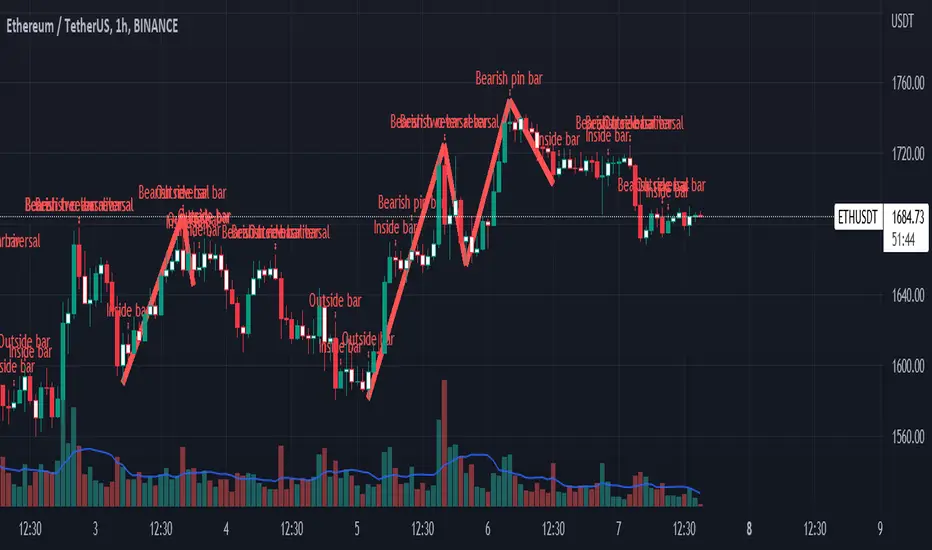
Symmetrical Geometric MandalaSymmetrical Geometric Mandala
Overview
The Symmetrical Geometric Mandala is an advanced geometric trading tool that applies phi (φ) harmonic relationships to price-time analysis. This indicator automatically detects swing ranges and constructs a scale-invariant geometric framework based on the square root of phi (√φ), revealing natural support/resistance zones and harmonic price-time balance points.
Core Concept
Traditional technical analysis often treats price and time as separate dimensions. This indicator harmonizes them using the mathematical constant √φ (approximately 1.272), creating a geometric "squaring" of price and time that remains proportionally consistent across different chart scales.
The Mathematics
When you select a price range (from swing low to swing high or vice versa), the indicator calculates:
PBR (Price-to-Bar Ratio) = Range / Number of Bars
Harmonic PBR = PBR × √φ (1.272019649514069)
Phi Extension = Range × φ (1.618033988749895)
The Harmonic PBR is the critical value - this is the chart scaling factor that creates perfect geometric harmony between price and time for your selected range.
Visual Components
1. Horizontal Boundary Lines
Two horizontal lines extend from the selected range at a distance of Range × φ (golden ratio extension):
Upper line: Extended above the swing high (for uplegs) or swing low (for downlegs)
Lower line: Extended below the swing low (for uplegs) or swing high (for downlegs)
These lines mark the natural harmonic boundaries of the price movement.
2. Rectangle Diagonal Lines
Two diagonal lines that create a "rectangle" effect, connecting:
Overlap points on horizontal boundaries to swing extremes
These lines go in the opposite direction of the price leg (creating the symmetrical mandala pattern)
When extended, they reveal future geometric support/resistance zones
3. Phi Harmonic Circles (Optional)
Two precisely calculated circles (drawn as smooth polylines):
Circle A: Centered at the first swing extreme (Nodal A)
Circle B: Centered at the second swing extreme (Nodal B)
Radius = Range × φ, causing them to perfectly touch the horizontal boundary lines
These circles visualize the geometric harmony and create a mandala-like pattern that reveals natural price zones.
How to Use
Step 1: Select Your Range
Set the Start Date at your swing low or swing high
Set the End Date at the opposite extreme
The indicator automatically detects whether it's an upleg or downleg
Step 2: Read the Harmonic PBR
Check the highlighted yellow row in the table: "PBR × √φ"
This is your chart scaling value
Step 3: Apply Chart Scaling (Optional)
For perfect geometric visualization:
Right-click on your chart's price axis
Select "Scale price chart only"
Enter the PBR × √φ value
The geometry will now display in perfect harmonic proportion
Step 4: Interpret the Geometry
Horizontal lines: Key support/resistance zones at phi extensions
Diagonal lines: Dynamic trend channels and future price-time balance points
Circle intersections: Natural harmonic turning points
Central diamond area: Core price-time equilibrium zone
Key Features
✅ Automatic swing detection - identifies upleg/downleg automatically
✅ Scale-invariant geometry - maintains proportions across timeframes
✅ Phi harmonic calculations - based on golden ratio mathematics
✅ Professional color scheme - clean, non-intrusive visuals
✅ Customizable display - toggle circles, lines, and table independently
✅ Smooth circle rendering - adjustable segments (16-360) for optimal smoothness
Settings
Show Horizontal Boundary Lines: Display phi extension levels
Show Rectangle Diagonal Lines: Display the geometric framework
Show Phi Harmonic Circles: Display circular geometry (optional)
Circle Smoothness: Adjust polyline segments (default: 96)
Colors: Fully customizable color scheme for all elements
Theory Background
This indicator draws inspiration from:
W.D. Gann's price-time squaring techniques
Bradley Cowan's geometric market analysis
Phi/golden ratio harmonic theory
Mathematical constants in market structure
Unlike traditional Fibonacci retracements, this tool uses √φ instead of φ as the primary scaling constant, creating a unique geometric relationship that "squares" price movement with time passage.
Best Practices
Use on significant swings - Works best on major swing highs/lows
Multiple timeframe analysis - Apply to different timeframes for confluence
Combine with other tools - Use alongside support/resistance and trend analysis
Respect the geometry - Pay attention when price interacts with geometric elements
Chart scaling optional - The geometry works at any scale, but scaling enhances visualization
Notes
The indicator draws geometry from left to right (from Nodal A to Nodal B)
All lines extend infinitely for future projections
The table shows real-time calculations for the selected range
Date range selection uses confirm dialogs to prevent accidental changes

Aetherium Institutional Market Resonance EngineAetherium Institutional Market Resonance Engine (AIMRE)
A Three-Pillar Framework for Decoding Institutional Activity
🎓 THEORETICAL FOUNDATION
The Aetherium Institutional Market Resonance Engine (AIMRE) is a multi-faceted analysis system designed to move beyond conventional indicators and decode the market's underlying structure as dictated by institutional capital flow. Its philosophy is built on a singular premise: significant market moves are preceded by a convergence of context , location , and timing . Aetherium quantifies these three dimensions through a revolutionary three-pillar architecture.
This system is not a simple combination of indicators; it is an integrated engine where each pillar's analysis feeds into a central logic core. A signal is only generated when all three pillars achieve a state of resonance, indicating a high-probability alignment between market organization, key liquidity levels, and cyclical momentum.
⚡ THE THREE-PILLAR ARCHITECTURE
1. 🌌 PILLAR I: THE COHERENCE ENGINE (THE 'CONTEXT')
Purpose: To measure the degree of organization within the market. This pillar answers the question: " Is the market acting with a unified purpose, or is it chaotic and random? "
Conceptual Framework: Institutional campaigns (accumulation or distribution) create a non-random, organized market environment. Retail-driven or directionless markets are characterized by "noise" and chaos. The Coherence Engine acts as a filter to ensure we only engage when institutional players are actively steering the market.
Formulaic Concept:
Coherence = f(Dominance, Synchronization)
Dominance Factor: Calculates the absolute difference between smoothed buying pressure (volume-weighted bullish candles) and smoothed selling pressure (volume-weighted bearish candles), normalized by total pressure. A high value signifies a clear winner between buyers and sellers.
Synchronization Factor: Measures the correlation between the streams of buying and selling pressure over the analysis window. A high positive correlation indicates synchronized, directional activity, while a negative correlation suggests choppy, conflicting action.
The final Coherence score (0-100) represents the percentage of market organization. A high score is a prerequisite for any signal, filtering out unpredictable market conditions.
2. 💎 PILLAR II: HARMONIC LIQUIDITY MATRIX (THE 'LOCATION')
Purpose: To identify and map high-impact institutional footprints. This pillar answers the question: " Where have institutions previously committed significant capital? "
Conceptual Framework: Large institutional orders leave indelible marks on the market in the form of anomalous volume spikes at specific price levels. These are not random occurrences but are areas of intense historical interest. The Harmonic Liquidity Matrix finds these footprints and consolidates them into actionable support and resistance zones called "Harmonic Nodes."
Algorithmic Process:
Footprint Identification: The engine scans the historical lookback period for candles where volume > average_volume * Institutional_Volume_Filter. This identifies statistically significant volume events.
Node Creation: A raw node is created at the mean price of the identified candle.
Dynamic Clustering: The engine uses an ATR-based proximity algorithm. If a new footprint is identified within Node_Clustering_Distance (ATR) of an existing Harmonic Node, it is merged. The node's price is volume-weighted, and its magnitude is increased. This prevents chart clutter and consolidates nearby institutional orders into a single, more significant level.
Node Decay: Nodes that are older than the Institutional_Liquidity_Scanback period are automatically removed from the chart, ensuring the analysis remains relevant to recent market dynamics.
3. 🌊 PILLAR III: CYCLICAL RESONANCE MATRIX (THE 'TIMING')
Purpose: To identify the market's dominant rhythm and its current phase. This pillar answers the question: " Is the market's immediate energy flowing up or down? "
Conceptual Framework: Markets move in waves and cycles of varying lengths. Trading in harmony with the current cyclical phase dramatically increases the probability of success. Aetherium employs a simplified wavelet analysis concept to decompose price action into short, medium, and long-term cycles.
Algorithmic Process:
Cycle Decomposition: The engine calculates three oscillators based on the difference between pairs of Exponential Moving Averages (e.g., EMA8-EMA13 for short cycle, EMA21-EMA34 for medium cycle).
Energy Measurement: The 'energy' of each cycle is determined by its recent volatility (standard deviation). The cycle with the highest energy is designated as the "Dominant Cycle."
Phase Analysis: The engine determines if the dominant cycles are in a bullish phase (rising from a trough) or a bearish phase (falling from a peak).
Cycle Sync: The highest conviction timing signals occur when multiple cycles (e.g., short and medium) are synchronized in the same direction, indicating broad-based momentum.
🔧 COMPREHENSIVE INPUT SYSTEM
Pillar I: Market Coherence Engine
Coherence Analysis Window (10-50, Default: 21): The lookback period for the Coherence Engine.
Lower Values (10-15): Highly responsive to rapid shifts in market control. Ideal for scalping but can be sensitive to noise.
Balanced (20-30): Excellent for day trading, capturing the ebb and flow of institutional sessions.
Higher Values (35-50): Smoother, more stable reading. Best for swing trading and identifying long-term institutional campaigns.
Coherence Activation Level (50-90%, Default: 70%): The minimum market organization required to enable signal generation.
Strict (80-90%): Only allows signals in extremely clear, powerful trends. Fewer, but potentially higher quality signals.
Standard (65-75%): A robust filter that effectively removes choppy conditions while capturing most valid institutional moves.
Lenient (50-60%): Allows signals in less-organized markets. Can be useful in ranging markets but may increase false signals.
Pillar II: Harmonic Liquidity Matrix
Institutional Liquidity Scanback (100-400, Default: 200): How far back the engine looks for institutional footprints.
Short (100-150): Focuses on recent institutional activity, providing highly relevant, immediate levels.
Long (300-400): Identifies major, long-term structural levels. These nodes are often extremely powerful but may be less frequent.
Institutional Volume Filter (1.3-3.0, Default: 1.8): The multiplier for detecting a volume spike.
High (2.5-3.0): Only registers climactic, undeniable institutional volume. Fewer, but more significant nodes.
Low (1.3-1.7): More sensitive, identifying smaller but still relevant institutional interest.
Node Clustering Distance (0.2-0.8 ATR, Default: 0.4): The ATR-based distance for merging nearby nodes.
High (0.6-0.8): Creates wider, more consolidated zones of liquidity.
Low (0.2-0.3): Creates more numerous, precise, and distinct levels.
Pillar III: Cyclical Resonance Matrix
Cycle Resonance Analysis (30-100, Default: 50): The lookback for determining cycle energy and dominance.
Short (30-40): Tunes the engine to faster, shorter-term market rhythms. Best for scalping.
Long (70-100): Aligns the timing component with the larger primary trend. Best for swing trading.
Institutional Signal Architecture
Signal Quality Mode (Professional, Elite, Supreme): Controls the strictness of the three-pillar confluence.
Professional: Loosest setting. May generate signals if two of the three pillars are in strong alignment. Increases signal frequency.
Elite: Balanced setting. Requires a clear, unambiguous resonance of all three pillars. The recommended default.
Supreme: Most stringent. Requires perfect alignment of all three pillars, with each pillar exhibiting exceptionally strong readings (e.g., coherence > 85%). The highest conviction signals.
Signal Spacing Control (5-25, Default: 10): The minimum bars between signals to prevent clutter and redundant alerts.
🎨 ADVANCED VISUAL SYSTEM
The visual architecture of Aetherium is designed not merely for aesthetics, but to provide an intuitive, at-a-glance understanding of the complex data being processed.
Harmonic Liquidity Nodes: The core visual element. Displayed as multi-layered, semi-transparent horizontal boxes.
Magnitude Visualization: The height and opacity of a node's "glow" are proportional to its volume magnitude. More significant nodes appear brighter and larger, instantly drawing the eye to key levels.
Color Coding: Standard nodes are blue/purple, while exceptionally high-magnitude nodes are highlighted in an accent color to denote critical importance.
🌌 Quantum Resonance Field: A dynamic background gradient that visualizes the overall market environment.
Color: Shifts from cool blues/purples (low coherence) to energetic greens/cyans (high coherence and organization), providing instant context.
Intensity: The brightness and opacity of the field are influenced by total market energy (a composite of coherence, momentum, and volume), making powerful market states visually apparent.
💎 Crystalline Lattice Matrix: A geometric web of lines projected from a central moving average.
Mathematical Basis: Levels are projected using multiples of the Golden Ratio (Phi ≈ 1.618) and the ATR. This visualizes the natural harmonic and fractal structure of the market. It is not arbitrary but is based on mathematical principles of market geometry.
🧠 Synaptic Flow Network: A dynamic particle system visualizing the engine's "thought process."
Node Density & Activation: The number of particles and their brightness/color are tied directly to the Market Coherence score. In high-coherence states, the network becomes a dense, bright, and organized web. In chaotic states, it becomes sparse and dim.
⚡ Institutional Energy Waves: Flowing sine waves that visualize market volatility and rhythm.
Amplitude & Speed: The height and speed of the waves are directly influenced by the ATR and volume, providing a feel for market energy.
📊 INSTITUTIONAL CONTROL MATRIX (DASHBOARD)
The dashboard is the central command console, providing a real-time, quantitative summary of each pillar's status.
Header: Displays the script title and version.
Coherence Engine Section:
State: Displays a qualitative assessment of market organization: ◉ PHASE LOCK (High Coherence), ◎ ORGANIZING (Moderate Coherence), or ○ CHAOTIC (Low Coherence). Color-coded for immediate recognition.
Power: Shows the precise Coherence percentage and a directional arrow (↗ or ↘) indicating if organization is increasing or decreasing.
Liquidity Matrix Section:
Nodes: Displays the total number of active Harmonic Liquidity Nodes currently being tracked.
Target: Shows the price level of the nearest significant Harmonic Node to the current price, representing the most immediate institutional level of interest.
Cycle Matrix Section:
Cycle: Identifies the currently dominant market cycle (e.g., "MID ") based on cycle energy.
Sync: Indicates the alignment of the cyclical forces: ▲ BULLISH , ▼ BEARISH , or ◆ DIVERGENT . This is the core timing confirmation.
Signal Status Section:
A unified status bar that provides the final verdict of the engine. It will display "QUANTUM SCAN" during neutral periods, or announce the tier and direction of an active signal (e.g., "◉ TIER 1 BUY ◉" ), highlighted with the appropriate color.
🎯 SIGNAL GENERATION LOGIC
Aetherium's signal logic is built on the principle of strict, non-negotiable confluence.
Condition 1: Context (Coherence Filter): The Market Coherence must be above the Coherence Activation Level. No signals can be generated in a chaotic market.
Condition 2: Location (Liquidity Node Interaction): Price must be actively interacting with a significant Harmonic Liquidity Node.
For a Buy Signal: Price must be rejecting the Node from below (testing it as support).
For a Sell Signal: Price must be rejecting the Node from above (testing it as resistance).
Condition 3: Timing (Cycle Alignment): The Cyclical Resonance Matrix must confirm that the dominant cycles are synchronized with the intended trade direction.
Signal Tiering: The Signal Quality Mode input determines how strictly these three conditions must be met. 'Supreme' mode, for example, might require not only that the conditions are met, but that the Market Coherence is exceptionally high and the interaction with the Node is accompanied by a significant volume spike.
Signal Spacing: A final filter ensures that signals are spaced by a minimum number of bars, preventing over-alerting in a single move.
🚀 ADVANCED TRADING STRATEGIES
The Primary Confluence Strategy: The intended use of the system. Wait for a Tier 1 (Elite/Supreme) or Tier 2 (Professional/Elite) signal to appear on the chart. This represents the alignment of all three pillars. Enter after the signal bar closes, with a stop-loss placed logically on the other side of the Harmonic Node that triggered the signal.
The Coherence Context Strategy: Use the Coherence Engine as a standalone market filter. When Coherence is high (>70%), favor trend-following strategies. When Coherence is low (<50%), avoid new directional trades or favor range-bound strategies. A sharp drop in Coherence during a trend can be an early warning of a trend's exhaustion.
Node-to-Node Trading: In a high-coherence environment, use the Harmonic Liquidity Nodes as both entry points and profit targets. For example, after a BUY signal is generated at one Node, the next Node above it becomes a logical first profit target.
⚖️ RESPONSIBLE USAGE AND LIMITATIONS
Decision Support, Not a Crystal Ball: Aetherium is an advanced decision-support tool. It is designed to identify high-probability conditions based on a model of institutional behavior. It does not predict the future.
Risk Management is Paramount: No indicator can replace a sound risk management plan. Always use appropriate position sizing and stop-losses. The signals provided are probabilistic, not certainties.
Past Performance Disclaimer: The market models used in this script are based on historical data. While robust, there is no guarantee that these patterns will persist in the future. Market conditions can and do change.
Not a "Set and Forget" System: The indicator performs best when its user understands the concepts behind the three pillars. Use the dashboard and visual cues to build a comprehensive view of the market before acting on a signal.
Backtesting is Essential: Before applying this tool to live trading, it is crucial to backtest and forward-test it on your preferred instruments and timeframes to understand its unique behavior and characteristics.
🔮 CONCLUSION
The Aetherium Institutional Market Resonance Engine represents a paradigm shift from single-variable analysis to a holistic, multi-pillar framework. By quantifying the abstract concepts of market context, location, and timing into a unified, logical system, it provides traders with an unprecedented lens into the mechanics of institutional market operations.
It is not merely an indicator, but a complete analytical engine designed to foster a deeper understanding of market dynamics. By focusing on the core principles of institutional order flow, Aetherium empowers traders to filter out market noise, identify key structural levels, and time their entries in harmony with the market's underlying rhythm.
"In all chaos there is a cosmos, in all disorder a secret order." - Carl Jung
— Dskyz, Trade with insight. Trade with confluence. Trade with Aetherium.

IU Market Rhythm WaveDESCRIPTION:
The IU Market Rhythm Wave is a multi-dimensional indicator designed to reveal the underlying rhythm and energy of the market. By analyzing price momentum, harmonic oscillations, volume behavior, and market breadth, it helps traders identify high-quality long and short wave signals. It also visualizes rhythm bands, wave strength zones, and harmonic levels to provide comprehensive context for decision-making.
This tool is best used on trending instruments where rhythm cycles and volume patterns create clear wave-based opportunities.
USER INPUTS:
Rhythm Cycle Length
Controls the main lookback period used to calculate price waves, harmonic oscillation, volume rhythm, and breath. A longer cycle smooths signals, while a shorter cycle makes them more responsive. Recommended range: 8 to 35.
Wave Signal Strength
Multiplies the standard deviation of rhythm to define dynamic breakout thresholds. A higher value results in fewer but stronger signals, filtering out minor fluctuations.
Harmonic Filter
Applies a sensitivity filter to the harmonic mean and standard deviation. It helps eliminate weak or noisy signals and ensures rhythm-based signals align with harmonic structure.
Show Wave Energy Zones
Toggles background color shading based on current rhythm conditions. Greenish zones indicate strong upward rhythm, red for strong downward rhythm, yellow for positive bias, and gray for weak or neutral zones.
Show Rhythm Bands
Enables the display of upper and lower rhythm bands derived from ATR and rhythm volatility. These bands act as dynamic price envelopes and potential support/resistance zones.
Wave Zone Opacity
Adjusts the transparency of background energy zones, allowing users to control how prominent these zones appear on the chart. Range: 60 to 90 for optimal visibility.
INDICATOR LOGIC:
The indicator combines multiple rhythmic components into a composite rhythm score:
1. Price Wave – Based on momentum (rate of price change) smoothed by a moving average.
2. Harmonic Oscillation – Measures how far price has deviated from a central harmonic average (HLC3).
3. Volume Rhythm – Uses volume’s deviation from its mean, standardized by its volatility.
4. Market Breath – Captures range expansion and closing strength relative to range.
These elements form the Raw Rhythm, which is further smoothed to produce the Market Rhythm. When the rhythm exceeds statistically calculated thresholds and other conditions like volume confirmation and harmonic proximity are met, wave signals are triggered.
Harmonic Fibonacci levels (0.236, 0.382, 0.618, 0.764) are also calculated every rhythm cycle to identify nearby structural price zones. Signals occurring near these levels are considered more reliable.
The Rhythm Bands use ATR and rhythm strength to define dynamic boundaries above and below price. Visual zones and arrows mark rhythm shifts and highlight the underlying energy of the market.
WHY IT IS UNIQUE:
This indicator goes beyond traditional oscillators or volume indicators by blending multiple market dimensions into one rhythmic framework. It adapts to volatility, applies harmonic structure awareness, and filters signals based on real-time market conditions. It offers:
* A unique rhythm-based view of price, volume, and volatility
* Dynamic, adaptive signal generation and zone coloring
* Visual analytics and contextual data in a summary table
* Signal filtering using harmonic alignment and market breath
Its real-time responsiveness and multi-layered logic make it suitable for intraday, swing, and positional traders.
HOW USER CAN BENEFIT FROM IT:
* Spot high-conviction long or short entries when rhythm, volume, and structure align
* Avoid low-quality trades during weak or noisy rhythm periods
* Use visual wave zones to gauge trend strength and rhythm direction
* Monitor harmonic proximity to enter or exit near key structural levels
* Apply rhythm bands for dynamic stop-loss and target setting
* Use rhythm direction arrows and analytics table to gain deeper market insight
DISCLAIMER:
This indicator is created for educational and informational purposes only. It does not constitute financial advice or a recommendation to buy or sell any asset. All trading involves risk, and users should conduct their own analysis or consult with a qualified financial advisor before making any trading decisions. The creator is not responsible for any losses incurred through the use of this tool. Use at your own discretion.
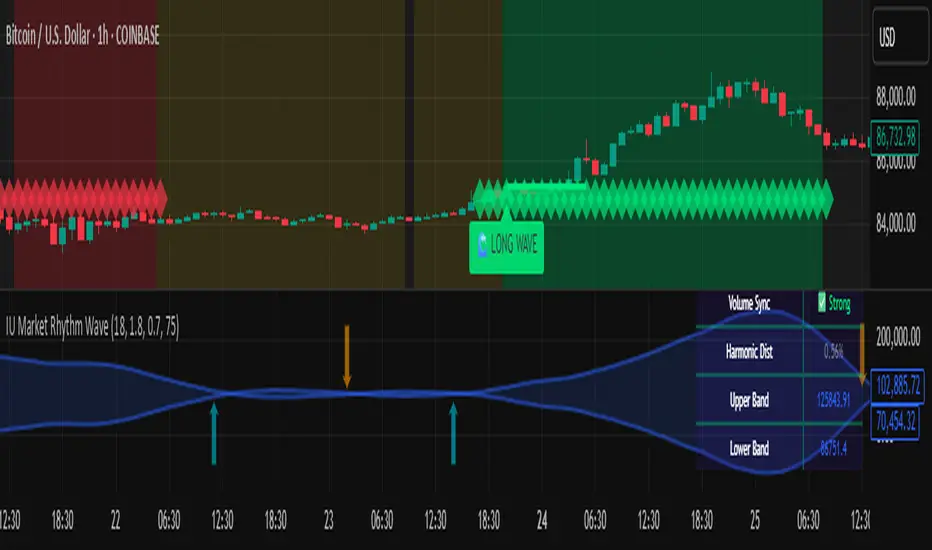
Langlands-Operadic Möbius Vortex (LOMV)Langlands-Operadic Möbius Vortex (LOMV)
Where Pure Mathematics Meets Market Reality
A Revolutionary Synthesis of Number Theory, Category Theory, and Market Dynamics
🎓 THEORETICAL FOUNDATION
The Langlands-Operadic Möbius Vortex represents a groundbreaking fusion of three profound mathematical frameworks that have never before been combined for market analysis:
The Langlands Program: Harmonic Analysis in Markets
Developed by Robert Langlands (Fields Medal recipient), the Langlands Program creates bridges between number theory, algebraic geometry, and harmonic analysis. In our indicator:
L-Function Implementation:
- Utilizes the Möbius function μ(n) for weighted price analysis
- Applies Riemann zeta function convergence principles
- Calculates quantum harmonic resonance between -2 and +2
- Measures deep mathematical patterns invisible to traditional analysis
The L-Function core calculation employs:
L_sum = Σ(return_val × μ(n) × n^(-s))
Where s is the critical strip parameter (0.5-2.5), controlling mathematical precision and signal smoothness.
Operadic Composition Theory: Multi-Strategy Democracy
Category theory and operads provide the mathematical framework for composing multiple trading strategies into a unified signal. This isn't simple averaging - it's mathematical composition using:
Strategy Composition Arity (2-5 strategies):
- Momentum analysis via RSI transformation
- Mean reversion through Bollinger Band mathematics
- Order Flow Polarity Index (revolutionary T3-smoothed volume analysis)
- Trend detection using Directional Movement
- Higher timeframe momentum confirmation
Agreement Threshold System: Democratic voting where strategies must reach consensus before signal generation. This prevents false signals during market uncertainty.
Möbius Function: Number Theory in Action
The Möbius function μ(n) forms the mathematical backbone:
- μ(n) = 1 if n is a square-free positive integer with even number of prime factors
- μ(n) = -1 if n is a square-free positive integer with odd number of prime factors
- μ(n) = 0 if n has a squared prime factor
This creates oscillating weights that reveal hidden market periodicities and harmonic structures.
🔧 COMPREHENSIVE INPUT SYSTEM
Langlands Program Parameters
Modular Level N (5-50, default 30):
Primary lookback for quantum harmonic analysis. Optimized by timeframe:
- Scalping (1-5min): 15-25
- Day Trading (15min-1H): 25-35
- Swing Trading (4H-1D): 35-50
- Asset-specific: Crypto 15-25, Stocks 30-40, Forex 35-45
L-Function Critical Strip (0.5-2.5, default 1.5):
Controls Riemann zeta convergence precision:
- Higher values: More stable, smoother signals
- Lower values: More reactive, catches quick moves
- High frequency: 0.8-1.2, Medium: 1.3-1.7, Low: 1.8-2.3
Frobenius Trace Period (5-50, default 21):
Galois representation lookback for price-volume correlation:
- Measures harmonic relationships in market flows
- Scalping: 8-15, Day Trading: 18-25, Swing: 25-40
HTF Multi-Scale Analysis:
Higher timeframe context prevents trading against major trends:
- Provides market bias and filters signals
- Improves win rates by 15-25% through trend alignment
Operadic Composition Parameters
Strategy Composition Arity (2-5, default 4):
Number of algorithms composed for final signal:
- Conservative: 4-5 strategies (higher confidence)
- Moderate: 3-4 strategies (balanced approach)
- Aggressive: 2-3 strategies (more frequent signals)
Category Agreement Threshold (2-5, default 3):
Democratic voting minimum for signal generation:
- Higher agreement: Fewer but higher quality signals
- Lower agreement: More signals, potential false positives
Swiss-Cheese Mixing (0.1-0.5, default 0.382):
Golden ratio φ⁻¹ based blending of trend factors:
- 0.382 is φ⁻¹, optimal for natural market fractals
- Higher values: Stronger trend following
- Lower values: More contrarian signals
OFPI Configuration:
- OFPI Length (5-30, default 14): Order Flow calculation period
- T3 Smoothing (3-10, default 5): Advanced exponential smoothing
- T3 Volume Factor (0.5-1.0, default 0.7): Smoothing aggressiveness control
Unified Scoring System
Component Weights (sum ≈ 1.0):
- L-Function Weight (0.1-0.5, default 0.3): Mathematical harmony emphasis
- Galois Rank Weight (0.1-0.5, default 0.2): Market structure complexity
- Operadic Weight (0.1-0.5, default 0.3): Multi-strategy consensus
- Correspondence Weight (0.1-0.5, default 0.2): Theory-practice alignment
Signal Threshold (0.5-10.0, default 5.0):
Quality filter producing:
- 8.0+: EXCEPTIONAL signals only
- 6.0-7.9: STRONG signals
- 4.0-5.9: MODERATE signals
- 2.0-3.9: WEAK signals
🎨 ADVANCED VISUAL SYSTEM
Multi-Dimensional Quantum Aura Bands
Five-layer resonance field showing market energy:
- Colors: Theme-matched gradients (Quantum purple, Holographic cyan, etc.)
- Expansion: Dynamic based on score intensity and volatility
- Function: Multi-timeframe support/resistance zones
Morphism Flow Portals
Category theory visualization showing market topology:
- Green/Cyan Portals: Bullish mathematical flow
- Red/Orange Portals: Bearish mathematical flow
- Size/Intensity: Proportional to signal strength
- Recursion Depth (1-8): Nested patterns for flow evolution
Fractal Grid System
Dynamic support/resistance with projected L-Scores:
- Multiple Timeframes: 10, 20, 30, 40, 50-period highs/lows
- Smart Spacing: Prevents level overlap using ATR-based minimum distance
- Projections: Estimated signal scores when price reaches levels
- Usage: Precise entry/exit timing with mathematical confirmation
Wick Pressure Analysis
Rejection level prediction using candle mathematics:
- Upper Wicks: Selling pressure zones (purple/red lines)
- Lower Wicks: Buying pressure zones (purple/green lines)
- Glow Intensity (1-8): Visual emphasis and line reach
- Application: Confluence with fractal grid creates high-probability zones
Regime Intensity Heatmap
Background coloring showing market energy:
- Black/Dark: Low activity, range-bound markets
- Purple Glow: Building momentum and trend development
- Bright Purple: High activity, strong directional moves
- Calculation: Combines trend, momentum, volatility, and score intensity
Six Professional Themes
- Quantum: Purple/violet for general trading and mathematical focus
- Holographic: Cyan/magenta optimized for cryptocurrency markets
- Crystalline: Blue/turquoise for conservative, stability-focused trading
- Plasma: Gold/magenta for high-energy volatility trading
- Cosmic Neon: Bright neon colors for maximum visibility and aggressive trading
📊 INSTITUTIONAL-GRADE DASHBOARD
Unified AI Score Section
- Total Score (-10 to +10): Primary decision metric
- >5: Strong bullish signals
- <-5: Strong bearish signals
- Quality ratings: EXCEPTIONAL > STRONG > MODERATE > WEAK
- Component Analysis: Individual L-Function, Galois, Operadic, and Correspondence contributions
Order Flow Analysis
Revolutionary OFPI integration:
- OFPI Value (-100% to +100%): Real buying vs selling pressure
- Visual Gauge: Horizontal bar chart showing flow intensity
- Momentum Status: SHIFTING, ACCELERATING, STRONG, MODERATE, or WEAK
- Trading Application: Flow shifts often precede major moves
Signal Performance Tracking
- Win Rate Monitoring: Real-time success percentage with emoji indicators
- Signal Count: Total signals generated for frequency analysis
- Current Position: LONG, SHORT, or NONE with P&L tracking
- Volatility Regime: HIGH, MEDIUM, or LOW classification
Market Structure Analysis
- Möbius Field Strength: Mathematical field oscillation intensity
- CHAOTIC: High complexity, use wider stops
- STRONG: Active field, normal position sizing
- MODERATE: Balanced conditions
- WEAK: Low activity, consider smaller positions
- HTF Trend: Higher timeframe bias (BULL/BEAR/NEUTRAL)
- Strategy Agreement: Multi-algorithm consensus level
Position Management
When in trades, displays:
- Entry Price: Original signal price
- Current P&L: Real-time percentage with risk level assessment
- Duration: Bars in trade for timing analysis
- Risk Level: HIGH/MEDIUM/LOW based on current exposure
🚀 SIGNAL GENERATION LOGIC
Balanced Long/Short Architecture
The indicator generates signals through multiple convergent pathways:
Long Entry Conditions:
- Score threshold breach with algorithmic agreement
- Strong bullish order flow (OFPI > 0.15) with positive composite signal
- Bullish pattern recognition with mathematical confirmation
- HTF trend alignment with momentum shifting
- Extreme bullish OFPI (>0.3) with any positive score
Short Entry Conditions:
- Score threshold breach with bearish agreement
- Strong bearish order flow (OFPI < -0.15) with negative composite signal
- Bearish pattern recognition with mathematical confirmation
- HTF trend alignment with momentum shifting
- Extreme bearish OFPI (<-0.3) with any negative score
Exit Logic:
- Score deterioration below continuation threshold
- Signal quality degradation
- Opposing order flow acceleration
- 10-bar minimum between signals prevents overtrading
⚙️ OPTIMIZATION GUIDELINES
Asset-Specific Settings
Cryptocurrency Trading:
- Modular Level: 15-25 (capture volatility)
- L-Function Precision: 0.8-1.3 (reactive to price swings)
- OFPI Length: 10-20 (fast correlation shifts)
- Cascade Levels: 5-7, Theme: Holographic
Stock Index Trading:
- Modular Level: 25-35 (balanced trending)
- L-Function Precision: 1.5-1.8 (stable patterns)
- OFPI Length: 14-20 (standard correlation)
- Cascade Levels: 4-5, Theme: Quantum
Forex Trading:
- Modular Level: 35-45 (smooth trends)
- L-Function Precision: 1.6-2.1 (high smoothing)
- OFPI Length: 18-25 (disable volume amplification)
- Cascade Levels: 3-4, Theme: Crystalline
Timeframe Optimization
Scalping (1-5 minute charts):
- Reduce all lookback parameters by 30-40%
- Increase L-Function precision for noise reduction
- Enable all visual elements for maximum information
- Use Small dashboard to save screen space
Day Trading (15 minute - 1 hour):
- Use default parameters as starting point
- Adjust based on market volatility
- Normal dashboard provides optimal information density
- Focus on OFPI momentum shifts for entries
Swing Trading (4 hour - Daily):
- Increase lookback parameters by 30-50%
- Higher L-Function precision for stability
- Large dashboard for comprehensive analysis
- Emphasize HTF trend alignment
🏆 ADVANCED TRADING STRATEGIES
The Mathematical Confluence Method
1. Wait for Fractal Grid level approach
2. Confirm with projected L-Score > threshold
3. Verify OFPI alignment with direction
4. Enter on portal signal with quality ≥ STRONG
5. Exit on score deterioration or opposing flow
The Regime Trading System
1. Monitor Aether Flow background intensity
2. Trade aggressively during bright purple periods
3. Reduce position size during dark periods
4. Use Möbius Field strength for stop placement
5. Align with HTF trend for maximum probability
The OFPI Momentum Strategy
1. Watch for momentum shifting detection
2. Confirm with accelerating flow in direction
3. Enter on immediate portal signal
4. Scale out at Fibonacci levels
5. Exit on flow deceleration or reversal
⚠️ RISK MANAGEMENT INTEGRATION
Mathematical Position Sizing
- Use Galois Rank for volatility-adjusted sizing
- Möbius Field strength determines stop width
- Fractal Dimension guides maximum exposure
- OFPI momentum affects entry timing
Signal Quality Filtering
- Trade only STRONG or EXCEPTIONAL quality signals
- Increase position size with higher agreement levels
- Reduce risk during CHAOTIC Möbius field periods
- Respect HTF trend alignment for directional bias
🔬 DEVELOPMENT JOURNEY
Creating the LOMV was an extraordinary mathematical undertaking that pushed the boundaries of what's possible in technical analysis. This indicator almost didn't happen. The theoretical complexity nearly proved insurmountable.
The Mathematical Challenge
Implementing the Langlands Program required deep research into:
- Number theory and the Möbius function
- Riemann zeta function convergence properties
- L-function analytical continuation
- Galois representations in finite fields
The mathematical literature spans decades of pure mathematics research, requiring translation from abstract theory to practical market application.
The Computational Complexity
Operadic composition theory demanded:
- Category theory implementation in Pine Script
- Multi-dimensional array management for strategy composition
- Real-time democratic voting algorithms
- Performance optimization for complex calculations
The Integration Breakthrough
Bringing together three disparate mathematical frameworks required:
- Novel approaches to signal weighting and combination
- Revolutionary Order Flow Polarity Index development
- Advanced T3 smoothing implementation
- Balanced signal generation preventing directional bias
Months of intensive research culminated in breakthrough moments when the mathematics finally aligned with market reality. The result is an indicator that reveals market structure invisible to conventional analysis while maintaining practical trading utility.
🎯 PRACTICAL IMPLEMENTATION
Getting Started
1. Apply indicator with default settings
2. Select appropriate theme for your markets
3. Observe dashboard metrics during different market conditions
4. Practice signal identification without trading
5. Gradually adjust parameters based on observations
Signal Confirmation Process
- Never trade on score alone - verify quality rating
- Confirm OFPI alignment with intended direction
- Check fractal grid level proximity for timing
- Ensure Möbius field strength supports position size
- Validate against HTF trend for bias confirmation
Performance Monitoring
- Track win rate in dashboard for strategy assessment
- Monitor component contributions for optimization
- Adjust threshold based on desired signal frequency
- Document performance across different market regimes
🌟 UNIQUE INNOVATIONS
1. First Integration of Langlands Program mathematics with practical trading
2. Revolutionary OFPI with T3 smoothing and momentum detection
3. Operadic Composition using category theory for signal democracy
4. Dynamic Fractal Grid with projected L-Score calculations
5. Multi-Dimensional Visualization through morphism flow portals
6. Regime-Adaptive Background showing market energy intensity
7. Balanced Signal Generation preventing directional bias
8. Professional Dashboard with institutional-grade metrics
📚 EDUCATIONAL VALUE
The LOMV serves as both a practical trading tool and an educational gateway to advanced mathematics. Traders gain exposure to:
- Pure mathematics applications in markets
- Category theory and operadic composition
- Number theory through Möbius function implementation
- Harmonic analysis via L-function calculations
- Advanced signal processing through T3 smoothing
⚖️ RESPONSIBLE USAGE
This indicator represents advanced mathematical research applied to market analysis. While the underlying mathematics are rigorously implemented, markets remain inherently unpredictable.
Key Principles:
- Use as part of comprehensive trading strategy
- Implement proper risk management at all times
- Backtest thoroughly before live implementation
- Understand that past performance does not guarantee future results
- Never risk more than you can afford to lose
The mathematics reveal deep market structure, but successful trading requires discipline, patience, and sound risk management beyond any indicator.
🔮 CONCLUSION
The Langlands-Operadic Möbius Vortex represents a quantum leap forward in technical analysis, bringing PhD-level pure mathematics to practical trading while maintaining visual elegance and usability.
From the harmonic analysis of the Langlands Program to the democratic composition of operadic theory, from the number-theoretic precision of the Möbius function to the revolutionary Order Flow Polarity Index, every component works in mathematical harmony to reveal the hidden order within market chaos.
This is more than an indicator - it's a mathematical lens that transforms how you see and understand market structure.
Trade with mathematical precision. Trade with the LOMV.
*"Mathematics is the language with which God has written the universe." - Galileo Galilei*
*In markets, as in nature, profound mathematical beauty underlies apparent chaos. The LOMV reveals this hidden order.*
— Dskyz, Trade with insight. Trade with anticipation.

WaveFunction MACD (TechnoBlooms)WaveFunction MACD — The Next Generation of Market Momentum
WaveFunction MACD is an advanced hybrid momentum indicator that merges:
• The classical MACD crossover logic (based on moving averages)
• Wave physics (modeled through phase energy and cosine functions)
• Hilbert Transform theory from signal processing
• The concept of a wavefunction from quantum mechanics, where price action is seen as a probabilistic energy wave—not just a trend.
✨ Key Features of WaveFunction MACD
• Wave Energy Logic : Instead of using just price and MA differences, this indicator computes phase-corrected momentum using the cosine of the wave phase angle — revealing the true energy behind market moves.
• Phase-Based Trend Detection : It reads cycle phases using Hilbert Transform-like logic, allowing you to spot momentum before it becomes visible in price.
• Ultra-Smooth Flow : The main line and histogram are built to follow price flow smoothly — eliminating much of the noise found in traditional MACD indicators.
• Signal Amplification via Energy Histogram : The histogram doesn’t just show momentum changes — it shows the intensity of wave energy, allowing you to confirm the strength of the trend.
• Physics-Driven Structure : The algorithm is rooted in real-world wave mechanics, bringing a scientific edge to trading — ideal for traders who believe in natural models like cycles and harmonics.
• Trend Confirmation & Early Reversals : It can confirm strong trends and also catch subtle shifts that often precede big reversals — giving you both reliability and anticipation.
• Ready for Fusion : Designed to work seamlessly with liquidity zones, price action, order blocks, and structure trading — a perfect fit for modern trading systems.
🧪 The Science Behind It
This tool blends:
• Hilbert Transform: Measures the phase of a waveform (price cycle) to detect turning points
• Cosine Phase Energy: Calculates true wave energy using the cosine of the phase angle, revealing the strength behind price movements
• Quantum Modeling: Views price like a wavefunction, offering predictive insight based on phase dynamics

HarmonicMapLibLibrary "HarmonicMapLib"
Harmonic Pattern Library implementation utilising maps
method tostring(this)
convert Range value to string
Namespace types: Range
Parameters:
this (Range) : Range value
Returns: converted string representation
method tostring(this)
convert array of Range value to string
Namespace types: array
Parameters:
this (array) : array object
Returns: converted string representation
method tostring(this)
convert map of string to Range value to string
Namespace types: map
Parameters:
this (map) : map object
Returns: converted string representation
method tostring(this)
convert RatioMap to string
Namespace types: RatioMap
Parameters:
this (RatioMap) : RatioMap object
Returns: converted string representation
method tostring(this)
convert array of RatioMap to string
Namespace types: array
Parameters:
this (array) : array object
Returns: converted string representation
method tostring(this)
convert map of string to RatioMap to string
Namespace types: map
Parameters:
this (map) : map object
Returns: converted string representation
method tostring(this)
convert map of string to bool to string
Namespace types: map
Parameters:
this (map) : map object
Returns: converted string representation
method tostring(this)
convert PrzRange to string
Namespace types: PrzRange
Parameters:
this (PrzRange) : PrzRange object
Returns: converted string representation
method tostring(this)
convert array of PrzRange to string
Namespace types: array
Parameters:
this (array) : array object
Returns: converted string representation
getHarmonicMap()
Creates the RatioMap for harmonic patterns
Returns: map haronic ratio rules for all patterns
method evaluate(patternsMap, pattern, ratioRange, properties, ratioValue)
evaluates harmonic ratio range
Namespace types: map
Parameters:
patternsMap (map) : parameter containing valid pattern names
pattern (string) : Pattern type to be evaluated
ratioRange (Range) : ratio range to be checked
properties (ScanProperties) : Scan Properties
ratioValue (float)
Returns: void
method evaluate(przRange, pattern, ratioRange, priceRange, properties)
Evaluate PRZ ranges
Namespace types: map
Parameters:
przRange (map)
pattern (string) : Pattern name
ratioRange (Range) : Range of ratio for the pattern
priceRange (Range) : Price range based on ratio
properties (ScanProperties) : ScanProperties object
Returns: void
method scanRatio(currentPatterns, rules, properties, ratioName, ratioValue)
Scan for particular named ratio of harmonic pattern to filter valid patterns
Namespace types: map
Parameters:
currentPatterns (map) : Current valid patterns map
rules (map) : map Harmonic ratio rules
properties (ScanProperties) : ScanProperties object
ratioName (string) : Specific ratio name
ratioValue (float) : ratio value to be checked
Returns: updated currentPatterns object
method scanPatterns(patterns, x, a, b, c, d, properties)
Scan for patterns based on X, A, B, C, D values
Namespace types: map
Parameters:
patterns (map) : List of allowed patterns
x (float) : X coordinate
a (float) : A coordinate
b (float) : B coordinate
c (float) : C coordinate
d (float) : D coordinate
properties (ScanProperties) : ScanProperties object. If na, default values are initialised
Returns: updated valid patterns map
method scanProjections(patterns, x, a, b, c, properties)
Scan for projections based on X, A, B, C values
Namespace types: map
Parameters:
patterns (map) : List of allowed patterns
x (float) : X coordinate
a (float) : A coordinate
b (float) : B coordinate
c (float) : C coordinate
properties (ScanProperties) : ScanProperties object. If na, default values are initialised
Returns: updated valid projections map
method merge(this, other)
merge two ranges into one
Namespace types: Range
Parameters:
this (Range) : first range
other (Range) : second range
Returns: combined range
method union(this, other)
union of two ranges into one
Namespace types: Range
Parameters:
this (Range) : first range
other (Range) : second range
Returns: union range
method overlaps(this, other)
checks if two ranges intersect
Namespace types: Range
Parameters:
this (Range) : first range
other (Range) : second range
Returns: true if intersects, false otherwise
method consolidate(this)
Consolidate ranges into PRZ
Namespace types: map
Parameters:
this (map) : map of Ranges
Returns: consolidated PRZ
method consolidateMany(this)
Consolidate ranges into multiple PRZ ranges
Namespace types: map
Parameters:
this (map) : map of Ranges
Returns: consolidated array of PRZ ranges
method getRange(currentPatterns, x, a, b, c, properties)
Get D range based on X, A, B, C coordinates for the current patterns
Namespace types: map
Parameters:
currentPatterns (map) : List of valid patterns
x (float) : X coordinate
a (float) : A coordinate
b (float) : B coordinate
c (float) : C coordinate
properties (ScanProperties) : ScanProperties object. If na, default values are initialised
Returns: map of D ranges
method getPrzRange(currentPatterns, x, a, b, c, properties)
Get PRZ range based on X, A, B, C coordinates for the current patterns
Namespace types: map
Parameters:
currentPatterns (map) : List of valid patterns
x (float) : X coordinate
a (float) : A coordinate
b (float) : B coordinate
c (float) : C coordinate
properties (ScanProperties) : ScanProperties object. If na, default values are initialised
Returns: PRZRange for the pattern
method getProjectionRanges(currentPatterns, x, a, b, c, properties)
Get projection range based on X, A, B, C coordinates for the current patterns
Namespace types: map
Parameters:
currentPatterns (map) : List of valid patterns
x (float) : X coordinate
a (float) : A coordinate
b (float) : B coordinate
c (float) : C coordinate
properties (ScanProperties) : ScanProperties object. If na, default values are initialised
Returns: array of projection ranges
Range
Collection of range values
Fields:
values (array) : array of float values
RatioMap
ratio map for pattern
Fields:
ratioMap (map) : map of string to Range (array of float)
ScanProperties
Pattern Scanning properties
Fields:
strictMode (series bool) : strict scanning mode will check for overflows
logScale (series bool) : scan ratios in log scale
errorMin (series float) : min error threshold
errorMax (series float)
mintick (series float) : minimum tick value of price
PrzRange
Potential reversal zone range
Fields:
patterns (array) : array of pattern names for the given XABCD combination
prz (Range) : PRZ range
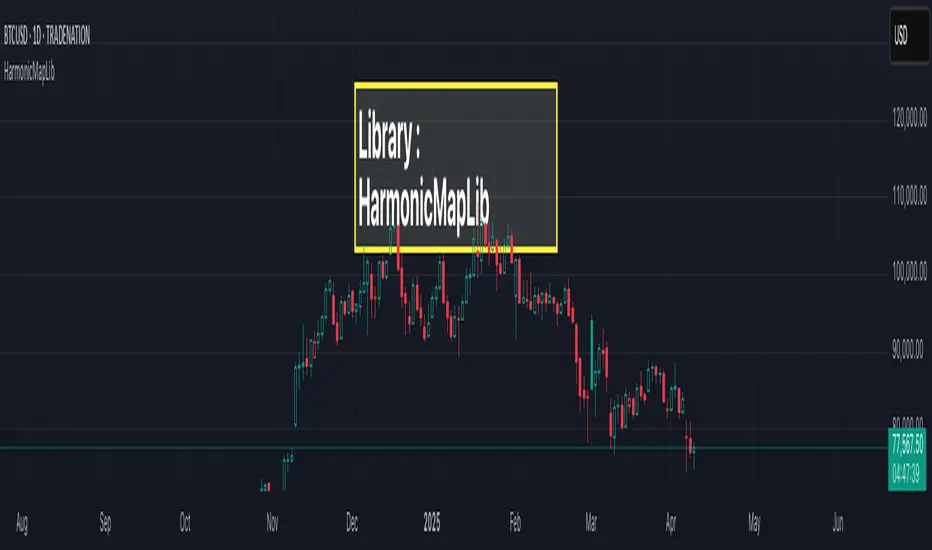
Adaptive Fourier Transform Supertrend [QuantAlgo]Discover a brand new way to analyze trend with Adaptive Fourier Transform Supertrend by QuantAlgo , an innovative technical indicator that combines the power of Fourier analysis with dynamic Supertrend methodology. In essence, it utilizes the frequency domain mathematics and the adaptive volatility control technique to transform complex wave patterns into clear and high probability signals—ideal for both sophisticated traders seeking mathematical precision and investors who appreciate robust trend confirmation!
🟢 Core Architecture
At its core, this indicator employs an adaptive Fourier Transform framework with dynamic volatility-controlled Supertrend bands. It utilizes multiple harmonic components that let you fine-tune how market frequencies influence trend detection. By combining wave analysis with adaptive volatility bands, the indicator creates a sophisticated yet clear framework for trend identification that dynamically adjusts to changing market conditions.
🟢 Technical Foundation
The indicator builds on three innovative components:
Fourier Wave Analysis: Decomposes price action into primary and harmonic components for precise trend detection
Adaptive Volatility Control: Dynamically adjusts Supertrend bands using combined ATR and standard deviation
Harmonic Integration: Merges multiple frequency components with decreasing weights for comprehensive trend analysis
🟢 Key Features & Signals
The Adaptive Fourier Transform Supertrend transforms complex wave calculations into clear visual signals with:
Dynamic trend bands that adapt to market volatility
Sophisticated cloud-fill visualization system
Strategic L/S markers at key trend reversals
Customizable bar coloring based on trend direction
Comprehensive alert system for trend shifts
🟢 Practical Usage Tips
Here's how you can get the most out of the Adaptive Fourier Transform Supertrend :
1/ Setup:
Add the indicator to your favorites, then apply it to your chart ⭐️
Start with close price as your base source
Use standard Fourier period (14) for balanced wave detection
Begin with default harmonic weight (0.5) for balanced sensitivity
Start with standard Supertrend multiplier (2.0) for reliable band width
2/ Signal Interpretation:
Monitor trend band crossovers for potential signals
Watch for convergence of price with Fourier trend
Use L/S markers for trade entry points
Monitor bar colors for trend confirmation
Configure alerts for significant trend reversals
🟢 Pro Tips
Fine-tune Fourier parameters for optimal sensitivity:
→ Lower Base Period (8-12) for more reactive analysis
→ Higher Base Period (15-30) to filter out noise
→ Adjust Harmonic Weight (0.3-0.7) to control shorter trend influence
Customize Supertrend settings:
→ Lower multiplier (1.5-2.0) for tighter bands
→ Higher multiplier (2.0-3.0) for wider bands
→ Adjust ATR length based on market volatility
Strategy Enhancement:
→ Compare signals across multiple timeframes
→ Combine with volume analysis
→ Use with support/resistance levels
→ Integrate with other momentum indicators

Obj_XABCD_HarmonicLibrary "Obj_XABCD_Harmonic"
Harmonic XABCD Pattern object and associated methods. Easily validate, draw, and get information about harmonic patterns. See example code at the end of the script for details.
init_params(pct_error, pct_asym, types, w_e, w_p, w_d)
Create a harmonic parameters object (used by xabcd_harmonic object for pattern validation and scoring).
Parameters:
pct_error : Allowed % error of leg retracement ratio versus the defined harmonic ratio
pct_asym : Allowed leg length/period asymmetry % (a leg is considered invalid if it is this % longer or shorter than the average length of the other legs)
types : Array of pattern types to validate (1=Gartley, 2=Bat, 3=Butterfly, 4=Crab, 5=Shark, 6=Cypher)
w_e : Weight of ratio % error (used in score calculation, dft = 1)
w_p : Weight of PRZ confluence (used in score calculation, dft = 1)
w_d : Weight of Point D / PRZ confluence (used in score calculation, dft = 1)
Returns: harmonic_params object instance. It is recommended to store and reuse this object for multiple xabcd_harmonic objects rather than creating new params objects unnecessarily.
init(xX, xY, aX, aY, bX, bY, cX, cY, dX, dY, params, tp, p)
Initialize an xabcd_harmonic object instance.
If the pattern is valid, an xabcd_harmonic object instance is returned. If you want to specify your
own validation and scoring parameters, you can do so by passing a harmonic_params object (params).
Or, if you prefer to do your own validation, you can explicitly pass the harmonic pattern type (tp)
and validation will be skipped. You can also pass in an existing xabcd_harmonic instance if you wish
to re-initialize it (e.g. for re-validation and/or re-scoring).
Parameters:
xX : Point X bar index
xY : Point X price/level
aX : Point A bar index
aY : Point A price/level
bX : Point B bar index
bY : Point B price/level
cX : Point C bar index
cY : Point C price/level
dX : Point D bar index
dY : Point D price/level
params : harmonic_params used to validate and score the pattern. Validation will be skipped if a type (tp) is explicitly passed in.
tp : Pattern type
p : xabcd_harmonic object instance to initialize (optional, for re-validation/re-scoring)
Returns: xabcd_harmonic object instance if a valid harmonic, else na
get_name(p)
Get the pattern name
Parameters:
p : Instance of xabcd_harmonic object
Returns: Pattern name (string)
get_symbol(p)
Get the pattern symbol
Parameters:
p : Instance of xabcd_harmonic object
Returns: Pattern symbol (1 byte string)
get_pid(p)
Get the Pattern ID. Patterns of the same type with the same coordinates will have the same Pattern ID.
Parameters:
p : Instance of xabcd_harmonic object
Returns: Pattern ID (string)
set_target(p, target, target_lvl, calc_target)
Set value for a target. Use the calc_target parameter to automatically calculate the target for a specific harmonic ratio.
Parameters:
p : Instance of xabcd_harmonic object
target : Target (1 or 2)
target_lvl : Target price/level (required if calc_target is not specified)
calc_target : Target to auto calculate (required if target is not specified)
Options:
Returns: Target price/level (float)
erase_pattern(p)
Erase the pattern
Parameters:
p : Instance of xabcd_harmonic object
Returns: p
draw_pattern(p)
Draw the pattern
Parameters:
p : Instance of xabcd_harmonic object
Returns: Pattern lines
erase_label(p)
Erase the pattern label
Parameters:
p : Instance of xabcd_harmonic object
Returns: p
draw_label(p, txt, tooltip, clr, txt_clr)
Draw the pattern label. Default text is the pattern name.
Parameters:
p : Instance of xabcd_harmonic object
txt : Label text
tooltip : Tooltip text
clr : Label color
txt_clr : Text color
Returns: Label
harmonic_params
Validation and scoring parameters for a Harmonic Pattern object (xabcd_harmonic)
Fields:
pct_error : Allowed % error of leg retracement ratio versus the defined harmonic ratio
pct_asym
types
w_e
w_p
w_d
xabcd_harmonic
Harmonic Pattern object
Fields:
bull : Bullish pattern flag
tp
xX
xY
aX
aY
bX
bY
cX
cY
dX
dY
r_xb
re_xb
r_ac
re_ac
r_bd
re_bd
r_xd
re_xd
score
score_eAvg
score_prz
score_eD
prz_bN
prz_bF
prz_xN
prz_xF
t1Hit : Target 1 flag
t1
t2Hit
t2
sHit : Stop flag
stop : Stop level
entry : Entry level
eHit
eX
eY
pLines
pLabel
pid
params
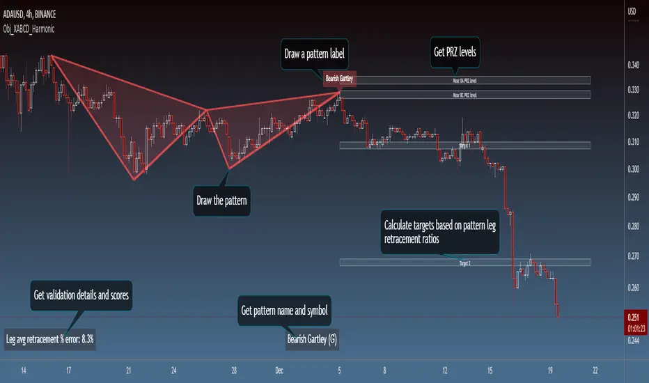
SnakeBand█ Overview.
This indicator is based on a calculation method made using a ichimoku and Fibonacci.
There are two lines, the upper line is the upper limit and the lower line is the lower limit.
These upper and lower limits are drawn ahead of 26 candles, just like Ichimoku.
█ Role.
The characteristic of this indicator is that
When prices reach the upper limit, they usually hesitate or try to fall, and when they reach the lower limit, they usually rebound or hesitate.
In particular, it has an excellent effect on low-point purchases.
Of course, it is often not the case, so you have to observe the speed and movement of the decline carefully, and it can be more effective if applied with the Elliot wave or harmonic.
It can also be more effective if used with rsi or macd bowling bands.
█ Memo.
It applies to all four-hour bong, three-hour bong, one-bong, and main bong.
It is important to keep studying and observing. This can give you the ability to capture the upward transition after hitting the lower limit.

eHarmonicpatternsExtendedLibrary "eHarmonicpatternsExtended"
Library provides an alternative method to scan harmonic patterns. This is helpful in reducing iterations. Republishing as new library instead of existing eHarmonicpatterns because I need that copy for existing scripts.
scan_xab(bcdRatio, err_min, err_max, patternArray) Checks if bcd ratio is in range of any harmonic pattern
Parameters:
bcdRatio : AB/XA ratio
err_min : minimum error threshold
err_max : maximum error threshold
patternArray : Array containing pattern check flags. Checks are made only if flags are true. Upon check flgs are overwritten.
scan_abc_axc(abcRatio, axcRatio, err_min, err_max, patternArray) Checks if abc or axc ratio is in range of any harmonic pattern
Parameters:
abcRatio : BC/AB ratio
axcRatio : XC/AX ratio
err_min : minimum error threshold
err_max : maximum error threshold
patternArray : Array containing pattern check flags. Checks are made only if flags are true. Upon check flgs are overwritten.
scan_bcd(bcdRatio, err_min, err_max, patternArray) Checks if bcd ratio is in range of any harmonic pattern
Parameters:
bcdRatio : CD/BC ratio
err_min : minimum error threshold
err_max : maximum error threshold
patternArray : Array containing pattern check flags. Checks are made only if flags are true. Upon check flgs are overwritten.
scan_xad_xcd(xadRatio, xcdRatio, err_min, err_max, patternArray) Checks if xad or xcd ratio is in range of any harmonic pattern
Parameters:
xadRatio : AD/XA ratio
xcdRatio : CD/XC ratio
err_min : minimum error threshold
err_max : maximum error threshold
patternArray : Array containing pattern check flags. Checks are made only if flags are true. Upon check flgs are overwritten.
isHarmonicPattern(x, a, b, c, d, flags, errorPercent) Checks for harmonic patterns
Parameters:
x : X coordinate value
a : A coordinate value
b : B coordinate value
c : C coordinate value
d : D coordinate value
flags : flags to check patterns. Send empty array to enable all
errorPercent : Error threshold
Returns: Array of boolean values which says whether valid pattern exist and array of corresponding pattern names
isHarmonicProjection(x, a, b, c, flags, errorPercent) Checks for harmonic pattern projection
Parameters:
x : X coordinate value
a : A coordinate value
b : B coordinate value
c : C coordinate value
flags : flags to check patterns. Send empty array to enable all
errorPercent : Error threshold
Returns: Array of boolean values which says whether valid pattern exist and array of corresponding pattern names.
get_prz_range(x, a, b, c, patternArray, errorPercent, start_adj, end_adj) Provides PRZ range based on BCD and XAD ranges
Parameters:
x : X coordinate value
a : A coordinate value
b : B coordinate value
c : C coordinate value
patternArray : Pattern flags for which PRZ range needs to be calculated
errorPercent : Error threshold
start_adj : - Adjustments for entry levels
end_adj : - Adjustments for stop levels
Returns: Start and end of consolidated PRZ range
get_prz_range_xad(x, a, b, c, patternArray, errorPercent, start_adj, end_adj) Provides PRZ range based on XAD range only
Parameters:
x : X coordinate value
a : A coordinate value
b : B coordinate value
c : C coordinate value
patternArray : Pattern flags for which PRZ range needs to be calculated
errorPercent : Error threshold
start_adj : - Adjustments for entry levels
end_adj : - Adjustments for stop levels
Returns: Start and end of consolidated PRZ range
WAP Maverick - (Dual EMA Smoothed VWAP) - [mutantdog]Short Version:
This here is my take on the popular VWAP indicator with several novel features including:
Dual EMA smoothing.
Arithmetic and Harmonic Mean plots.
Custom Anchor feat. Intraday Session Sizes.
2 Pairs of Bands.
Side Input for Connection to other Indicator.
This can be used 'out of the box' as a replacement VWAP, benefitting from smoother transitions and easy-to-use custom alerts.
By design however, this is intended to be a highly customisable alternative with many adjustable parameters and a pseudo-modular input system to connect with another indicator. Well suited for the tweakers around here and those who like to get a little more creative.
I made this primarily for crypto although it should work for other markets. Default settings are best suited to 15m timeframe - the anchor of 1 week is ideal for crypto which often follows a cyclical nature from Monday through Sunday. In 15m, the default ema length of 21 means that the wap comes to match a standard vwap towards the end of Monday. If using higher chart timeframes, i recommend decreasing the ema length to closely match this principle (suggested: for 1h chart, try length = 8; for 4h chart, length = 2 or 3 should suffice).
Note: the use of harmonic mean calculations will cause problems on any data source incorporating both positive and negative values, it may also return unusable results on extremely low-value charts (eg: low-sat coins in /btc pairs).
Long version:
The development of this project was one driven more by experimentation than a specific end-goal, however i have tried to fine-tune everything into a coherent usable end-product. With that in mind then, this walkthrough will follow something of a development chronology as i dissect the various functions.
DUAL-EMA SMOOTHING
At its core this is based upon / adapted from the standard vwap indicator provided by TradingView although I have modified and changed most of it. The first mod is the dual ema smoothing. Rather than simply applying an ema to the output of the standard vwap function, instead i have incorporated the ema in a manner analogous to the way smas are used within a standard vwma. Sticking for now with the arithmetic mean, the basic vwap calculation is simply sum(source * volume) / sum(volume) across the anchored period. In this case i have simply applied an ema to each of the numerator and denominator values resulting in ema(sum(source * volume)) / ema(sum(volume)) with the ema length independent of the anchor. This results in smoother (albeit slower) transitions than the aforementioned post-vwap method. Furthermore in the case when anchor period is equal to current timeframe, the result is a basic volume-weighted ema.
The example below shows a standard vwap (1week anchor) in blue, a 21-ema applied to the vwap in purple and a dual-21-ema smoothed wap in gold. Notably both ema types come to effectively resemble the standard vwap after around 24 hours into the new anchor session but how they behave in the meantime is very different. The dual-ema transitions quite gradually while the post-vwap ema immediately sets about trying to catch up. Incidentally. a similar and slower variation of the dual-ema can be achieved with dual-rma although i have not included it in this indicator, attempted analogues using sma or wma were far less useful however.
STANDARD DEVIATION AND BANDS
With this updated calculation, a corresponding update to the standard deviation is also required. The vwap has its own anchored volume-weighted st.dev but this cannot be used in combination with the ema smoothing so instead it has been recalculated appropriately. There are two pairs of bands with separate multipliers (stepped to 0.1x) and in both cases high and low bands can be activated or deactivated individually. An example usage for this would be to create different upper and lower bands for profit and stoploss targets. Alerts can be set easily for different crossing conditions, more on this later.
Alongside the bands, i have also added the option to shift ('Deviate') the entire indicator up or down according to a multiple of the corrected st.dev value. This has many potential uses, for example if we want to bias our analysis in one direction it may be useful to move the wap in the opposite. Or if the asset is trading within a narrow range and we are waiting on a breakout, we could shift to the desired level and set alerts accordingly. The 'Deviate' parameter applies to the entire indicator including the bands which will remain centred on the main WAP.
CUSTOM (W)ANCHOR
Ever thought about using a vwap with anchor periods smaller than a day? Here you can do just that. I've removed the Earnings/Dividends/Splits options from the basic vwap and added an 'Intraday' option instead. When selected, a custom anchor length can be created as a multiple of minutes (default steps of 60 mins but can input any value from 0 - 1440). While this may not seem at first like a useful feature for anyone except hi-speed scalpers, this actually offers more interesting potential than it appears.
When set to 0 minutes the current timeframe is always used, turning this into the basic volume-weighted ema mentioned earlier. When using other low time frames the anchor can act as a pre-ema filter creating a stepped effect akin to an adaptive MA. Used in combination with the bands, the result is a kind of volume-weighted adaptive exponential bollinger band; if such a thing does not already exist then this is where you create it. Alternatively, by combining two instances you may find potential interesting crosses between an intraday wap and a standard timeframe wap. Below is an example set to intraday with 480 mins, 2x st.dev bands and ema length 21. Included for comparison in purple is a standard 21 ema.
I'm sure there are many potential uses to be found here, so be creative and please share anything you come up with in the comments.
ARITHMETIC AND HARMONIC MEAN CALCULATIONS
The standard vwap uses the arithmetic mean in its calculation. Indeed, most mean calculations tend to be arithmetic: sma being the most widely used example. When volume weighting is involved though this can lead to a slight bias in favour of upward moves over downward. While the effect of this is minor, over longer anchor periods it can become increasingly significant. The harmonic mean, on the other hand, has the opposite effect which results in a value that is always lower than the arithmetic mean. By viewing both arithmetic and harmonic waps together, the extent to which they diverge from each other can be used as a visual reference of how much price has changed during the anchored period.
Furthermore, the harmonic mean may actually be the more appropriate one to use during downtrends or bearish periods, in principle at least. Consider that a short trade is functionally the same as a long trade on the inverse of the pair (eg: selling BTC/USD is the same as buying USD/BTC). With the harmonic mean being an inverse of the arithmetic then, it makes sense to use it instead. To illustrate this below is a snapshot of LUNA/USDT on the left with its inverse 1/(LUNA/USDT) = USDT/LUNA on the right. On both charts is a wap with identical settings, note the resistance on the left and its corresponding support on the right. It should be easy from this to see that the lower harmonic wap on the left corresponds to the upper arithmetic wap on the right. Thus, it would appear that the harmonic mean should be used in a downtrend. In principle, at least...
In reality though, it is not quite so black and white. Rarely are these values exact in their predictions and the sort of range one should allow for inaccuracies will likely be greater than the difference between these two means. Furthermore, the ema smoothing has already introduced some lag and thus additional inaccuracies. Nevertheless, the symmetry warrants its inclusion.
SIDE INPUT & ALERTS
Finally we move on to the pseudo-modular component here. While TradingView allows some interoperability between indicators, it is limited to just one connection. Any attempt to use multiple source inputs will remove this functionality completely. The workaround here is to instead use custom 'string' input menus for additional sources, preserving this function in the sole 'source' input. In this case, since the wap itself is dependant only price and volume, i have repurposed the full 'source' into the second 'side' input. This allows for a separate indicator to interact with this one that can be used for triggering alerts. You could even use another instance of this one (there is a hidden wap:mid plot intended for this use which is the midpoint between both means). Note that deleting a connected indicator may result in the deletion of those connected to it.
Preset alertconditions are available for crossings of the side input above and below the main wap, alongside several customisable alerts with corresponding visual markers based upon selectable conditions. Alerts for band crossings apply only to those that are active and only crossings of the type specified within the 'crosses' subsection of the indicator settings. The included options make it easy to create buy alerts specific to certain bands with sell alerts specific to other bands. The chart below shows two instances with differing anchor periods, both are connected with buy and sell alerts enabled for visible bands.
Okay... So that just about covers it here, i think. As mentioned earlier this is the product of various experiments while i have been learning my way around PineScript. Some of those experiments have been branched off from this in order to not over-clutter it with functions. The pseudo-modular design and the 'side' input are the result of an attempt to create a connective framework across various projects. Even on its own though, this should offer plenty of tweaking potential for anyone who likes to venture away from the usual standards, all the while still retaining its core purpose as a traders tool.
Thanks for checking this out. I look forward to any feedback below.
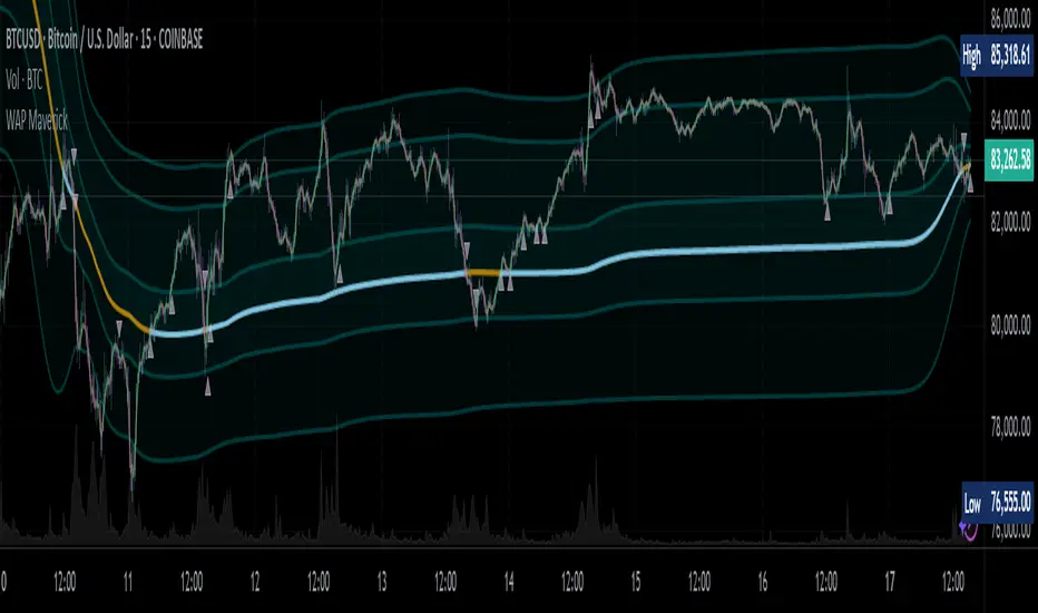
eHarmonicpatternsLibrary "eHarmonicpatterns"
Library provides an alternative method to scan harmonic patterns. This is helpful in reducing iterations
scan_xab(bcdRatio, err_min, err_max, patternArray) Checks if bcd ratio is in range of any harmonic pattern
Parameters:
bcdRatio : AB/XA ratio
err_min : minimum error threshold
err_max : maximum error threshold
patternArray : Array containing pattern check flags. Checks are made only if flags are true. Upon check flgs are overwritten.
scan_abc_axc(abcRatio, axcRatio, err_min, err_max, patternArray) Checks if abc or axc ratio is in range of any harmonic pattern
Parameters:
abcRatio : BC/AB ratio
axcRatio : XC/AX ratio
err_min : minimum error threshold
err_max : maximum error threshold
patternArray : Array containing pattern check flags. Checks are made only if flags are true. Upon check flgs are overwritten.
scan_bcd(bcdRatio, err_min, err_max, patternArray) Checks if bcd ratio is in range of any harmonic pattern
Parameters:
bcdRatio : CD/BC ratio
err_min : minimum error threshold
err_max : maximum error threshold
patternArray : Array containing pattern check flags. Checks are made only if flags are true. Upon check flgs are overwritten.
scan_xad_xcd(xadRatio, xcdRatio, err_min, err_max, patternArray) Checks if xad or xcd ratio is in range of any harmonic pattern
Parameters:
xadRatio : AD/XA ratio
xcdRatio : CD/XC ratio
err_min : minimum error threshold
err_max : maximum error threshold
patternArray : Array containing pattern check flags. Checks are made only if flags are true. Upon check flgs are overwritten.
isHarmonicPattern(x, a, c, c, d, flags, errorPercent) Checks for harmonic patterns
Parameters:
x : X coordinate value
a : A coordinate value
c : B coordinate value
c : C coordinate value
d : D coordinate value
flags : flags to check patterns. Send empty array to enable all
errorPercent : Error threshold
Returns: Array of boolean values which says whether valid pattern exist and array of corresponding pattern names
isHarmonicProjection(x, a, c, c, flags, errorPercent) Checks for harmonic pattern projection
Parameters:
x : X coordinate value
a : A coordinate value
c : B coordinate value
c : C coordinate value
flags : flags to check patterns. Send empty array to enable all
errorPercent : Error threshold
Returns: Array of boolean values which says whether valid pattern exist and array of corresponding pattern names

Signal_Data_2021_09_09__2021_11_18Library "Signal_Data_2021_09_09__2021_11_18"
Functions to support my timing signals system
import_start_time(harmonic) get the start time for each harmonic signal
Parameters:
harmonic : is an integer identifying the harmonic
Returns: the starting timestamp of the harmonic data
import_signal(index, harmonic) access point for pre-processed data imported here by copy paste
Parameters:
index : is the current data index, use 0 to initialize
harmonic : is the data set to index, use 0 to initialize
Returns: the data from the indicated harmonic array starting at index, and the starting timestamp of that data
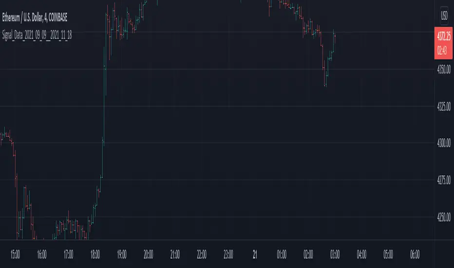
AB=CD Pattern Educational (Source Code)This indicator was intended as educational purpose only for AB=CD Patterns.
AB=CD Patterns were explained and modernized starting from The Harmonic Trader and Harmonic Trading: Volume One until Volume Three written by Scott M Carney.
Indikator ini bertujuan sebagai pendidikan sahaja untuk AB=CD Pattern.
AB=CD Patterns telah diterangkan dan dimodenkan bermula dari The Harmonic Trader dan Harmonic Trading: Volume One hingga Volume Three ditulis oleh Scott M Carney.
Indicator features :
1. List AB=CD patterns including ratio and reference page.
2. For desktop display only, not for mobile.
Kemampuan indikator :
1. Senarai AB=CD pattern termasuk ratio and rujukan muka surat.
2. Untuk paparan desktop sahaja, bukan untuk mobile.
FAQ
1. Credits / Kredit
Scott M Carney
Scott M Carney, Harmonic Trading: Volume One until Volume Three
2. Pattern and Chapter involved / Pattern dan Bab terlibat
Ideal AB=CD - The Harmonic Trader - Page 118 & 129
Standard AB=CD - The Harmonic Trader - Page 116, 117, 127 & 128, Harmonic Trading: Volume One - Page 42, 51, Harmonic Trading: Volume Three - Page 76 & 78
Alternate AB=CD - The Harmonic Trader - Page 142 & 145, Harmonic Trading: Volume One - Page 62, 63
Perfect AB=CD - Harmonic Trading: Volume One - Page 64 & 66
Reciprocal AB=CD - Harmonic Trading: Volume Two - Page 74 & 76
AB=CD with ab=cd - The Harmonic Trader - Page 149 & 153
AB=CD with BC Layering Technique - Harmonic Trading: Volume Three - Page 81 & 84
3. Code Usage / Penggunaan Kod
Free to use for personal usage but credits are most welcomed especially for credits to Scott M Carney.
Bebas untuk kegunaan peribadi tetapi kredit adalah amat dialu-alukan terutamanya kredit kepada Scott M Carney.
Bullish / Bearish Ideal AB=CD
Bullish / Bearish Standard AB=CD
Bullish / Bearish Alternate AB=CD
Bullish / Bearish Perfect AB=CD
Bullish / Bearish Reciprocal AB=CD (Additional value for reciprocal retracement 3.140 and 3.618)
Bullish / Bearish AB=CD with ab=cd
Bullish / Bearish AB=CD with BC Layering Technique
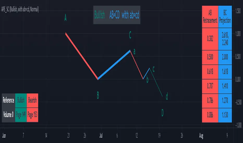
Bat Action Magnet Move BAMM Theory Educational (Source Code)This indicator was intended as educational purpose only for BAMM, which also known as Bat Action Magnet Move.
Indikator ini bertujuan sebagai pendidikan sahaja untuk BAMM, juga dikenali sebagai Bat Action Magnet Move.
BAMM is usually used for Harmonic Patterns such as XAB=CD (Bat Pattern) and AB=CD (0.5 AB=CD Pattern) - Chapter 5.
BAMM also can be used for other Harmonic Pattern with the help of RSI Divergence, hence become RSI BAMM - Chapter 6.
BAMM kebiasaanya digunakan untuk Harmonic Pattern seperti XAB=CD (Bat Pattern) dan AB=CD (0.5 AB=CD Pattern) - Chapter 5.
BAMM juga boleh digunakan untuk Harmonic Pattern lain dengan bantuan RSI Divergence, menjadi RSI BAMM - Chapter 6.
FAQ
1. Credits / Kredit
Scott M Carney,
Scott M Carney, Harmonic Trading: Volume Two (Chapter 5 & Chapter 6)
Bullish XAB=CD BAMM Breakout - Page 144
Bearish XAB=CD BAMM Breakdown - Page 148
Bullish AB=CD BAMM Breakout - Page 153
Bearish AB=CD BAMM Breakdown - Page 156
2. Code Usage / Penggunaan Kod
Free to use for personal usage but credits are most welcomed especially for credits to Scott M Carney.
Bebas untuk kegunaan peribadi tetapi kredit adalah amat dialu-alukan terutamanya kredit kepada Scott M Carney.
2.0 AB=CD Pattern
XAB=CD Bat Pattern
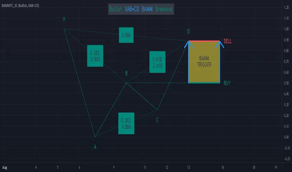
FIR Trend Filter (Sawtooth and Square Waves)Experimental script!
Using sigma approximation with Sine wave to form Sawtooth and Square waves, for a Finite Impulse Response filter.
Higher harmonics make the sawtooth or square wave more "exact", at the expense of more computation. It also makes the filter more "sensitive". I wouldn't exceed 100, but you're the boss.
The default number of harmonics is 20. The length is 20, too. Why? Because we are currently in 2020. Silly, I know.
Feel free to play around with the settings and tune it to your liking.
How to use it is pretty straight forward: Green is trend-up and red is trend-down.
Credit to alexgrover for the template.
