Momentum Breakout Filter + ATR ZonesMomentum Breakout Filter + ATR Zones - User Guide
What This Indicator Does
This indicator helps you with your MACD + volume momentum strategy by:
Filtering out fake breakouts - Shows ⚠️ warnings when breakouts lack confirmation
Showing clear entry signals - 🚀 LONG and 🔻 SHORT labels when all conditions align
Automatic stop loss & profit targets - Based on ATR (Average True Range)
Visual trend confirmation - Background color + EMA alignment
Signal Types
🚀 LONG Entry Signal (Green Label)
Appears when ALL conditions met:
✅ MACD crosses above signal line
✅ Volume > 1.5× average
✅ Price > EMA 9 > EMA 21 > EMA 200 (bullish trend)
✅ Price closes above recent 20-bar high
🔻 SHORT Entry Signal (Red Label)
Appears when ALL conditions met:
✅ MACD crosses below signal line
✅ Volume > 1.5× average
✅ Price < EMA 9 < EMA 21 < EMA 200 (bearish trend)
✅ Price closes below recent 20-bar low
⚠️ FAKE Breakout Warning (Orange Label)
Appears when price breaks high/low BUT lacks confirmation:
❌ Low volume (below 1.5× average), OR
❌ Wick break only (didn't close through level), OR
❌ MACD not aligned with direction
Hover over the warning label to see what's missing!
ATR Stop Loss & Targets
When you get a signal, colored lines automatically appear:
Long Position
Red solid line = Stop Loss (Entry - 1.5×ATR)
Green dashed lines = Profit Targets:
Target 1: Entry + 2×ATR
Target 2: Entry + 3×ATR
Target 3: Entry + 4×ATR
Short Position
Red solid line = Stop Loss (Entry + 1.5×ATR)
Green dashed lines = Profit Targets:
Target 1: Entry - 2×ATR
Target 2: Entry - 3×ATR
Target 3: Entry - 4×ATR
The lines move with each bar until you exit the position.
Chart Elements
Moving Averages
Blue line = EMA 9 (fast)
Orange line = EMA 21 (medium)
White line = EMA 200 (trend filter)
Volume
Yellow bars = High volume (above threshold)
Gray bars = Normal volume
Background Color
Light green = Bullish trend (all EMAs aligned up)
Light red = Bearish trend (all EMAs aligned down)
No color = Neutral/mixed
MACD (Bottom Pane)
Green/Red columns = MACD Histogram
Blue line = MACD Line
Orange line = Signal Line
Info Dashboard (Bottom Right)
ItemWhat It ShowsVolumeCurrent volume vs average (✓ HIGH or ✗ Low)MACDDirection (BULLISH or BEARISH)TrendEMA alignment (BULL, BEAR, or NEUTRAL)ATRCurrent ATR value in dollarsPositionCurrent position (LONG, SHORT, or NONE)R:RRisk-to-Reward ratio (shows when in position)
How To Use It
Basic Workflow
Wait for setup
Watch for MACD to approach signal line
Volume should be building
Price should be near EMA structure
Get confirmation
Wait for 🚀 LONG or 🔻 SHORT label
Check dashboard shows "✓ HIGH" volume
Verify trend is aligned (green or red background)
Enter the trade
Enter when signal appears
Note your stop loss (red line)
Note your targets (green dashed lines)
Manage the trade
Exit at first target for partial profit
Move stop to breakeven
Trail remaining position
What To Avoid
❌ Don't trade when you see:
⚠️ FAKE labels (wait for confirmation)
Neutral background (no clear trend)
"✗ Low" volume in dashboard
MACD and Trend not aligned
Settings You Can Adjust
Volume Sensitivity
High Volume Threshold: Default 1.5×
Increase to 2.0× for cleaner signals (fewer trades)
Decrease to 1.2× for more signals (more trades)
Fake Breakout Filters
You can toggle these ON/OFF:
Volume Confirmation: Requires high volume
Close Through: Requires candle close, not just wick
MACD Alignment: Requires MACD direction match
Tip: Turn all three ON for highest quality signals
ATR Stop/Target Multipliers
Default settings (conservative):
Stop Loss: 1.5×ATR
Target 1: 2×ATR (1.33:1 R:R)
Target 2: 3×ATR (2:1 R:R)
Target 3: 4×ATR (2.67:1 R:R)
Aggressive traders might use:
Stop Loss: 1.0×ATR
Target 1: 2×ATR (2:1 R:R)
Target 2: 4×ATR (4:1 R:R)
Conservative traders might use:
Stop Loss: 2.0×ATR
Target 1: 3×ATR (1.5:1 R:R)
Target 2: 5×ATR (2.5:1 R:R)
Example Trade Scenarios
Scenario 1: Perfect Long Setup ✅
Stock consolidating near EMA 21
MACD curling up toward signal line
Volume bar turns yellow (high volume)
🚀 LONG label appears
Red stop line and green target lines appear
Result: High probability trade
Scenario 2: Fake Breakout Avoided ✅
Price breaks above resistance
Volume is normal (gray bar)
⚠️ FAKE label appears (hover shows "Low volume")
No entry signal
Price falls back below breakout level
Result: Avoided losing trade
Scenario 3: Premature Entry ❌
MACD crosses up
Volume is high
BUT trend is NEUTRAL (no background color)
No signal appears (trend filter blocks it)
Result: Avoided choppy/sideways market
Quick Reference
Entry Checklist
🚀 or 🔻 label on chart
Dashboard shows "✓ HIGH" volume
Dashboard shows aligned MACD + Trend
Colored background (green or red)
ATR lines visible
No ⚠️ FAKE warning
Exit Strategy
Target 1 (2×ATR): Take 50% profit, move stop to breakeven
Target 2 (3×ATR): Take 25% profit, trail stop
Target 3 (4×ATR): Take remaining profit or trail aggressively
Stop Loss: Exit entire position if hit
Alerts
Set up these alerts:
Long Entry: Fires when 🚀 LONG signal appears
Short Entry: Fires when 🔻 SHORT signal appears
Fake Breakout Warning: Fires when ⚠️ appears (optional)
Tips for Success
Use on 5-minute charts for day trading momentum plays
Only trade high volume stocks ($5-20 range works best)
Wait for full confirmation - don't jump early
Respect the stop loss - it's calculated based on volatility
Scale out at targets - don't hold for home runs
Avoid trading first 15 minutes - let market settle
Best during 10am-11am and 2pm-3pm - peak momentum times
Common Questions
Q: Why didn't I get a signal even though MACD crossed?
A: All conditions must be met - check dashboard for what's missing (likely volume or trend alignment)
Q: Can I use this on any timeframe?
A: Yes, but it's designed for 5-15 minute charts. On daily charts, adjust ATR multipliers higher.
Q: The stop loss seems too tight, can I widen it?
A: Yes, increase "Stop Loss (×ATR)" from 1.5 to 2.0 or 2.5 in settings.
Q: I keep seeing FAKE warnings but price keeps going - what gives?
A: The filter is conservative. You can disable some filters in settings, but expect more false signals.
Q: Can I use this for swing trading?
A: Yes, but use larger timeframes (1H or 4H) and adjust ATR multipliers up (3× for stops, 6-9× for targets).
在脚本中搜索"stop loss"

Multi-Timeframe Trend Indicator with Signals═══════════════════════════════════════════════════════════════
Multi-Timeframe Trend Indicator with Signals
by Zakaria Safri
═══════════════════════════════════════════════════════════════
⚠️ IMPORTANT DISCLAIMERS:
━━━━━━━━━━━━━━━━━━━━━━━━━━━━━━━━━━━━━━━━━━━━━━━━━━━━━━━━━━━━━━
• This indicator may REPAINT on unconfirmed bars
• Signals appear in real-time but may change or disappear
• FOR EDUCATIONAL PURPOSES ONLY - NOT FINANCIAL ADVICE
• Past performance does not guarantee future results
• Always do your own research and use proper risk management
• The Risk Management feature is VISUAL ONLY - does not execute trades
━━━━━━━━━━━━━━━━━━━━━━━━━━━━━━━━━━━━━━━━━━━━━━━━━━━━━━━━━━━━━━
📊 OVERVIEW:
━━━━━━━━━━━━━━━━━━━━━━━━━━━━━━━━━━━━━━━━━━━━━━━━━━━━━━━━━━━━━━
This indicator combines multiple technical analysis tools to help identify
potential trend directions and entry/exit points across different timeframes.
It uses SuperTrend, EMAs, ADX, RSI, and Keltner Channels to generate signals.
🎯 KEY FEATURES:
━━━━━━━━━━━━━━━━━━━━━━━━━━━━━━━━━━━━━━━━━━━━━━━━━━━━━━━━━━━━━━
📍 SIGNAL TYPES:
• All Signals: Shows all SuperTrend crossovers
• Filtered Signals: Additional EMA filter for potentially higher quality signals
• Signals use barstate.isconfirmed to reduce (but not eliminate) repainting
📈 TREND ANALYSIS:
• Trend Ribbon: 8 EMAs creating a visual trend direction indicator
• Trend Cloud: EMA 150/250 cloud for long-term trend context
• Chaos Trend Line: Dynamic support/resistance trend line
• Multi-timeframe dashboard showing trend across 8 timeframes (3m to Daily)
📊 TECHNICAL INDICATORS:
• Keltner Channels: Dynamic price channels
• RSI Background: Visual overbought/oversold zones
• Candlestick Coloring: Three modes (CleanScalper/Trend Ribbon/Moving Average)
• ADX-based trend strength analysis for MTF dashboard
🎯 VISUAL TOOLS:
• Order Blocks: Supply/demand zones (optional)
• Channel Breakouts: Pivot-based support/resistance levels
• Reversal Signals: RSI-based potential reversal indicators
• Visual TP/SL Lines: For reference only - does NOT execute trades
📊 DASHBOARD:
• Real-time multi-timeframe trend analysis
• Volatility indicator (Very Low to Very High)
• Current RSI value with color coding
• Customizable position and size
⚙️ SETTINGS:
━━━━━━━━━━━━━━━━━━━━━━━━━━━━━━━━━━━━━━━━━━━━━━━━━━━━━━━━━━━━━━
MAIN SETTINGS:
• Sensitivity: Controls signal frequency (lower = more signals)
• Signal Type: Choose between All Signals or Filtered Signals
• Factor: ATR multiplier for SuperTrend calculation
TREND SETTINGS:
• Toggle Trend Ribbon, Trend Cloud, Chaos Trend, Order Blocks
• Moving Average: Customizable EMA (default 200)
ADVANCED SETTINGS:
• Candlestick coloring with 3 different modes
• Overbought/Oversold background coloring
• Channel breakout levels
• Show/hide signals
RISK MANAGEMENT (VISUAL ONLY):
• ⚠️ Does NOT execute trades automatically
• Shows potential Take Profit levels (TP1, TP2, TP3)
• Shows potential Stop Loss level
• Adjustable TP strength multiplier
• For educational reference only
📖 HOW TO USE:
━━━━━━━━━━━━━━━━━━━━━━━━━━━━━━━━━━━━━━━━━━━━━━━━━━━━━━━━━━━━━━
1. SIGNAL INTERPRETATION:
• "Buy" signals appear below candles when conditions are met
• "Sell" signals appear above candles when conditions are met
• Wait for bar close confirmation to avoid repainting
• Use multiple timeframes for confluence
2. TREND CONFIRMATION:
• Check the multi-timeframe dashboard for trend alignment
• Use Trend Ribbon for visual trend direction
• Trend Cloud shows longer-term market bias
• Green candles = potential uptrend, Red = potential downtrend
3. ENTRY/EXIT STRATEGY:
• Combine signals with other analysis tools
• Check volatility status before entering trades
• Use support/resistance levels for confirmation
• The visual TP/SL lines are for planning only
4. RISK MANAGEMENT:
• Always use stop losses (indicator shows suggested levels only)
• Position size according to your risk tolerance
• Never risk more than you can afford to lose
• The indicator does NOT manage trades automatically
⚠️ LIMITATIONS & RISKS:
━━━━━━━━━━━━━━━━━━━━━━━━━━━━━━━━━━━━━━━━━━━━━━━━━━━━━━━━━━━━━━
REPAINTING:
• Signals may appear and disappear on unconfirmed bars
• Always wait for bar close before taking action
• Historical performance may look better than real-time results
FALSE SIGNALS:
• No indicator is 100% accurate
• Signals can fail in ranging/choppy markets
• Use additional confirmation methods
• Consider market context and fundamentals
VISUAL TP/SL:
• Lines are for reference/planning only
• Does NOT place or manage actual trades
• You must manually set your own stop losses
• TP levels are calculated estimates, not guarantees
🔧 TECHNICAL DETAILS:
━━━━━━━━━━━━━━━━━━━━━━━━━━━━━━━━━━━━━━━━━━━━━━━━━━━━━━━━━━━━━━
• Version: Pine Script v5
• Overlay: Yes (displays on main chart)
• Anti-repaint measures: Uses barstate.isconfirmed on signals
• Security function: Uses lookahead protection for higher timeframes
• Dynamic requests: Enabled for MTF analysis
• Max labels: 500
📚 COMPONENTS EXPLAINED:
━━━━━━━━━━━━━━━━━━━━━━━━━━━━━━━━━━━━━━━━━━━━━━━━━━━━━━━━━━━━━━
SUPERTREND:
• Core signal generator using ATR-based bands
• Crossovers indicate potential trend changes
• Adjustable via Sensitivity and Factor inputs
EMA FILTER:
• Uses 200 EMA as trend filter (customizable)
• Filtered signals require price above/below EMA
• Helps reduce false signals in ranging markets
ADX TREND QUALITY:
• Measures trend strength across timeframes
• Used in multi-timeframe dashboard
• Shows Bullish/Bearish/Neutral states
KELTNER CHANNELS:
• Multiple bands showing volatility zones
• Color-coded based on RSI levels
• Helps identify overbought/oversold conditions
ORDER BLOCKS:
• Identifies supply/demand zones
• Based on price structure and pivots
• Can extend to the right for projection
💡 BEST PRACTICES:
━━━━━━━━━━━━━━━━━━━━━━━━━━━━━━━━━━━━━━━━━━━━━━━━━━━━━━━━━━━━━━
✓ Use multiple timeframe confirmation
✓ Wait for bar close before acting on signals
✓ Combine with support/resistance analysis
✓ Check overall market conditions
✓ Use proper risk management (1-2% per trade)
✓ Backtest on your specific market/timeframe
✓ Paper trade before using real money
✓ Keep a trading journal
✓ Adjust settings to your trading style
✗ Don't rely solely on this indicator
✗ Don't ignore risk management
✗ Don't trade on unconfirmed signals
✗ Don't overtrade every signal
✗ Don't use without understanding how it works
✗ Don't expect the TP/SL feature to trade for you
📞 SUPPORT & UPDATES:
━━━━━━━━━━━━━━━━━━━━━━━━━━━━━━━━━━━━━━━━━━━━━━━━━━━━━━━━━━━━━━
Creator: Zakaria Safri
Version: 4.3 (Compliance Update)
For questions or feedback, please use TradingView's comment section.
⚖️ FINAL DISCLAIMER:
━━━━━━━━━━━━━━━━━━━━━━━━━━━━━━━━━━━━━━━━━━━━━━━━━━━━━━━━━━━━━━
This indicator is provided for EDUCATIONAL and INFORMATIONAL purposes only.
It is NOT financial advice, investment advice, or a recommendation to buy/sell.
Trading involves substantial risk of loss. Past performance, whether actual or
indicated by historical tests of strategies, is not indicative of future results.
The creator assumes NO responsibility for your trading results. You are solely
responsible for your own investment decisions and due diligence.
Always consult with a qualified financial advisor before making investment decisions.
By using this indicator, you acknowledge and accept these risks and limitations.

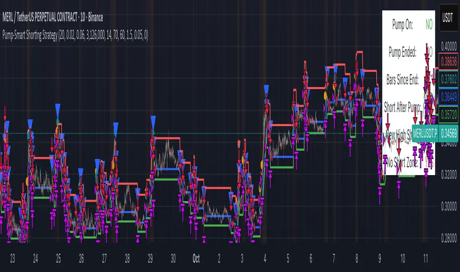
Pump-Smart Shorting StrategyThis strategy is built to keep your portfolio hedged as much as possible while maximizing profitability. Shorts are opened after pumps cool off and on new highs (when safe), and closed quickly during strong upward moves or if stop loss/profit targets are hit. It uses visual overlays to clearly show when hedging is on, off, or blocked due to momentum, ensuring you’re protected in most market conditions but never short against the pump. Fast re-entry keeps the hedge active with minimal downtime.
Pump Detection:
RSI (Relative Strength Index): Calculated over a custom period (default 14 bars). If RSI rises above a threshold (default 70), the strategy considers the market to be in a pump (strong upward momentum).
Volume Spike: The current volume is compared to a 20-bar simple moving average of volume. If it exceeds the average by 1.5× and price increases at least 5% in one bar, pump conditions are triggered.
Price Jump: Measured by (close - close ) / close . A single-bar change > 5% helps confirm rapid momentum.
Pump Zone (No Short): If any of these conditions is true, an orange or red background is shown and shorts are blocked.
Cooldown and Re-Entry:
Cooldown Detection: After the pump ends, RSI must fall below a set value (default ≤ 60), and either volume returns towards average or price momentum is less than half the original spike (oneBarUp <= pctUp/2).
barsWait Parameter: You can specify a waiting period after cooldown before a short is allowed.
Short Entry After Pump/Cooldown: When these cooldown conditions are met, and no short is active, a blue background is shown and a short position is opened at the next signal.
New High Entry:
Lookback New High: If the current high is greater than the highest high in the last N bars (default 20), and pump is NOT active, a short can be opened.
Take Profit (TP) & Stop Loss (SL):
Take Profit: Short is closed if price falls to a threshold below the entry (minProfitPerc, default 2%).
Stop Loss: Short is closed if price rises to a threshold above the entry (stopLossPerc, default 6%).
Preemptive Exit:
Any time a pump is detected while a short position is open, the strategy closes the short immediately to avoid losses.
Visual Feedback:
Orange Background: Market is pumping, do not short.
Red Background: Other conditions block shorts (cooldown or waiting).
Blue Background: Shorts allowed.
Triangles/Circles: Mark entries, pump start/end, for clear trading signals.
VMS Momentum Trend Matrix Indicator [09.00 to 23.30]VMS Momentum Trend Matrix Indicator - Detailed Explanation
🎯 Overview & Core Philosophy
This is a multi-dimensional trading and a multi-confirmation system that combines 4 independent analytical approaches into one unified framework. The indicator operates on the principle of "consensus trading" - where signals are only considered reliable when multiple systems confirm each other. The system is designed for 9:00 AM to 23:30 PM trading sessions (Indian Market) with dynamic support/resistance levels.
Five Pillars of Analysis:
1. Trend Matrix – Multiple indicator voting system
2. Momentum Suite – Multiple Hybrid oscillator
3. Volume Analysis - Buy/sell pressure quantification
4. Key Level Identification - Dynamic support/resistance
5. EMA Trend: Indicates the overall long-term direction.
📊 DASHBOARD INTERPRETATION - ROW BY ROW
ROW 1: Indicator Name and Cell background colour changes with Trend Matrix
ROW 2: EMA ANALYSIS (It analyses independently and does not combine this analysis with the Combined Analysis and Trading View. Background Colour on price chart is based on this)
Purpose: Long-term trend identification using Exponential Moving Averages
What to Watch:
• Major Trend: Overall market direction (Bullish/Bearish/Neutral)
• Bullish Condition: All EMAs aligned upward
• Bearish Condition: All EMAs aligned downward
• Neutral: Mixed alignment
Trading Significance:
• Trading Condition: Current bias based on EMA alignment
• Bullish Market: Focus on LONG positions only
• Bearish Market: Focus on SHORT positions only
• Neutral Market: Wait for clearer direction
ROW 3-4: KEY LEVELS
Purpose: Dynamic support and resistance identification
Levels to Monitor:
• VMS Line-1 (Support): Dynamic Support for long positions
• VMS Line-2 (Resistance): Dynamic Resistance for short positions
• Up/Down: Daily base levels from opening price calculations
• Up: Daily support level based on opening price
• Down: Daily resistance level based on opening price
How Levels Work:
• Wait for Line-1 and 2 Crossing
• In the Upward movement, Line-1 will move with the price, and Line-2 will be moved as a straight line
• In the Downward movement, Line-2 will move with the price, and Line-2 will be moved as a straight line
• Provide clear entry/exit points
• If the price is between these levels, it is mostly a sideways market. After the Upward movement, if the price crosses Line-1 and other bearish conditions are supported, a short position can be taken. And in the Downward movement, it is the reverse condition.
• If the price is above the up level, it can be considered as bullish and below as bearish
ROW 5-6: VOLUME ANALYSIS
Purpose: Measure buying vs selling pressure
Key Metrics:
• Total Buy Volume: Cumulative buying pressure
• Total Sell Volume: Cumulative selling pressure
• Bullish Candles: Number of up-candles in session
• Bearish Candles: Number of down-candles in session
Interpretation:
• Buy Volume > Sell Volume: Bullish sentiment
• Sell Volume > Buy Volume: Bearish sentiment
• Bullish Candles Dominating: Upward momentum
• Bearish Candles Dominating: Downward momentum
ROW 7-8: MOMENTUM SUITE (Background colour of Oscillator is based on this)
Purpose: Short-term momentum strength and direction
Critical Components:
• Direction: Current momentum (BULLISH/BEARISH)
• Strength: 0-100% strength measurement
• Bullish Height: Positive momentum magnitude
• Bearish Height: Negative momentum magnitude
Strength Classification:
• 80-100%: Very Strong - High conviction trades
• 60-80%: Strong - Good trading opportunities
• 40-60%: Moderate - Caution advised
• 20-40%: Weak - Avoid trading
• 0-20%: Very Weak - No trade zone
ROW 9-11: TREND MATRIX
Purpose: Consensus from Multiple technical indicators
Matrix Scoring:
• Bullish Signals: Number voting UP
• Bearish Signals: Number voting DOWN
• Neutral Signals: Non-committed indicators
• Net Score: Bullish - Bearish signals
Trend Classification:
• Strong Uptrend: Net Score ≥ +5
• Uptrend: Net Score +1 to +4
• Neutral: Net Score = 0
• Downtrend: Net Score -1 to -4
• Strong Downtrend: Net Score ≤ -5
ROW 12: COMBINED ANALYSIS
Purpose: Final integrated signal from all systems
Bias Levels:
• STRONG BULLISH: All systems aligned upward
• BULLISH: Majority systems upward
• NEUTRAL: Mixed or weak signals
• BEARISH: Majority systems downward
• STRONG BEARISH: All systems aligned downward
Confidence Score: 0-100% reliability measurement
ROW 13: TRADING VIEW
Purpose: Clear action recommendations
Possible Actions:
• STRONG LONG: High conviction buy signal
• MODERATE LONG: Medium conviction buy signal
• WAIT FOR CONFIRMATION: No clear signal
• MODERATE SHORT: Medium conviction sell signal
• STRONG SHORT: High conviction sell signal
🎯 COMPLETE TRADING RULES
BUY ENTRY CONDITIONS (All Must Be True)
Primary Conditions:
1. Combined Bias: BULLISH or STRONG BULLISH
2. Trading Action: MODERATE LONG or STRONG LONG
3. Momentum Strength: ≥ 40% (≥60% for STRONG LONG)
4. Trend Matrix: Net Score ≥ +3
5. EMA Trend: Bullish or Neutral
Confirmation Conditions:
6. Price Position: Above VMS Line-1 AND Base Up
7. Volume Confirmation: Buy Volume > Sell Volume
8. Bullish Candles: More bullish than bearish candles
Risk Management:
9. Stop Loss: Below VMS Line-1 OR Base Down (whichever is lower)
10. Position Size: Based on confidence score (higher score = larger position)
11. Take Profit: When Combined Bias turns "NEUTRAL" or momentum strength drops below 20%
12. Exit Signal: Trading Action shows "WAIT FOR CONFIRMATION"
SELL/SHORT ENTRY CONDITIONS (All Must Be True)
Primary Conditions:
1. Combined Bias: BEARISH or STRONG BEARISH
2. Trading Action: MODERATE SHORT or STRONG SHORT
3. Momentum Strength: ≥ 40% (≥60% for STRONG SHORT)
4. Bearish Signals: ≥ 12 in Trend Matrix
5. Trend Matrix: Net Score ≤ -3
6. EMA Trend: Bearish or Neutral
Confirmation Conditions:
6. Price Position: Below VMS Line-2 AND Base Down
7. Volume Confirmation: Sell Volume > Buy Volume
8. Bearish Candles: More bearish than bullish candles
Risk Management:
9. Stop Loss: Above VMS Line-2 OR Base Up (whichever is higher)
10. Position Size: Based on confidence score
11. Take Profit: When Combined Bias turns "NEUTRAL" or momentum strength drops below 20%
12. Exit Signal: Trading Action shows "WAIT FOR CONFIRMATION"
⏰ ENTRY/EXIT TIMING
Best Entry Times:
• 9:30-11:00 AM: Early session momentum established
• 12:30-16:30 AM: Mid-session confirmation
• 21:30-23:00 PM: closing session momentum shifts
Avoid Trading:
• First 15 minutes: Excessive volatility
• 12:00-18:00 PM: Low liquidity period
• After 22:00 PM: Session closing volatility
Exit Triggers:
Profit Taking:
• Target 1: 1:1 Risk-Reward (exit 50% position)
• Target 2: 1.5:1 Risk-Reward (exit remaining 50%)
• Trailing Stop: Move stop to breakeven after Target 1
Stop Loss Triggers:
• Price crosses opposite VMS line
• Combined Bias changes to NEUTRAL
• Momentum Strength drops below 20%
• Volume confirmation reverses
•
Emergency Exit:
• Trend Matrix Net Score reverses direction
• 6-EMA trend changes direction
• Key support/resistance breaks against position
📈 TRADING SCENARIOS
Scenario 1: STRONG BULLISH SETUP
- Combined Bias: STRONG BULLISH
- Trading Action: STRONG LONG
- Momentum Strength: 75%
- Trend Matrix: Net Score +8
- Price: Above VMS Line-1 and Base Up
- Volume: Strong buy volume dominance
ACTION: Enter LONG with full position size
STOP LOSS: Below VMS Line-1
TARGET: 1.5:1 Risk-Reward ratio
Scenario 2: MODERATE BEARISH SETUP
- Combined Bias: BEARISH
- Trading Action: MODERATE SHORT
- Momentum Strength: 55%
- Trend Matrix: Net Score -4
- Price: Below VMS Line-2 but above Base Down
- Volume: Moderate sell volume dominance
ACTION: Enter SHORT with half position size
STOP LOSS: Above VMS Line-2
TARGET: 1:1 Risk-Reward ratio
Scenario 3: NEUTRAL/WAIT SETUP
- Combined Bias: NEUTRAL
- Trading Action: WAIT FOR CONFIRMATION
- Momentum Strength: 35%
- Trend Matrix: Net Score 0
- Mixed volume signals
ACTION: NO TRADE - Wait for clearer signals
________________________________________
⚠️ RISK MANAGEMENT RULES
Position Sizing:
• STRONG Signals (80-100% confidence): 100% normal position
• MODERATE Signals (60-79% confidence): 50-75% position
• WEAK Signals (40-59% confidence): 25% position or avoid
• VERY WEAK (<40% confidence): NO TRADE
Daily Loss Limits:
• Maximum 2% capital loss per day
• Maximum 3 consecutive losing trades
• Stop trading after the daily limit is reached
Trade Management:
• Never move the stop loss against a position
• Take partial profits at predetermined levels
• Never average down losing positions
• Respect all exit signals immediately
________________________________________
🔄 SIGNAL CONFIRMATION PROCESS
Step 1: Trend Direction
Check EMA alignment and Combined Bias
Step 2: Momentum Strength
Verify Momentum Strength ≥ 40% and direction matches trend
Step 3: Volume Confirmation
Confirm volume supports the direction
Step 4: Matrix Consensus
Ensure Trend Matrix agrees (Net Score ≥ |3|)
Step 5: Price Position
Verify price is on the correct side of key levels
Step 6: Entry Execution
Enter on a pullback to support/resistance with a stop loss
________________________________________
This system works best when you wait for all conditions to align. Patience is key - only trade when all systems confirm the same direction with adequate strength. The multiple confirmation layers significantly increase the probability of success but reduce trading frequency.

Cnagda Pure Price ActionCnagda Pure Price Action (CPPA) indicator is a pure price action-based system designed to provide traders with real-time, dynamic analysis of the market. It automatically identifies key candles, support and resistance zones, and potential buy/sell signals by combining price, volume, and multiple popular trend indicators.
How Price Action & Volume Analysis Works
Silver Zone – Logic, Reason, and Trade Planning
Logic & Visualization:
The Silver Zone is created when the closing price is the lowest in the chosen window and volume is the highest in that window.
Visually, a large silver-colored box/rectangle appears on the chart.
Thick horizontal lines (top and bottom) are drawn at the high and low of that candle/bar, extending to the right.
Reasoning:
This combination typically occurs at strong “accumulation” or support areas:
Sellers push the price down to the lowest point, but aggressive buyers step in with high volume, absorbing supply.
Indicates potential exhaustion of selling and likely shift in market control to buyers.
How to Plan Trades Using Silver Zone:
Watch if price returns to the Silver Zone in the future: It often acts as powerful support.
Bullish entries (buys) can be planned when price tests or slightly pierces this zone, especially if new buy signals occur (like yellow/green candle labels).
Place your stop-loss below the bottom line of the Silver Zone.
Target: Look for the nearest resistance or opposing zone, or use indicator’s bullish label as confirmation.
Extra Tip:
Multiple touches of the Silver Zone reinforce its importance, but if price closes deeply below it with high volume, that’s a caution signal—support may be breaking.
Black Zone – Logic, Reason, and Trade Planning (as CPPA):
Logic & Visualization:
The Black Zone is created when the closing price is the highest in the chosen window and volume is the lowest in that window.
Visually, a large black-colored box/rectangle appears on the chart, along with thick horizontal lines at the top (high) and bottom (low) of the candle, extending to the right.
Reasoning:
This combination signals a strong “distribution” or resistance area:
Buyers push the price up to a local high, but low volume means there is not much follow-through or conviction in the move.
Often marks exhaustion where uptrend may pause or reverse, as sellers can soon step in.
How to Plan Trades Using Black Zone:
If price revisits the Black Zone in the future, it often acts as major resistance.
Bearish entries (sells) are considered when price is near, testing, or slightly above the Black Zone—especially if new sell signals appear (like blue/red candle labels).
Place your stop-loss just above the top line of the Black Zone.
Target: Nearest support zone (such as a Silver Zone) or next indicator’s bearish label.
Extra Tip:
Multiple touches of the Black Zone make it stronger, but if price closes far above with rising volume, be cautious—resistance might be breaking.
Support Line – Logic, Reason, and Trade Planning (as Cppa):
Logic & Visualization:
The Support Line is a dynamically drawn dashed line (usually blue) that marks key price levels where the market has previously shown significant buying interest.
The line is generated whenever a candle forms a high price with high volume (orange logic).
The script checks for historical pivot lows, past support zones, and even higher timeframe (HTF) supports, and then extends a blue dashed line from that price level to the right, labeling it (sometimes as “Prev Support Orange, HTF”).
Reasoning:
This line helps you visually identify where demand has been strong enough to hold price from falling further—essentially a floor in the market used by professional traders.
If price approaches or re-tests this line, there’s a good chance buyers will defend it again.
How to Plan Trades Using Support Line:
Watch for price to approach the Support Line during down moves. If you see a bullish candlestick pattern, buy labels (yellow/green), or other indicators aligning, this can be a high-probability entry zone.
Great for planning stop-loss for long trades: place stops just below this line.
Target: Next resistance zone, Black Zone, or the top of the last swing.
Extra Tip:
Multiple confirmations (support line + Silver Zone + bullish label) provide powerful entry signals.
If price closes strongly below the Support Line with volume, be cautious—support may be breaking, and a trend reversal or deeper correction could follow.
Resistance Line – Logic, Reason, and Trade Planning (from CPPA):
Logic & Visualization:
The Resistance Line is a dynamically drawn dashed line (usually purple or red) that identifies price levels where the market has previously faced significant selling pressure.
This line is created when a candle reaches a high price combined with high volume (orange logic), or from a historical pivot high/resistance,
The script also tracks higher timeframe (HTF) resistance lines, labeled as “Prev Resistance Orange, HTF,” and extends these dashed lines to the right across the chart.
Reasoning:
Resistance Lines are visual markers of “supply zones,” where buyers previously failed, and sellers took control.
If the price returns to this line later, sellers may get active again to defend this level, halting the uptrend.
How to Plan Trades Using Resistance Line:
Watch for price to approach the Resistance Line during up moves. If you see bearish candlestick patterns, sell labels (blue/red), or bearish indicator confirmation, this becomes a strong shorting opportunity.
Perfect for placing stop-loss in short trades—put your stop just above the Resistance Line.
Target: Next support zone (Silver Zone) or bottom of the last swing.
If the price breaks above with high volume, avoid shorting—resistance may be failing.
Extra Tip:
Multiple resistances (Resistance Line + Black Zone + bearish label) make short signals stronger.
Choppy movement around this line often signals indecision; wait for a clear rejection before entering trades.
Bullish / Bearish Label – Logic, Reason, and Trade Planning:
Logic & Visualization:
The indicator constantly calculates a "Bull Score" and a "Bear Score" based on several factors:
Trend direction from price slope
Confirmation by popular indicators (RSI, ADX, SAR, CMF, OBV, CCI, Bollinger Bands, TWAP)
Adaptive scoring (higher score for each bullish/bearish condition met)
If Bull Score > Bear Score, the chart displays a green "BULLISH" label (usually below the bar).
If Bear Score > Bull Score, the chart displays a red "BEARISH" label (usually above the bar).
If neither dominates, a "NEUTRAL" label appears.
Reasoning:
The labels summarize complex price action and indicator analysis into a simple, actionable sentiment cue:
Bullish: Majority of conditions indicate buying strength; trend is up.
Bearish: Majority signals show selling pressure; trend is down.
How to Use in Trade Planning:
Use the Bullish label as confirmation to enter or hold long (buy) positions, especially if near support/Silver Zone.
Use the Bearish label to enter/hold short (sell) positions, especially if near resistance/Black Zone.
For best results, combine with candle color, volume analysis, or other labels (yellow/green for buys, blue/red for sells).
Avoid trading against these labels unless you have strong confluence from zones/support levels.
Yellow Label (Buy Signal) – Logic, Reason & Trade Planning:
Logic & Visualization:
The yellow label appears below a candle (label.style_label_up, yloc.belowbar) and marks a potential buy signal.
Script conditions:
The candle must be a “yellow candle” (which means it’s at the local lowest close, not a high, with normal volume).
Volume is decreasing for 2 consecutive candles (current volume < previous volume, previous volume < second previous).
When these conditions are met, a yellow label is plotted below the candle.
Reasoning:
This scenario often marks the end of selling pressure and start of possible accumulation—buyers may be stepping in as sellers exhaust.
Decreasing volume during a local price low means selling is slowing, possibly hinting at a reversal.
How to Trade Using Yellow Label:
Entry: Consider buying at/just above the yellow-labeled candle’s close.
Stop-loss: A bit below the candle’s low (or Silver Zone line, if present).
Target: Next resistance level, Black Zone, or chart’s bullish label.
Extra Tip:
If the yellow label is found at/near a Silver Zone or Support Line, and trend is “Bullish,” the setup gets even stronger.
Avoid trading if overall indicator shows “Bearish.”
Green Label (Buy with Increasing Volume) – Logic, Reason & Trade Planning:
Logic & Visualization:
The green label is plotted below a candle (label.style_label_up, yloc.belowbar) and marks a strong buy signal.
Script conditions:
The candle must be a “yellow candle” (at the local lowest close, normal volume).
Volume is increasing for 2 consecutive candles (current volume > previous volume, previous volume > second previous).
When these conditions are met, a green label is plotted below the candle.
Reasoning:
This scenario signals that buyers are stepping in aggressively at a local price low—the end of a downtrend with strong, rising activity.
Increasing volume at a price low is a classic sign of accumulation, where institutions or large players may be buying.
How to Trade Using Green Label:
Entry: Consider buying at/just above the green-labeled candle’s close for a momentum-based reversal.
Stop-loss: Slightly below the candle’s low, or the Silver Zone/support line if present.
Target: Nearest resistance zone/Black Zone, indicator’s bullish label, or next swing high.
Extra Tip:
If the green label is near other supports (Silver Zone, Support Line), the setup is extra strong.
Use confirmation from Bullish labels or trend signals for best results.
Green label setups are suitable for quick, high momentum trades due to increasing volume
Blue Label (Sell Signal on Decreasing Volume) – Logic, Reason & Trade Planning:
Logic & Visualization:
The blue label is plotted above a candle (label.style_label_down, yloc.abovebar) as a potential sell signal.
Script conditions:
The candle is a “blue candle” (local highest close, but not also lowest, and volume is neither highest nor lowest).
Volume is decreasing over 2 consecutive candles (current volume < previous, previous < two ago).
When these match, a blue label appears above the candle.
Reasoning:
This typically signals buyer exhaustion at a local high: price has gone up, but volume is dropping, suggesting big players may not be buying any more at these levels.
The trend is losing strength, and a reversal or pullback is likely.
How to Trade Using Blue Label:
Entry: Look to sell at/just below the candle with the blue label.
Stop-loss: Just above the candle’s high (or above the Black Zone/resistance if present).
Target: Nearest support, Silver Zone, or a swing low.
Extra Tip:
Blue label signals are stronger if they appear near Black Zones or Resistance Lines, or when the general market label is "Bearish."
As with buy setups, always check for confirmation from trend or volume before trading aggressively.
Here’s a summary of all key chart labels, zones, and trading logic of your Price Action script:
Silver Zone: Powerful support zone. Created at lowest close + highest volume. Best for buy entries near its lines.
Black Zone: Strong resistance zone. Created at highest close + lowest volume. Ideal for short trades near its levels.
Support Line: Blue dashed line at historical demand; buyers defend here. Look for bullish setups when price approaches.
Resistance Line: Purple/red dashed line at supply; sellers defend here. Great for bearish setups when price nears.
Bullish/Bearish Labels: Summarize trend direction using price action + multiple indicator confirmations. Plan buys, holds on bullish; sells, shorts on bearish.
Yellow Label: Buy signal on decreasing volume and local price low. Entry above candle, stop below, target next resistance.
Green Label: Strong buy on increasing volume at a price low. Entry for momentum trade, stop below, target next zone.
Blue Label: Sell signal on dropping volume and local price high. Entry below candle, stop above, target next support.
Best Practices:
Always combine zone/label signals for higher probability trades.
Use stop-loss near zones/lines for risk management.
Prefer trading in the trend direction (bullish/bearish label agrees with your entry).
if Any Question, Suggestion Feel free to ask
Disclaimer:
All information provided by this indicator is for educational and analysis purposes only, and should not be considered financial advice.

VMS Momentum Trend Matrix Indicator [09.15 to 15.30]VMS Momentum Trend Matrix Indicator - Detailed Explanation
🎯 Overview & Core Philosophy
This is a multi-dimensional trading and a multi-confirmation system that combines 4 independent analytical approaches into one unified framework. The indicator operates on the principle of "consensus trading" - where signals are only considered reliable when multiple systems confirm each other. The system is designed for 9:15 AM to 3:30 PM trading sessions (Indian Market) with dynamic support/resistance levels.
Five Pillars of Analysis:
1. Trend Matrix – Multiple indicator voting system
2. Momentum Suite – Multiple Hybrid oscillator
3. Volume Analysis - Buy/sell pressure quantification
4. Key Level Identification - Dynamic support/resistance
5. EMA Trend: Indicates the overall long-term direction.
📊 DASHBOARD INTERPRETATION - ROW BY ROW
ROW 1: Indicator Name and Cell background colour changes with Trend Matrix
ROW 2: EMA ANALYSIS (It analyses independently and does not combine this analysis with the Combined Analysis and Trading View. Background Colour on price chart is based on this)
Purpose: Long-term trend identification using Exponential Moving Averages
What to Watch:
• Major Trend: Overall market direction (Bullish/Bearish/Neutral)
• Bullish Condition: All EMAs aligned upward
• Bearish Condition: All EMAs aligned downward
• Neutral: Mixed alignment
Trading Significance:
• Trading Condition: Current bias based on EMA alignment
• Bullish Market: Focus on LONG positions only
• Bearish Market: Focus on SHORT positions only
• Neutral Market: Wait for clearer direction
ROW 3-4: KEY LEVELS
Purpose: Dynamic support and resistance identification
Levels to Monitor:
• VMS Line-1 (Support): Dynamic Support for long positions
• VMS Line-2 (Resistance): Dynamic Resistance for short positions
• Up/Down: Daily base levels from opening price calculations
• Up: Daily support level based on opening price
• Down: Daily resistance level based on opening price
How Levels Work:
• Wait for Line-1 and 2 Crossing
• In the Upward movement, Line-1 will move with the price, and Line-2 will be moved as a straight line
• In the Downward movement, Line-2 will move with the price, and Line-2 will be moved as a straight line
• Provide clear entry/exit points
• If the price is between these levels, it is mostly a sideways market. After the Upward movement, if the price crosses Line-1 and other bearish conditions are supported, a short position can be taken. And in the Downward movement, it is the reverse condition.
• If the price is above the up level, it can be considered as bullish and below as bearish
ROW 5-6: VOLUME ANALYSIS
Purpose: Measure buying vs selling pressure
Key Metrics:
• Total Buy Volume: Cumulative buying pressure
• Total Sell Volume: Cumulative selling pressure
• Bullish Candles: Number of up-candles in session
• Bearish Candles: Number of down-candles in session
Interpretation:
• Buy Volume > Sell Volume: Bullish sentiment
• Sell Volume > Buy Volume: Bearish sentiment
• Bullish Candles Dominating: Upward momentum
• Bearish Candles Dominating: Downward momentum
ROW 7-8: MOMENTUM SUITE (Background colour of Oscillator is based on this)
Purpose: Short-term momentum strength and direction
Critical Components:
• Direction: Current momentum (BULLISH/BEARISH)
• Strength: 0-100% strength measurement
• Bullish Height: Positive momentum magnitude
• Bearish Height: Negative momentum magnitude
Strength Classification:
• 80-100%: Very Strong - High conviction trades
• 60-80%: Strong - Good trading opportunities
• 40-60%: Moderate - Caution advised
• 20-40%: Weak - Avoid trading
• 0-20%: Very Weak - No trade zone
ROW 9-11: TREND MATRIX
Purpose: Consensus from Multiple technical indicators
Matrix Scoring:
• Bullish Signals: Number voting UP
• Bearish Signals: Number voting DOWN
• Neutral Signals: Non-committed indicators
• Net Score: Bullish - Bearish signals
Trend Classification:
• Strong Uptrend: Net Score ≥ +5
• Uptrend: Net Score +1 to +4
• Neutral: Net Score = 0
• Downtrend: Net Score -1 to -4
• Strong Downtrend: Net Score ≤ -5
ROW 12: COMBINED ANALYSIS
Purpose: Final integrated signal from all systems
Bias Levels:
• STRONG BULLISH: All systems aligned upward
• BULLISH: Majority systems upward
• NEUTRAL: Mixed or weak signals
• BEARISH: Majority systems downward
• STRONG BEARISH: All systems aligned downward
Confidence Score: 0-100% reliability measurement
ROW 13: TRADING VIEW
Purpose: Clear action recommendations
Possible Actions:
• STRONG LONG: High conviction buy signal
• MODERATE LONG: Medium conviction buy signal
• WAIT FOR CONFIRMATION: No clear signal
• MODERATE SHORT: Medium conviction sell signal
• STRONG SHORT: High conviction sell signal
🎯 COMPLETE TRADING RULES
BUY ENTRY CONDITIONS (All Must Be True)
Primary Conditions:
1. Combined Bias: BULLISH or STRONG BULLISH
2. Trading Action: MODERATE LONG or STRONG LONG
3. Momentum Strength: ≥ 40% (≥60% for STRONG LONG)
4. Trend Matrix: Net Score ≥ +3
5. 6-EMA Trend: Bullish or Neutral
Confirmation Conditions:
6. Price Position: Above VMS Line-1 AND Base Up
7. Volume Confirmation: Buy Volume > Sell Volume
8. Bullish Candles: More bullish than bearish candles
Risk Management:
9. Stop Loss: Below VMS Line-1 OR Base Down (whichever is lower)
10. Position Size: Based on confidence score (higher score = larger position)
11. Take Profit: When Combined Bias turns "NEUTRAL" or momentum strength drops below 20%
12. Exit Signal: Trading Action shows "WAIT FOR CONFIRMATION"
SELL/SHORT ENTRY CONDITIONS (All Must Be True)
Primary Conditions:
1. Combined Bias: BEARISH or STRONG BEARISH
2. Trading Action: MODERATE SHORT or STRONG SHORT
3. Momentum Strength: ≥ 40% (≥60% for STRONG SHORT)
4. Bearish Signals: ≥ 12 in Trend Matrix
5. Trend Matrix: Net Score ≤ -3
6. EMA Trend: Bearish or Neutral
Confirmation Conditions:
6. Price Position: Below VMS Line-2 AND Base Down
7. Volume Confirmation: Sell Volume > Buy Volume
8. Bearish Candles: More bearish than bullish candles
Risk Management:
9. Stop Loss: Above VMS Line-2 OR Base Up (whichever is higher)
10. Position Size: Based on confidence score
11. Take Profit: When Combined Bias turns "NEUTRAL" or momentum strength drops below 20%
12. Exit Signal: Trading Action shows "WAIT FOR CONFIRMATION"
⏰ ENTRY/EXIT TIMING
Best Entry Times:
• 9:30-10:00 AM: Early session momentum established
• 11:00-11:30 AM: Mid-session confirmation
• 1:30-2:00 PM: Afternoon momentum shifts
Avoid Trading:
• First 15 minutes: Excessive volatility
• 12:00-1:00 PM: Low liquidity period
• After 3:00 PM: Session closing volatility
Exit Triggers:
Profit Taking:
• Target 1: 1:1 Risk-Reward (exit 50% position)
• Target 2: 1.5:1 Risk-Reward (exit remaining 50%)
• Trailing Stop: Move stop to breakeven after Target 1
Stop Loss Triggers:
• Price crosses opposite VMS line
• Combined Bias changes to NEUTRAL
• Momentum Strength drops below 20%
• Volume confirmation reverses
•
Emergency Exit:
• Trend Matrix Net Score reverses direction
• 6-EMA trend changes direction
• Key support/resistance breaks against position
📈 TRADING SCENARIOS
Scenario 1: STRONG BULLISH SETUP
- Combined Bias: STRONG BULLISH
- Trading Action: STRONG LONG
- Momentum Strength: 75%
- Trend Matrix: Net Score +8
- Price: Above VMS Line-1 and Base Up
- Volume: Strong buy volume dominance
ACTION: Enter LONG with full position size
STOP LOSS: Below VMS Line-1
TARGET: 1.5:1 Risk-Reward ratio
Scenario 2: MODERATE BEARISH SETUP
- Combined Bias: BEARISH
- Trading Action: MODERATE SHORT
- Momentum Strength: 55%
- Trend Matrix: Net Score -4
- Price: Below VMS Line-2 but above Base Down
- Volume: Moderate sell volume dominance
ACTION: Enter SHORT with half position size
STOP LOSS: Above VMS Line-2
TARGET: 1:1 Risk-Reward ratio
Scenario 3: NEUTRAL/WAIT SETUP
- Combined Bias: NEUTRAL
- Trading Action: WAIT FOR CONFIRMATION
- Momentum Strength: 35%
- Trend Matrix: Net Score 0
- Mixed volume signals
ACTION: NO TRADE - Wait for clearer signals
________________________________________
⚠️ RISK MANAGEMENT RULES
Position Sizing:
• STRONG Signals (80-100% confidence): 100% normal position
• MODERATE Signals (60-79% confidence): 50-75% position
• WEAK Signals (40-59% confidence): 25% position or avoid
• VERY WEAK (<40% confidence): NO TRADE
Daily Loss Limits:
• Maximum 2% capital loss per day
• Maximum 3 consecutive losing trades
• Stop trading after the daily limit is reached
Trade Management:
• Never move the stop loss against a position
• Take partial profits at predetermined levels
• Never average down losing positions
• Respect all exit signals immediately
________________________________________
🔄 SIGNAL CONFIRMATION PROCESS
Step 1: Trend Direction
Check EMA alignment and Combined Bias
Step 2: Momentum Strength
Verify Momentum Strength ≥ 40% and direction matches trend
Step 3: Volume Confirmation
Confirm volume supports the direction
Step 4: Matrix Consensus
Ensure Trend Matrix agrees (Net Score ≥ |3|)
Step 5: Price Position
Verify price is on the correct side of key levels
Step 6: Entry Execution
Enter on a pullback to support/resistance with a stop loss
________________________________________
This system works best when you wait for all conditions to align. Patience is key - only trade when all systems confirm the same direction with adequate strength. The multiple confirmation layers significantly increase the probability of success but reduce trading frequency.

AVGO Advanced Day Trading Strategy📈 Overview
The AVGO Advanced Day Trading Strategy is a comprehensive, multi-timeframe trading system designed for active day traders seeking consistent performance with robust risk management. Originally optimized for AVGO (Broadcom), this strategy adapts well to other liquid stocks and can be customized for various trading styles.
🎯 Key Features
Multiple Entry Methods
EMA Crossover: Classic trend-following signals using fast (9) and medium (16) EMAs
MACD + RSI Confluence: Momentum-based entries combining MACD crossovers with RSI positioning
Price Momentum: Consecutive price action patterns with EMA and RSI confirmation
Hybrid System: Advanced multi-trigger approach combining all methodologies
Advanced Technical Arsenal
When enabled, the strategy analyzes 8+ additional indicators for confluence:
Volume Price Trend (VPT): Measures volume-weighted price momentum
On-Balance Volume (OBV): Tracks cumulative volume flow
Accumulation/Distribution Line: Identifies institutional money flow
Williams %R: Momentum oscillator for entry timing
Rate of Change Suite: Multi-timeframe momentum analysis (5, 14, 18 periods)
Commodity Channel Index (CCI): Cyclical turning points
Average Directional Index (ADX): Trend strength measurement
Parabolic SAR: Dynamic support/resistance levels
🛡️ Risk Management System
Position Sizing
Risk-based position sizing (default 1% per trade)
Maximum position limits (default 25% of equity)
Daily loss limits with automatic position closure
Multiple Profit Targets
Target 1: 1.5% gain (50% position exit)
Target 2: 2.5% gain (30% position exit)
Target 3: 3.6% gain (20% position exit)
Configurable exit percentages and target levels
Stop Loss Protection
ATR-based or percentage-based stop losses
Optional trailing stops
Dynamic stop adjustment based on market volatility
📊 Technical Specifications
Primary Indicators
EMAs: 9 (Fast), 16 (Medium), 50 (Long)
VWAP: Volume-weighted average price filter
RSI: 6-period momentum oscillator
MACD: 8/13/5 configuration for faster signals
Volume Confirmation
Volume filter requiring 1.6x average volume
19-period volume moving average baseline
Optional volume confirmation bypass
Market Structure Analysis
Bollinger Bands (20-period, 2.0 multiplier)
Squeeze detection for breakout opportunities
Fractal and pivot point analysis
⏰ Trading Hours & Filters
Time Management
Configurable trading hours (default: 9:30 AM - 3:30 PM EST)
Weekend and holiday filtering
Session-based trade management
Market Condition Filters
Trend alignment requirements
VWAP positioning filters
Volatility-based entry conditions
📱 Visual Features
Information Dashboard
Real-time display of:
Current entry method and signals
Bullish/bearish signal counts
RSI and MACD status
Trend direction and strength
Position status and P&L
Volume and time filter status
Chart Visualization
EMA plots with customizable colors
Entry signal markers
Target and stop level lines
Background color coding for trends
Optional Bollinger Bands and SAR display
🔔 Alert System
Entry Alerts
Customizable alerts for long and short entries
Method-specific alert messages
Signal confluence notifications
Advanced Alerts
Strong confluence threshold alerts
Custom alert messages with signal counts
Risk management alerts
⚙️ Customization Options
Strategy Parameters
Enable/disable long or short trades
Adjustable risk parameters
Multiple entry method selection
Advanced indicator on/off toggle
Visual Customization
Color schemes for all indicators
Dashboard position and size options
Show/hide various chart elements
Background color preferences
📋 Default Settings
Initial Capital: $100,000
Commission: 0.1%
Default Position Size: 10% of equity
Risk Per Trade: 1.0%
RSI Length: 6 periods
MACD: 8/13/5 configuration
Stop Loss: 1.1% or ATR-based
🎯 Best Use Cases
Day Trading: Designed for intraday opportunities
Swing Trading: Adaptable for longer-term positions
Momentum Trading: Excellent for trending markets
Risk-Conscious Trading: Built-in risk management protocols
⚠️ Important Notes
Paper Trading Recommended: Test thoroughly before live trading
Market Conditions: Performance varies with market volatility
Customization: Adjust parameters based on your risk tolerance
Educational Purpose: Use as a learning tool and customize for your needs
🏆 Performance Features
Detailed performance metrics
Trade-by-trade analysis capability
Customizable risk/reward ratios
Comprehensive backtesting support
This strategy is for educational purposes. Past performance does not guarantee future results. Always practice proper risk management and consider your financial situation before trading.
Liquidity SweeperStrategy Overview
This Pine Script implements a Liquidity Sweep Trading Strategy, a sophisticated approach that capitalizes on market manipulation tactics commonly used by institutional traders. The strategy identifies when price "sweeps" above recent swing highs or below swing lows to trigger stop losses and grab liquidity, then quickly reverses direction - creating high-probability trading opportunities.
Core Concept: What is a Liquidity Sweep?
A liquidity sweep occurs when:
Price breaks above a swing high (or below a swing low) to trigger retail stop losses
Institutional players absorb this liquidity at favorable prices
Price quickly reverses back into the previous range
This creates a "fake breakout" or "stop hunt" pattern
The strategy exploits these manipulative moves by entering trades in the direction of the reversal.
How the Strategy Works
1. Swing Point Detection
Uses a lookback period (default: 20 bars) to identify significant swing highs and lows
Employs proper pivot point detection using ta.highestbars() and ta.lowestbars()
Only considers confirmed swing points (not just recent highs/lows)
2. Liquidity Sweep Identification
High Sweep (Short Setup):
Price moves above the last swing high (triggering buy stops)
Same bar closes back below the swing high (showing rejection)
Low Sweep (Long Setup):
Price moves below the last swing low (triggering sell stops)
Same bar closes back above the swing low (showing support)
3. Confirmation Process
Requires price to stay within the swept range for a specified number of bars (default: 3)
This confirms the sweep was genuine and not just normal volatility
Prevents false signals and improves trade quality
4. Entry Logic
Long Entries: Triggered after confirmed low sweeps
Short Entries: Triggered after confirmed high sweeps
5. Risk Management
Stop Loss: Placed at a multiple of ATR (default: 1.5x) from entry price
Take Profit: Risk/Reward ratio based (default: 2:1)
Position Sizing: 10% of equity per trade (configurable)
Red X-crosses: High sweeps detected
Green X-crosses: Low sweeps detected
Red triangles (down): Short entry signals
Green triangles (up): Long entry signals
Horizontal lines: Current swing high/low levels
Info label: Shows last detected swing levels
Optimal Conditions:
Timeframes: 1H, 4H, and Daily work best
Market Conditions: Ranging and trending markets both suitable
Volatility: Moderate to high volatility preferred
Session Times: Most effective during active trading sessions
Strengths:
✅ Exploits institutional manipulation tactics
✅ Clear entry/exit rules with defined risk
✅ Works across multiple asset classes
✅ Includes proper confirmation to reduce false signals
✅ Visual clarity for manual verification
✅ Reasonable risk/reward parameters
Limitations:
⚠️ Requires patience - not a high-frequency strategy
⚠️ Market dependent - fewer signals in low volatility periods
⚠️ Needs sufficient lookback data for swing identification
⚠️ May have drawdown periods during strong trending moves
⚠️ Requires understanding of market structure concepts
Best Practices for Users
Optimization Tips:
Adjust lookback period based on timeframe (shorter for lower TFs)
Test different confirmation periods for your market
Consider market session times when backtesting
Use alongside volume analysis for additional confirmation
Risk Management:
Never risk more than 2-3% per trade of total capital
Consider reducing position size during high-impact news
Monitor correlation if trading multiple pairs simultaneously
Use additional filters (trend, support/resistance) for confluence
Backtesting Recommendations:
Test on at least 6 months of historical data
Include different market conditions (trending, ranging, volatile)
Consider transaction costs and slippage in results
Forward test on demo before live implementation
Expected Results
Based on typical liquidity sweep strategy performance:
Disclaimer
This strategy is based on market structure analysis and institutional trading behavior patterns. Past performance doesn't guarantee future results. Users should:
Thoroughly backtest before live trading
Start with small position sizes
Understand the underlying concepts before implementation
Consider combining with other analysis methods
Always use proper risk management
The strategy works best when traders understand the psychological and structural elements of liquidity sweeps rather than just following signals blindly.
5m Exit AlertsThese can help a lot with Daytrading if you don't have a price target in mind when there's no clear resistance / support nearby, and you don't trust the market enough to hold it as a swing trade.
Keep in mind that its main purpose is to give you a "warning" that it might be good to look at your screen, instead of guaranteeing you "now is the best time to exit". You won't reach high winning stats by blindly following this alert.
"A Exit LONG":
(I'm using letters instead of numbers for all Exit alerts to make sure I don't accidentally confuse Enter and Exit alerts).
There are 4 conditions that might trigger it. The reasons show up in the exit alert message (unfortunately only as a number, since alert messages can't have "dynamic text" in TradingView), and can also be displayed as symbols in the chart (see image above - make sure to enable "Show Signals" in the indicator settings first though).
Here are the conditions sorted from best to worst:
Technical reversal: Bearish Hammer candle with Volume > 2 * avg volume (of last 30 candles), when 5m candle closed. Reversal very likely. This is usually the best time to take your gains for the rest of the day.
EMA 3/8 cross: standard 5m EMA 3/8 cross, indicating a trend reversal, or at least a pullback. Can also be helpful to detect double tops / double bottoms.
Trailing Stop Loss: Crossed below 30m EMA 8, 5m candle closed. This is a "fallback" alert in case EMA 3 was already below EMA 8 before you set up the alert. It's not unlikely that the stock might go further down to VWAP, so depending on the chart and market this might be a good opportunity to save the gains you have left.
"Final" Stop Loss: Crossed below VWAP. Usually not a good sign. If you entered around VWAP your losses shouldn't be big yet, but if you plan on holding the stock the Daily chart and market outlook should better be quite convincing, and you wouldn't have needed to use this alert in the first place.
Keep in mind these work of course best if you picked a "good" stock: clear movement, tidy price action, high volume. Otherwise alerts are more likely to be triggered redundantly.
Always consider how the market and stock looks like, then decide whether to exit or not! Usually it makes sense to wait a bit to see f. e. whether the stock bounces off the 30m EMA 8, and it's just a pullback.
"B Enter SHORT":
Similar, but for shorts...
"C 1m Scalp LONG" + "D 1m Scalp SHORT":
Simple Scalping alert for EMA 3/8 cross on a 1m chart - but without needing to use a 1m chart to set it up!
Unfortunately it's not as accurate as manually setting this alert up on a 1m chart. It might be an advantage though that it sometimes is triggered 1-2 min later, since this means there are less redundant triggerings.
It can be useful esp. on high momentum trades, but I honestly haven't used it in a looong while.
"X Candle Close":
same as in 5m Entry indicator: triggered when 5m candle is confirmed
"Z Trend Change: UP" + "Z Trend Change: DOWN":
This one is meant to be used only on SPY: It alerts you when SPY is changing its trending direction, which might mean entering or closing existing trades.
I have therefore set it up to never end (by setting it to "Once Per Bar Close" in the alert settings).
It's based on DMI positive or negative being > 25. I had it based on VWAP at the beginning, but there were days where it was triggered every 5 minutes...
More infos: www.reddit.com

Trend MasterOverview
The Strategy is a trend-following trading system designed for forex, stocks, or other markets on TradingView. It uses pivot points to identify support and resistance levels, combined with a 200-period Exponential Moving Average (EMA) to filter trades. The strategy enters long or short positions based on trend reversals during specific trading sessions (London or New York). It incorporates robust risk management, including position sizing based on risk percentage or fixed amount, trailing stop-losses, breakeven moves, and weekly/monthly profit/loss limits to prevent overtrading.
This script is ideal for traders who want a semi-automated approach with visual aids like colored session backgrounds, support/resistance lines, and a performance dashboard. It supports backtesting from a custom start date and can limit trades to one per session for discipline. Alerts are built-in for entries, exits, and stop-loss adjustments, making it compatible with automated trading bots.
Key Benefits:
Trend Reversal Detection: Spots higher highs/lows and lower highs/lows to confirm trend changes.
Session Filtering: Trades only during high-liquidity sessions to avoid choppy markets.
Risk Control: Automatically calculates position sizes to risk only a set percentage or dollar amount per trade.
Performance Tracking: Displays a table of weekly or monthly P&L (profit and loss) with color-coded heatmaps for easy review.
Customizable: Adjust trade direction, risk levels, take-profit ratios, and more via inputs.
The strategy uses a 1:1.2 risk-reward ratio by default but can be tweaked.
How It Works
Trend Identification:
The script calculates pivot highs and lows using left (4) and right (2) bars to detect swing points.
It identifies patterns like Higher Highs (HH), Higher Lows (HL), Lower Highs (LH), and Lower Lows (LL) to determine the trend direction (uptrend if above resistance, downtrend if below support).
Support (green dotted lines) and resistance (red dotted lines) are drawn dynamically and update on trend changes.
Bars are colored blue (uptrend) or black (downtrend) for visual clarity.
Entry Signals:
Long Entry: Price closes above the 200 EMA, trend shifts from down to up (e.g., breaking resistance), during an active session (London or NY), and no trade has been taken that session (if enabled).
Short Entry: Price closes below the 200 EMA, trend shifts from up to down (e.g., breaking support), during an active session, and no prior trade that session.
Trades can be restricted to "Long Only," "Short Only," or "Both."
Entries are filtered by a start date (e.g., from January 2022) and optional month-specific testing.
Position Sizing and Risk:
Risk per trade: Either a fixed dollar amount (e.g., $500) or percentage of equity (e.g., 1%).
Quantity is calculated as: Risk Amount / (Entry Price - Stop-Loss Price).
This ensures you never risk more than intended, regardless of market volatility.
Stop-Loss (SL) and Take-Profit (TP):
SL for Longs: Set below the recent support level, adjustable by a "reduce value" (e.g., tighten by 0-90%) and gap (e.g., add a buffer).
SL for Shorts: Set above the recent resistance level, with similar adjustments.
TP: Based on risk-reward ratio (default 1.2:1), so if SL is 100 pips away, TP is 120 pips in profit.
Visual boxes show SL (red) and TP (green) on the chart for the next 4 bars after entry.
Trade Management:
Trailing SL: Automatically moves SL to the new support (longs) or resistance (shorts) if it tightens the stop without increasing risk.
Breakeven Move: If enabled, SL moves to entry price once profit reaches a set ratio of initial risk (default 1:1). For example, if risk was 1%, SL moves to breakeven at 1% profit.
One Trade Per Session: Prevents multiple entries in the same London or NY session to avoid overtrading.
Sessions include optional weekend inclusion and are highlighted (blue for London, green for NY).
Risk Limits (Weekly/Monthly):
Monitors P&L for the current week or month.
Stops trading if losses hit a limit (e.g., -3%) or profits reach a target (e.g., +7%).
Resets at the start of each new week/month.
Alerts notify when limits are hit.
Exits:
Trades exit at TP, SL, or manually via alerts.
No time-based exits; relies on price action.
Performance Dashboard:
A customizable table (position, size, colors) shows P&L percentages for each week/month in a grid.
Rows = Years, Columns = Weeks (1-52) or Months (1-12).
Color scaling: Green for profits (darker for bigger wins), red for losses (darker for bigger losses).
Yearly totals in the last column.
Helps visualize strategy performance over time without manual calculations.
Input Parameters Explained
Here's a breakdown of the main inputs for easy customization:
Trade Direction: "Both" (default), "Long Only," or "Short Only" – Controls allowed trade types.
Test Only Selected Month: If true, backtests only the specified month from the start year.
Start Year/Month: Sets the backtest start date (default: Jan 2022).
Include Weekends: If true, sessions can include weekends (rarely useful for forex).
Only One Trade Per Session: Limits to one entry per London/NY session (default: true).
Risk Management Time Frame: "Weekly" or "Monthly" – For P&L limits.
Enable Limits: Toggle weekly/monthly stop trading on loss/profit thresholds.
Loss Limit (%)/Profit Target (%): Stops trading if P&L hits these (e.g., -3% loss or +7% profit).
London/New York Session: Enable/disable, with time ranges (e.g., London: 0800-1300 UTC).
Left/Right Bars: For pivot detection (default: 4 left, 2 right) – Higher values smooth signals.
Support/Resistance: Toggle lines, colors, style, width.
Change Bar Color: Colors bars based on trend.
TP RR: Take-profit risk-reward (default: 1.2).
Stoploss Reduce Value: Tightens SL (negative values widen it, 0-0.9 range).
Stoploss Gap: Adds a buffer to SL (e.g., 0.1% away from support).
Move to Breakeven: Enables SL move to entry at a profit ratio (default: true, 1:1).
Use Risk Amount $: If true, risks fixed $ (e.g., 500); else, % of equity (default: 1%).
EMA 3: The slow EMA period (default: 200) for trend filter.
Performance Display: Toggle table, location (e.g., Bottom Right), size, colors, scaling for heatmaps.
Setup and Usage Tips
Add to Chart: Copy the script into TradingView's Pine Editor, compile, and add to your chart.
Backtesting: Use the Strategy Tester tab. Adjust inputs and test on historical data.
Live Trading: Connect alerts to a broker or bot (e.g., via webhook). The script sends JSON-formatted alerts for entry, exit, SL moves, and limits.
Best Markets: Works well on crypto pairs like SOLUSD or RUNEUSD on 4H timeframes.
Risk Warning: This is not financial advice. Always use demo accounts first. Past performance doesn't guarantee future results. Commission is set to 0.05% by default – adjust for your broker.
Customization: Experiment with EMA length or RR ratio for your style.

- Trading Bot – Dynamic RSI (Professional) - Robot Strategy -1. General Concept and Philosophy
This strategy was designed for systematic traders and work especially well on short timeframes (1 to 5 minutes), who seek to capture trend reversal movements with a high degree of confirmation. The goal is not to follow the trend, but to identify precise entry points in oversold or overbought zones, and then to exit the position dynamically to adapt to changing market conditions.
The originality of Trading Bot Dynamic RSI lies not in a single indicator, but in the intelligent fusion of several concepts:
Dynamic RSI bands for both entries and exits .
A triple confirmation filter to secure trade entries.
A fully parameterizable design ready for automation .
2. Originality at the Core of the Strategy: Key Features
Dynamic Exits on RSI Bands: This is a main original feature of this script. Unlike traditional strategies that use fixed Take-Profits and Stop-Losses, this one uses an exit RSI band, calculated with parameters independent of the entry ones. This allows the strategy to:
Adapt to Volatility: In a volatile market, the exit band will move further away, allowing for the capture of larger moves. In a ranging market, it will tighten to secure smaller gains.
Optimize Profits: The exit occurs when momentum genuinely fades, not at an arbitrary price level, thus maximizing the potential of each trade.
Triple Confirmation Filter for Precise Entries: To avoid false signals, each entry is validated by the convergence of three distinct conditions:
The base signal is generated when the price reaches an overbought or oversold zone, materialized by an RSI band calculated directly on the chart.
The WaveTrend oscillator must also be in an extreme zone, confirming that the short-term momentum is ready for a reversal.
Finally, the StochRSI must validate that the RSI itself is in an overbought or oversold condition, adding an extra layer of security.
"Automation Ready" Design: The strategy was developed with automation in mind.
Customizable Alert Messages: All messages for entries and exits (Long/Short) can be formatted to be compatible with automated trade execution platforms.
Precise Capital Management: The position size calculation can be set as a fixed amount (e.g., 100 USDT), a percentage of the total capital, or of the available capital, and includes leverage. These parameters are crucial for a trading bot.
3. Detailed Operation
Entry Logic: A position is opened only if the following three conditions are met:
The market price touches (or closes below/above) the entry RSI band (lower for a buy, upper for a sell).
The WaveTrend indicator is in the oversold zone (for a buy) or overbought zone (for a sell).
The Stochastic RSI indicator is also in the oversold zone (for a buy) or overbought zone (for a sell).
The order is placed as a limit order on the RSI band, allowing for execution at the best possible price.
Exit Logic: The primary exit is dynamic.
For a Long position, the trade is closed when the price reaches the upper exit RSI band.
For a Short position, the trade is closed when the price reaches the lower exit RSI band.
Optionally, a percentage-based Stop-Loss and Take-Profit can be activated for more traditional risk management, although the dynamic exit is the recommended default mechanism.
4. Ease of Use and Customization
Despite its internal complexity, the strategy is designed to be user-friendly :
Clear Settings Panel: Parameters are grouped by function (Long Entry, Long Exit, Quantity, etc.), and each option comes with an explanatory tooltip.
Integrated Display: All key information (performance, current settings) is displayed in clean and discreet tables directly on the chart, allowing you to see at a glance how the strategy is configured.
Total Flexibility: Although default settings are provided, every parameter (RSI lengths, levels, filters) can be adjusted to optimize the strategy on any asset (cryptocurrencies, Forex, indices...) and any timeframe.
5. Detailed Guide to User Settings
A comprehensive set of parameters
To offer you complete control and maximum flexibility, the strategy exposes a comprehensive set of parameters. Here is an overview of what you can customize:
Trading Mode and Display
Trading Mode: Choose to enable only long positions ("Long Only"), only short positions ("Short Only"), or both simultaneously ("Long and Short").
Display: Manage the information panels on the chart. You can opt for a full display, a minimal window showing the profit, or hide all information for a clean chart.
Filters Smoothing (StochRSI K)
Filters Smoothing: This key parameter adjusts the smoothing of the Stochastic RSI. A lower value will make the filter more responsive, generating more signals. A higher value will make it smoother, generating fewer but potentially more reliable signals.
LONG Position Settings
Long Only mode
Entry: Define the RSI length and Oversold level that draw the lower band for long position entries.
Exit: Independently configure the RSI length and Overbought level that draw the upper band for the dynamic position exit.
Options: Optionally enable a percentage-based Take-Profit and/or Stop-Loss.
SHORT Position Settings
Short Only Mode
Entry: Define the RSI length and Overbought level for the upper entry band for short positions.
Exit: Independently configure the RSI length and Oversold level for the lower dynamic exit band.
Options: Just like for long positions, you can enable a percentage-based Take-Profit and/or Stop-Loss.
Quantity and Leverage
Quantity Type: Calculate your position size in three ways: as a fixed cash amount, as a percentage of available capital, or as a percentage of the total account balance.
Amount: Specify the dollar amount or percentage to commit per trade.
Leverage: Set the leverage to be applied. This is crucial for automation.
Backtest Period
Backtest Period: Enable this option to limit the strategy's calculations to a specific time period. This is a powerful tool for testing performance under particular market conditions.
Bot Alert Messages
Bot Alert Messages: This section is dedicated to automation. Customize the exact text messages that will be sent by TradingView alerts for each event (enter long, exit long, etc.).
Other Settings (Advanced - Optional)
Other Settings: This section allows experienced users to fine-tune the confirmation engine. You can adjust the parameters of the WaveTrend and Stochastic RSI oscillators in detail.
Spread Calculator (Informative Only)
Spread Calculator: This handy tool helps you estimate the actual fees of your exchange to run a much more realistic backtest. This panel has no impact on the trading logic itself.
Disclaimer
This strategy provides signals based on past market conditions. Past performance is not indicative of future results. Trading involves risk, and it is the responsibility of each user to manage their risk appropriately. It is strongly recommended to conduct thorough backtests and to understand the functioning of each parameter before using this strategy in live conditions or automating it. Take into account transaction fees, spread, and slippage, which can impact real results.

TrendPilot AI v2 — Adaptive Trend Day Trading StrategyOverview
TrendPilot AI v2 is a structured, rules-based day trading strategy that identifies and follows market momentum using a sophisticated blend of technical indicators. Optimized for 15-minute and higher timeframes on high market cap cryptocurrencies (AAVE, SOL, ETH, BCH, BTC) to minimize manipulation risks, it adapts to changing market conditions with dynamic risk management and controlled re-entry logic to maximize trend participation while minimizing noise.
Core Logic
Multiple EMA Trend Confirmation — Uses three Exponential Moving Averages (fast, medium, slow) to detect robust bullish, bearish, or neutral trends, ensuring trades align with the prevailing market direction.
ADX Momentum Filter — Employs an ADX-based filter to confirm strong trends, avoiding entries in choppy or low-momentum markets.
Smart Entry Filter — Optional ATR-based buffer (period 14, multiplier 1.5) around the fast EMA prevents entries at overextended prices, enhancing trade precision.
Flexible Exit System — Offers multiple exit options: fixed take-profit (default 1.7 offset), trend-reversal exits, or ATR-based trailing stops (period 14, multiplier 2.0), with secure modes requiring candle closes for confirmation to gain Max Profit.
Controlled Re-Entry Logic — Allows re-entries after take-profit or price-based stop-loss with configurable wait periods (default 6 bars), max attempts (default 2), and EMA touch requirements (fast, medium, or slow).
State-Aware Risk Management — Tracks trend states and recent exits to adapt entries, with daily trade limits (default 5 long/short) and loss cooldowns (default 2 stop-losses) for disciplined trading.
How to Use & Configuration
Markets & Timeframes
Works with high market cap cryptocurrencies (AAVE, SOL, ETH, BCH, BTC).
Optimized for intraday charts (15m–4h) but adaptable to higher timeframes (e.g., 1h, 4h).
Trade Direction Settings
Dual Trades — Trades both long and short, quickly re-aligning after trend reversals.
Long Only — Ignores bearish signals, ideal for bullish markets or strong uptrends.
Short Only — Ignores bullish signals, suited for bearish markets or downtrends.
Risk Management Settings
Stop Loss Types
Trend Reversal — Closes positions when an opposite trend signal is confirmed (default).
Fixed Offset — Static stop at 3.5 offset from entry price (adjustable).
ATR Based — Dynamic trailing stop using ATR (period 14, multiplier 2.0), adjusting to market volatility.
Secure SL Mode — Optional setting to trigger price-based stops only on candle closes, reducing false exits.
Maximum recommended risk per trade is 5–10% of account equity.
Trade size is configurable (default 20 units) to match individual risk appetite.
Take Profit Options
Fixed Offset — Predefined target at 1.7 offset from entry (adjustable, e.g., 2.5 for SOL).
Secure TP Mode — Exits only when a candle closes beyond the target, ensuring reliable profit capture.
Trend Reversal — Exits on opposite trend signals when fixed TP is disabled, ideal for riding longer trends.
Trade Management Controls
Smart Entry Filter — Optional ATR-based buffer (period 14, multiplier 1.5) prevents chasing overextended prices.
Max Re-Entries — Limits continuation trades per trend cycle (default 2).
Daily Trade Limits — Caps long/short trades per day (default 5 each) for disciplined trading.
Daily Loss Cooldown — Pauses trading after a set number of stop-losses (default 2) per day.
Max Bars in Trade — Closes positions after a set duration (default 1440 bars) to prevent stale trades.
Configuration Steps
Apply the strategy to your chosen symbol (e.g., AAVE/USDT, SOL/USDT) and timeframe (15m or higher).
Select Trade Direction mode (Dual, Long Only, or Short Only).
Set Stop Loss (Trend Reversal, Fixed Offset, or ATR Based) and Take Profit (fixed or trend-reversal).
Adjust Smart Entry Filter, Max Re-Entries, Daily Limits, and Loss Cooldown as needed.
Test across multiple market conditions using the performance panel (top-right, showing Total Trades, Wins, Losses, Win Rate).
Enables automated trading via webhook integration with platforms like Binance Futures.
Set up alerts for long/short entries (🟢 Long, 🔴 Short) and exits (🎯 Max TP, 🛑 Max SL, 🚨 Force Exit).
Backtesting Guidance
Use realistic commission (default 0.01%) and slippage (default 2 ticks) matching your broker and instrument.
Validate performance over long historical periods (e.g., 3–6 months) to ensure >100 trades across different market regimes.
Avoid curve-fitting by testing on multiple high market cap coins (AAVE, SOL, ETH, BCH, BTC) and avoiding over-optimization.
EMA and ATR parameters are set to balanced, industry-standard values for realistic backtesting.
Best Practices, Defaults & Disclaimer
Best Practices
Use consistent and conservative position sizing (default 20 units).
Match commission and slippage to your broker’s actual rates.
Enable secure TP/SL modes for entries and exits to reduce false signals.
Test across different symbols, timeframes, and market phases before live trading.
Keep parameters simple to avoid overfitting.
Default Settings (Recommended Starting Point)
Initial Capital: $10,000
Order Size: Fixed, 20 units
Commission: 0.01%
Slippage: 2 ticks
Take Profit Offset: 1.7 (adjustable, e.g., 2.5 for SOL)
Stop Loss Type: Trend Reversal (default), Fixed Offset (3.5), or ATR Based (period 14, multiplier 2.0)
Smart Entry Filter: ATR period 14, multiplier 1.5 (optional)
Max Re-Entries: 2 per trend cycle
Daily Trade Limits: 5 long, 5 short
Daily Loss Cooldown: 2 stop-losses
Max Bars in Trade: 1440 bars
Subscription Information
TrendPilot AI v2 is an invite-only strategy, accessible only to approved subscribers.
Benefits include full access to all features, priority support, and regular updates.
Access is limited to ensure a high-quality user experience.
Compliance Status
No functional warnings in the script.
The script uses closed candle logic, ensuring no repainting or lookahead issues.
Designed for realistic backtesting with a $10,000 account and sustainable risk (≤5–10% per trade).
Disclaimer
This strategy is intended for educational and analytical purposes only. Trading involves substantial risk, and past performance does not guarantee future results. You are solely responsible for your own trading decisions and risk management.
Developed by: TrendPilotAI Team
For questions, setup guidance, or enhancement suggestions, contact TrendPilotAI Team via TradingView.

Breakout Range Signal with Quality Analysis [Dova Lazarus]📌 Breakout Range Signal with Quality Analysis
🎓 Training-focused indicator for breakout logic, SL & TP behavior and signal quality assessment
🔷 PURPOSE
This tool identifies breakout candles from a calculated channel range and visually simulates entries, stop losses, and take profits, providing live and historical performance metrics.
⚙️ MAIN SETTINGS
1️⃣ Channel Setup
channel_length = 10 → how many candles are averaged to form channel boundaries
channel_multiplier = 0.0 → adds expansion above/below the base channel
channel_smoothing_type = SMA → smoothing method for high/low averaging
📊 The channel consists of two moving averages: one from highs, the other from lows. When expanded (via multiplier), it creates a buffer range for breakout validation.
2️⃣ Signal Detection
Body > Channel % = 50 → a breakout candle's body must exceed 150% of the channel width
Signal Mode:
• Weak → every valid breakout candle is highlighted
• Strong → only the first signal in a sequence is shown (helps reduce noise)
🟦 Bullish signals (blue):
• Candle opens inside the channel
• Closes above the channel
• Body is large enough
• Optional: confirms with trend (if enabled)
🟨 Bearish signals (yellow):
• Candle opens inside the channel
• Closes below the channel
• Body is large enough
• Optional: confirms with trend
3️⃣ Trend Filter (optional)
Enabled via checkbox
Uses a higher timeframe MA to filter signals
Bullish signals are allowed only if price is below the trend MA
Bearish signals only if price is above it
⏱️ trend_timeframe = 1D (typically set higher than the chart's timeframe)
🟢 Trend line is plotted if enabled
🎯 ENTRY, STOP LOSS & TAKE PROFIT LOGIC
SL and TP are based on channel width, not fixed pip/tick size:
📍 Entry Price = close of the breakout candle
🛑 Stop Loss:
• Bullish → below the lower channel border (minus offset)
• Bearish → above the upper channel border (plus offset)
🎯 Take Profit:
• Bullish → entry + channel width × profit multiplier
• Bearish → entry − channel width × profit multiplier
You can control:
Profit Target Multiplier (e.g., 1.0 → TP = 1×channel width)
Stop Loss Target Multiplier (e.g., 0.5 → SL = 0.5×channel width)
Signals to Show = how many historical SL/TP setups to display
📈 Lines and labels ("TP", "SL") are drawn on the chart for clarity.
🧪 QUALITY ANALYSIS MODULE
If enabled, the indicator will:
Track each new signal (entry, SL, TP)
Analyze outcomes:
• Win = TP hit before SL
• Loss = SL hit before TP
• Expired = signal unresolved after N bars
Display statistics in a table (top-right corner):
📋 Table fields:
✅ Overall win rate
📈 Bullish win rate
📉 Bearish win rate
🔢 Total signals
🕓 Pending (still active trades)
Maximum bars to wait for outcome is customizable (max_bars_to_analyze).
📐 VISUALIZATION TOOLS
TP / SL lines per signal
Labels “TP” and “SL”
Optional channel lines and trendline for better context
Colored bars for valid signals (blue/yellow)
📌 BEST USE CASES
Understand how breakout signals are formed
Learn SL/TP logic based on dynamic range
Test how volatility affects trade outcomes
Use as a visual simulation of trade behavior over time

Bear Market Defender [QuantraSystems]Bear Market Defender
A system to short Altcoins when BTC is ranging or falling - benefit from Altcoin bleed or collapse .
QuantraSystems guarantees that the information created and published within this document and on the TradingView platform is fully compliant with applicable regulations, does not constitute investment advice, and is not exclusively intended for qualified investors.
Important Note!
The system equity curve presented here has been generated as part of the process of testing and verifying the methodology behind this script.
Crucially, it was developed after the system was conceptualized, designed, and created, which helps to mitigate the risk of overfitting to historical data. In other words, the system was built for robustness, not for simply optimizing past performance.
This ensures that the system is less likely to degrade in performance over time, compared to hyper-optimized systems that are tailored to past data. No tweaks or optimizations were made to this system post-backtest.
Even More Important Note!!
The nature of markets is that they change quickly and unpredictably. Past performance does not guarantee future results - this is a fundamental rule in trading and investing.
While this system is designed with broad, flexible conditions to adapt quickly to a range of market environments, it is essential to understand that no assumptions should be made about future returns based on historical data. Markets are inherently uncertain, and this system - like all trading systems - cannot predict future outcomes.
INTRODUCTION TO THE STAR FRAMEWORK
The STAR Framework – an abbreviation for Strategic Trading with Adaptive Risk - is a bespoke portfolio-level infrastructure for dynamic, multi-asset crypto trading systems. It combines systematic position management, adaptive sizing, and “intra-system” diversification, all built on a rigorous foundation of Risk-based position sizing .
At its core, STAR is designed to facilitate:
Adaptive position sizing based on user-defined maximum portfolio risk
Capital allocation across multiple assets with dynamic weight adjustment
Execution-aware trading with robust fee and slippage adjustment
Realistic equity curve logic based on a compounding realized PnL and additive unrealized PnL
The STAR Framework is intended for use as both a standalone portfolio system or preferred as a modular component within a broader trading “global portfolio” - delivering a balance of robustness and scalability across strategy types, timeframes, and market regimes.
RISK ALLOCATION VIA "R" CALCULATIONS
The foundational concept behind STAR is the use of the R unit - a dynamic representation of risk per trade. R is defined by the distance between a trade's entry and its stoploss, making it an intuitive and universally adaptive sizing unit across any token, timeframe, or market.
Example: Suppose the entry price is $100, and the stoploss is $95. A $5 move against the position represents a 1R loss. A 15% price increase to $115 would equal a +3R gain.
This makes R-based systems highly flexible: the user defines the percentage of capital that is put at risk per R and all positions are scaled accordingly - whether the token is volatile, illiquid, or slow-moving.
R is an advantageous method for determine position sizing - instead of being tied to complex value at risk mechanisms with having layered exit criteria, or continuous volatility-based sizing criteria that need to be adjusted while in an open trade, R allows for very straightforward sizing, invalidation and especially risk control – which is the most fundamental.
REALIZED BALANCE, FEES & SLIPPAGE ACCOUNTING
All position sizing, risk metrics, and the base equity curve within STAR are calculated based on realized balance only .
This means:
No sizing adjustments are made based on unrealized profit and loss ✅
No active positions are included in the system's realized equity until fully closed ✅
Every trade is sized precisely according to current locked-in realized portfolio balance ✅
This creates the safest risk profile - especially when multiple trades are open. Unrealized gains are not used to inflate sizing, ensuring margin safety across all assets.
All calculations also incorporate slippage and fees, based on user-defined estimates – which can and should be based upon user-collected data - and updated frequently forwards in time. These are not cosmetic, or simply applied to the final equity curve - they are fully integrated into the dynamic position sizing and equity performance , ensuring:
Stoploss hits result in exactly a −1R loss, even after slippage and fees ✅
Winners are discounted based on realistic execution costs ✅
No trade is oversized due to unaccounted execution costs ✅
Example - Slippage in R Units:
Let R be defined as the distance from entry to stoploss.
Suppose that distance is $1, and the trade is closed at a win of +$2.
If execution slippage leads to a 50 cent worse entry and a 50 cent worse exit, you’ve lost $1 extra - which is an additional 1R in execution slippage. This makes the effective return 1.0R instead of the intended 2.0R.
This is equivalent to a slippage value of 50%.
Thus, slippage in STAR is tracked and modelled on an R-adjusted basis , enabling more accurate long-term performance modelling.
MULTI-ASSET, LONG/SHORT SUPPORT
STAR supports concurrent long and short positions across multiple tokens. This can sometimes result in partially hedged exposure - for example, being long one asset and short another.
This structure has key benefits:
Diversifies idiosyncratic risk by distributing exposure across multiple tokens
Allows simultaneous exploitation of relative strength and weakness
Reduces portfolio volatility via natural hedging during reduced trending periods
Even in a highly correlated market like crypto, short-term momentum behaviour often varies between tokens - making diversified, multi-directional exposure a strategic advantage .
EQUITY CURVE
The STAR framework only updates the underlying realized equity when a position is closed, and the trade outcome is known. This approach ensures:
True representation of actual capital available for trading
No exposure distortion due to unrealized gains
Risk remains tightly linked to realized results
This trade-to-trade basis for realized equity modelling eliminates the common pitfall of overallocation based on unrealized profits.
The visual equity curve represents an accurate visualization of the Total Equity however, which is equivalent to what would be the realized equity if all trades were closed on the prior bar close.
TIMEFRAME CONSIDERATIONS
Lower timeframes typically yield better performance for STAR due to:
Greater data density per day - more observations = better statistical inference
Faster compounding - more trades per week = faster capital rotation
However, lower timeframes also suffer from increased slippage and fees. STAR's execution-aware structure helps mitigate this, but users must still choose timeframes appropriate to their liquidity, costs, and operational availability.
INPUT OPTIONS
Fees (direct trading costs - the percentage of capital removed from the initial position size)
Slippage (execution delay, as a percentage. In practice, the fill price is often worse than the signal price. This directly affects R and hence position sizing)
Risk % ( Please note : this is the risk level if every position is opened at once. 5% risk for 5 assets is 1% risk per position)
System Start date
Float Precision value of displayed numbers
Table visualization - positioning and table sizes
Adjustable color options
VISUAL SIMPLICITY
To avoid usual unnecessary complexity and empower fast at-a-glance action taking, as well as enable mobile compatibility, only the most relevant information is presented.
This includes all information required to open positions in one table.
As well as a quick and straightforward overview for the system stats
Lastly, there is an optional table that can be enabled
displaying more detailed information if desired:
USAGE GUIDELINES
To use STAR effectively:
Input your average slippage and fees %
Input your maximum portfolio risk % (this controls overall leverage and is equivalent to the maximum loss that the allocation to STAR would bring if ALL positions are allocated AND hit their stop loss at the same time)
Wait for signal alerts with entry, stop, and size details
STAR will dynamically calculate sizing, risk exposure, and portfolio allocation on your behalf. Position multipliers, stop placement, and asset-specific risk are all embedded in the system logic.
Note: Leverage must be manually set to ISOLATED on your exchange platform to prevent unwanted position linking.
ABOUT THE BEAR MARKET DEFENDER STRATEGY
The first strategy to launch on the STAR Framework is the BEAR MARKET DEFENDER (BMD) - a fast-acting, trend following system based upon the Trend Titan NEUTRONSTAR. For the details of the logic behind NEUTRONSTAR, please refer to the methodology and trend aggregation section of the following indicator:
The BMD ’s short side exit calculation methodology is slightly improved compared to NEUTRONSTAR, to capture downtrends more consistently and also cut positions faster – which is crucial when considering general jump risk in the Crypto space.
Accordingly, the only focus of the BMD is to capture trends to the short side, providing the benefit of being in a spectrum from no correlation to being negatively correlated in risk and return behavior to classical Crypto long exposure.
More precisely, Crypto behavior showcases that when Bitcoin is in a ranging/mean reverting environment, most tokens that don’t fall into the “Blue-Chip” category tend to find themselves in a trend towards 0.
Typically during this period most Crypto portfolios suffer heavily due to a “Crypto-long” biased exposure.
The Bear Market Defender thrives in these chaotic, high volatility markets where most coins trend towards zero while the traditional Crypto long exposure is either flat or in a drawdown, therefore the BMD adds a source of uncorrelated risk and returns to hedge typical long exposure and bolster portfolio volatility.
Because of the BMD's short-only exposure, it will often suffer small losses during strong uptrends. During these periods, long exposure performs the best and the goal is to outperform the temporary underperformance in the BMD .
To take advantage of the abovementioned behavior of most tokens trending to zero, assets traded in the BMD are systematically updated on a quarterly basis with available liquidity being an important consideration for the tokens to be eligible for selection.
FINAL SUMMARY
The STAR Framework represents a new generation of portfolio grade trading infrastructure, built around disciplined execution, realized equity, and adaptive position sizing. It is designed to support any number of future methodologies - beginning with BMD .
The Bear Market Defender is here to hedge out commonly long biased portfolio allocations in the Crypto market, specializing in bringing uncorrelated returns during periods of sideways price action on Bitcoin, or whole-market downturns.
Together, STAR + BMD deliver a scalable, volatility tuned system that prioritizes capital preservation, signal accuracy, and adaptive risk allocation. Whether deployed standalone or within a broader portfolio, this framework is engineered for high performance, longevity, and adaptability in the ever-evolving crypto landscape.

Opening Range Breakout with John Wick + CDH/CDLOpening Range Breakout (ORB) De Luxe with John Wick Pattern - User Manual Table of Contents
1. Introduction
2. Key Features
3. Installation
4. Configuration Guide
5. Trading Signals
6. Pattern Recognition
7. Zone Trading
8. Alert Setup
9. Trading Strategies
10. Best Practices
11. Troubleshooting
________________________________________
1. Introduction The Opening Range Breakout (ORB) with John Wick indicator is a comprehensive trading tool designed for intraday and swing traders. It combines the classic Opening Range Breakout strategy with advanced candlestick pattern recognition, including the unique "John Wick" pattern. What is Opening Range Breakout? The Opening Range (OR) is the price range established during the first 15 minutes of a trading session. This range often acts as support and resistance for the remainder of the trading day. Breakouts above or below this range can signal strong directional moves. Key Concepts: • Opening Range High: The highest price during the first 15 minutes • Opening Range Low: The lowest price during the first 15 minutes • Breakout: Price movement above OR High (bullish) or below OR Low (bearish) • Pattern Zones: Areas around key levels where pattern recognition is most effective • PDH/PDL: Previous Day High and Previous Day Low - key reference levels from the prior trading day • CDH/CDL: Current Day High and Current Day Low - dynamically updating intraday extremes
________________________________________
2. Key Features Core Features: • Multi-Session Support: New York, London, Tokyo, Sydney, Frankfurt, and Custom sessions • Opening Range Visualization: Automatic OR High/Low detection and plotting • Pattern Recognition: Engulfing, Hammer/Shooting Star, Doji, and John Wick patterns • Zone Trading: Customizable zones around OR and PDH/PDL/CDH/CDL levels • Previous Day Levels: PDH (Previous Day High) and PDL (Previous Day Low) • Current Day Levels: CDH (Current Day High) and CDL (Current Day Low) - real-time tracking • Mid-Point Levels: Automatic calculation of OR mid-point • Real-Time Alerts: Breakout and pattern-based alerts • Multi-Timezone Support: Exchange or custom timezone selection Visual Features: • Dynamic color-coded levels • Triangle signals for breakouts • Pattern labels with clear identification • Information table with current session data • Fully customizable colors and styles
________________________________________
3. Installation Step 1: Add to Chart
4. Open TradingView and navigate to your desired chart
5. Click on "Indicators" (or press /)
6. Search for "Opening Range Breakout with John Wick"
7. Click to add the indicator to your chart Step 2: Initial Setup
8. The indicator will automatically detect your chart's timezone
9. Default session is set to "New York"
10. All features are enabled by default Recommended Timeframes: • Optimal: 1-minute to 15-minute charts • Suitable: Up to 1-hour charts • Not Recommended: Daily or higher timeframes
________________________________________
4. Configuration Guide Timezone Settings Use Exchange Timezone • Enabled (Default): Uses the exchange's native timezone • Disabled: Uses chart timezone or custom selection Timezone Selection Available when "Use Exchange Timezone" is disabled: • America/New_York • Europe/London • Europe/Amsterdam • Asia/Tokyo • Australia/Sydney Session Selection Trading Sessions • Sydney: 09:00-16:00 Sydney time • Tokyo: 09:00-15:00 Tokyo time • London: 08:00-16:30 London time • Frankfurt: 09:00-17:30 Frankfurt time • New York: 09:30-16:00 New York time • Custom: User-defined session • Previous Sessions: Shows multiple historical ORs Custom Session Settings • Custom Session Time: Define your own trading hours • Custom Session Name: Label for your custom session Display Options Line Settings • Line Width: 1-5 (Default: 2) • Line Style: Solid, Dashed, or Dotted • Show Current Only: Hide historical OR lines • Show Session Name: Display session label on chart Color Customization • OR Resistance (High): Default red • OR Support (Low): Default green • Session Colors: Unique color per session type • Zone Colors: Separate colors for OR and PDH/PDL zones Pattern Zone Settings Zone Configuration • Show Pattern Detection Zone: Enable/disable zones • OR Zone Size: Percentage of OR range (Default: 2%) • PDH/PDL Zone Size: Percentage of PDH-PDL range (Default: 1.5%) • CDH/CDL Zone Size: Percentage of CDH-CDL range (Default: 1.5%) • Show Zone Labels: Display zone boundary values • Only Detect Patterns in Zone: Limit pattern detection to zones Mid-Point Settings • Show Opening Range Mid-Point: Display OR midline • Mid-Point Color: Default gray • Mid-Point Style: Dotted, Dashed, or Solid • Show Mid-Point Label: Display midpoint value Previous Day Levels • Show Previous Day High/Low: Enable PDH/PDL lines • PDH/PDL Colors: Default yellow • PDH/PDL Line Style: Customizable style • Show PDH/PDL Labels: Display level values
Current Day Levels • Show Current Day High/Low: Enable CDH/CDL lines • CDH/CDL Colors: Default blue • CDH/CDL Line Style: Customizable style • Show CDH/CDL Labels: Display level values • Update Frequency: Real-time updates as new highs/lows are made
________________________________________
5. Trading Signals Signal Types
6. Breakout Signals • Bullish (Buy): Green triangle below candle when price breaks above OR High • Bearish (Sell): Red triangle above candle when price breaks below OR Low
7. Pattern-Enhanced Signals Signals are generated when breakouts occur WITH confirming patterns: • Stronger probability of follow-through • Reduced false breakouts • Better risk/reward setups Signal Configuration Alert Settings • Enable Alerts: Turn alerts on/off • Show Buy/Sell Signals: Visual signals on chart • Show Signal Text: Display "BUY"/"SELL" labels Pattern Filter Options • Use Candle Pattern Filter: Require patterns for signals • Pattern Combination Mode: o Any Pattern: Signal on any single pattern o Multiple Patterns: Require minimum pattern count o Specific Combo: Require specific pattern combinations
________________________________________
6. Pattern Recognition Supported Patterns
7. Engulfing Pattern • Bullish Engulfing: Large green candle completely engulfs previous red candle • Bearish Engulfing: Large red candle completely engulfs previous green candle • Label: "E"
8. Hammer/Shooting Star • Hammer: Small body at top, long lower wick (2x body size) • Shooting Star: Small body at bottom, long upper wick (2x body size) • Labels: "H" (Hammer), "S" (Shooting Star)
9. Doji Pattern • Definition: Open and close nearly equal (body < 10% of average) • Significance: Indecision, potential reversal • Label: "D"
10. John Wick Pattern (Unique Feature) • Bullish John Wick: o Opens below previous candle's low o 30-70% of body extends below previous low o Strong momentum indication • Bearish John Wick: o Opens above previous candle's high o 30-70% of body extends above previous high • Label: "JW" Pattern Visualization • Pattern Markers: Small circular labels with pattern abbreviations • Pattern Count: Number showing total patterns detected • Pattern Background: Optional highlighting (disabled by default) • Positioning: o Bullish patterns: Below candles at varying distances o Bearish patterns: Above candles at varying distances
________________________________________
7. Zone Trading Zone Concept Zones are buffer areas around key levels where price action and patterns are monitored more closely. Zone Types
8. Opening Range Zones • OR High Zone: Area around the OR High level • OR Low Zone: Area around the OR Low level • Purpose: Identify potential breakout or rejection areas
9. PDH/PDL Zones • PDH Zone: Area around Previous Day High • PDL Zone: Area around Previous Day Low • Purpose: Monitor reactions at key daily levels
10. CDH/CDL Zones • CDH Zone: Area around Current Day High • CDL Zone: Area around Current Day Low • Purpose: Track reactions at evolving intraday extremes • Dynamic Nature: These zones move as new highs/lows are established Zone Features • Visual Representation: Semi-transparent colored boxes • Customizable Size: Percentage-based calculation • Pattern Detection: Option to only detect patterns within zones • Bar Coloring: Candles change color when in zones Zone Trading Strategy
11. Wait for price to enter a zone
12. Look for pattern formation within the zone
13. Trade breakouts with pattern confirmation
14. Use zone boundaries as stop-loss references
________________________________________
8. Alert Setup Creating Alerts Step 1: Basic Alert Setup
9. Right-click on the chart
10. Select "Add Alert"
11. Choose "ORB The Luxe" from Condition dropdown
12. Select alert type Step 2: Alert Types • Any alert() function call: All indicator alerts • Crossed above OR High: Bullish breakout • Crossed below OR Low: Bearish breakout Alert Messages Alerts include: • Session name (e.g., "New York") • Direction (above/below) • Level crossed • Pattern detected (if applicable) • Zone information (if in zone) Alert Best Practices
13. Set alerts after the OR is established (15+ minutes into session)
14. Use pattern filters to reduce false signals
15. Consider zone alerts for higher probability setups
16. Set stop-loss alerts at opposite OR level
________________________________________
9. Trading Strategies Strategy 1: Classic ORB
10. Entry: o Long: Break above OR High o Short: Break below OR Low
11. Stop Loss: Opposite OR level
12. Target: 1:2 or 1:3 risk/reward
13. Best Time: First 2 hours after OR Strategy 2: ORB with Pattern Confirmation
14. Entry Requirements: o Breakout signal o At least one confirming pattern o Preferably within a zone
15. Stop Loss: Mid-point of OR
16. Target: Previous day's high/low or current day's high/low
17. Win Rate: Higher than classic ORB Strategy 3: Zone Rejection Trading
18. Setup: Price enters zone but fails to break OR
19. Entry: Reversal pattern in zone
20. Stop Loss: Just outside zone boundary
21. Target: Opposite OR level
22. Best For: Range-bound markets Strategy 4: Multi-Session Confluence
23. Look for: Alignment of multiple session ORs
24. Entry: Break of aligned levels
25. Confirmation: Pattern at confluence point
26. Target: Extended moves expected
27. Additional Edge: Watch for CDH/CDL tests during the session
Strategy 5: CDH/CDL Breakout Trading
1. Setup: Price approaches current day's high or low
2. Entry: Break and hold above CDH or below CDL
3. Confirmation: Volume increase or pattern formation
4. Stop Loss: Just inside the CDH/CDL level
5. Target: Measured move based on intraday range
6. Best For: Trending days with momentum Risk Management Rules • Position Size: Risk 1-2% per trade • Max Daily Loss: 3-5% of account • Avoid: First and last 15 minutes of session • Best Days: Tuesday through Thursday
________________________________________
10. Best Practices Do's:
• Wait for OR to be established (15 minutes)
• Use multiple confirmations (pattern + zone + volume)
• Trade in the direction of the larger trend
• Set alerts to avoid missing opportunities
• Keep a trading journal of ORB trades
• Adjust zones based on market volatility
• Use proper position sizing Don'ts:
• Trade immediately at market open
• Ignore the overall market context
• Trade every OR breakout
• Use in choppy/low volume markets
• Set stops too close to entry
• Trade against strong trends
• Over-leverage positions Market Conditions Best Performance: • Trending days • High volume sessions • Economic news days • Clear market sentiment Avoid During: • Low volume holidays • Extremely choppy conditions • Major uncertainty events • End of month/quarter repositioning
________________________________________
11. Troubleshooting Common Issues and Solutions Issue: No signals appearing Solutions: • Ensure "Show Buy/Sell Signals" is enabled • Check if pattern filter is too restrictive • Verify correct session is selected • Confirm market has broken OR levels Issue: Too many false signals Solutions: • Enable pattern filter requirement • Use "Multiple Patterns" mode • Trade only within zones • Increase zone size percentage Issue: Incorrect session times Solutions: • Check timezone settings • Verify exchange timezone option • Use custom session for specific needs • Ensure chart timeframe is appropriate Issue: Overlapping indicators Solutions: • Disable pattern markers if too cluttered • Turn off signal text • Hide PDH/PDL or CDH/CDL if not needed • Use "Show Current Only" option Performance Tips
12. Reduce Chart Load: Hide historical sessions
13. Clean View: Disable unused pattern types
14. Mobile Trading: Increase line widths for visibility
15. Multiple Monitors: Use different sessions per screen Getting Help • Check indicator settings tooltips • Test on demo account first • Document your settings for consistency • Join ORB trading communities for tips
________________________________________
Conclusion The Opening Range Breakout with John Wick indicator is a powerful tool that combines time-tested ORB strategies with advanced pattern recognition. Success comes from understanding each component, practicing proper risk management, and adapting the tool to your trading style. Remember: No indicator guarantees profits. Always use proper risk management and continuous education to improve your trading results. Happy Trading!
________________________________________
Version: 1.0 Last Updated: June 2025 Pine Script Version: 6
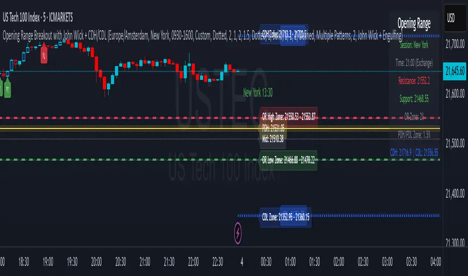
Dskyz (DAFE) Quantum Sentiment Flux - Beginners Dskyz (DAFE) Quantum Sentiment Flux - Beginners:
Welcome to the Dskyz (DAFE) Quantum Sentiment Flux - Beginners , a strategy and concept that’s your ultimate wingman for trading futures like MNQ, NQ, MES, and ES. This gem combines lightning-fast momentum signals, market sentiment smarts, and bulletproof risk management into a system so intuitive, even newbies can trade like pros. With clean DAFE visuals, preset modes for every vibe, and a revamped dashboard that’s basically a market GPS, this strategy makes futures trading feel like a high-octane sci-fi mission.
Built on the Dskyz (DAFE) legacy of Aurora Divergence, the Quantum Sentiment Flux is designed to empower beginners while giving seasoned traders a lean, sentiment-driven edge. It uses fast/slow EMA crossovers for entries, filters trades with VIX, SPX trends, and sector breadth, and keeps your account safe with adaptive stops and cooldowns. Tuned for more action with faster signals and a slick bottom-left dashboard, this updated version is ready to light up your charts and outsmart institutional traps. Let’s dive into why this strat’s a must-have and break down its brilliance.
Why Traders Need This Strategy
Futures markets are a wild ride—fast moves, volatility spikes (like the April 28, 2025 NQ 1k-point drop), and institutional games that can wreck unprepared traders. Beginners often get lost in complex systems or burned by impulsive trades. The Quantum Sentiment Flux is the antidote, offering:
Dead-Simple Setup: Preset modes (Aggressive, Balanced, Conservative) auto-tune signals, risk, and sizing, so you can trade without a quant degree.
Sentiment Superpower: VIX filter, SPX trend, and sector breadth visuals keep you aligned with market health, dodging chop and riding trends.
Ironclad Safety: Tighter ATR-based stops, 2:1 take-profits, and preset cooldowns protect your capital, even in chaotic sessions.
Next-Level Visuals: Green/red entry triangles, vibrant EMAs, a sector breadth background, and a beefed-up dashboard make signals and context pop.
DAFE Swagger: The clean aesthetics, sleek dashboard—ties it to Dskyz’s elite brand, making your charts a work of art.
Traders need this because it’s a plug-and-play system that blends beginner-friendly simplicity with pro-level market awareness. Whether you’re just starting or scalping 5min MNQ, this strat’s your key to trading with confidence and style.
Strategy Components
1. Core Signal Logic (High-Speed Momentum)
The strategy’s engine is a momentum-based system using fast and slow Exponential Moving Averages (EMAs), now tuned for faster, more frequent trades.
How It Works:
Fast/Slow EMAs: Fast EMA (Aggressive: 5, Balanced: 7, Conservative: 9 bars) and slow EMA (12/14/18 bars) track short-term vs. longer-term momentum.
Crossover Signals:
Buy: Fast EMA crosses above slow EMA, and trend_dir = 1 (fast EMA > slow EMA + ATR * strength threshold).
Sell: Fast EMA crosses below slow EMA, and trend_dir = -1 (fast EMA < slow EMA - ATR * strength threshold).
Strength Filter: ma_strength = fast EMA - slow EMA must exceed an ATR-scaled threshold (Aggressive: 0.15, Balanced: 0.18, Conservative: 0.25) for robust signals.
Trend Direction: trend_dir confirms momentum, filtering out weak crossovers in choppy markets.
Evolution:
Faster EMAs (down from 7–10/21–50) catch short-term trends, perfect for active futures markets.
Lower strength thresholds (0.15–0.25 vs. 0.3–0.5) make signals more sensitive, boosting trade frequency without sacrificing quality.
Preset tuning ensures beginners get optimized settings, while pros can tweak via mode selection.
2. Market Sentiment Filters
The strategy leans hard into market sentiment with a VIX filter, SPX trend analysis, and sector breadth visuals, keeping trades aligned with the big picture.
VIX Filter:
Logic: Blocks long entries if VIX > threshold (default: 20, can_long = vix_close < vix_limit). Shorts are always allowed (can_short = true).
Impact: Prevents longs during high-fear markets (e.g., VIX spikes in crashes), while allowing shorts to capitalize on downturns.
SPX Trend Filter:
Logic: Compares S&P 500 (SPX) close to its SMA (Aggressive: 5, Balanced: 8, Conservative: 12 bars). spx_trend = 1 (UP) if close > SMA, -1 (DOWN) if < SMA, 0 (FLAT) if neutral.
Impact: Provides dashboard context, encouraging trades that align with market direction (e.g., longs in UP trend).
Sector Breadth (Visual):
Logic: Tracks 10 sector ETFs (XLK, XLF, XLE, etc.) vs. their SMAs (same lengths as SPX). Each sector scores +1 (bullish), -1 (bearish), or 0 (neutral), summed as breadth (-10 to +10).
Display: Green background if breadth > 4, red if breadth < -4, else neutral. Dashboard shows sector trends (↑/↓/-).
Impact: Faster SMA lengths make breadth more responsive, reflecting sector rotations (e.g., tech surging, energy lagging).
Why It’s Brilliant:
- VIX filter adds pro-level volatility awareness, saving beginners from panic-driven losses.
- SPX and sector breadth give a 360° view of market health, boosting signal confidence (e.g., green BG + buy signal = high-probability trade).
- Shorter SMAs make sentiment visuals react faster, perfect for 5min charts.
3. Risk Management
The risk controls are a fortress, now tighter and more dynamic to support frequent trading while keeping accounts safe.
Preset-Based Risk:
Aggressive: Fast EMAs (5/12), tight stops (1.1x ATR), 1-bar cooldown. High trade frequency, higher risk.
Balanced: EMAs (7/14), 1.2x ATR stops, 1-bar cooldown. Versatile for most traders.
Conservative: EMAs (9/18), 1.3x ATR stops, 2-bar cooldown. Safer, fewer trades.
Impact: Auto-scales risk to match style, making it foolproof for beginners.
Adaptive Stops and Take-Profits:
Logic: Stops = entry ± ATR * atr_mult (1.1–1.3x, down from 1.2–2.0x). Take-profits = entry ± ATR * take_mult (2x stop distance, 2:1 reward/risk). Longs: stop below entry, TP above; shorts: vice versa.
Impact: Tighter stops increase trade turnover while maintaining solid risk/reward, adapting to volatility.
Trade Cooldown:
Logic: Preset-driven (Aggressive/Balanced: 1 bar, Conservative: 2 bars vs. old user-input 2). Ensures bar_index - last_trade_bar >= cooldown.
Impact: Faster cooldowns (especially Aggressive/Balanced) allow more trades, balanced by VIX and strength filters.
Contract Sizing:
Logic: User sets contracts (default: 1, max: 10), no preset cap (unlike old 7/5/3 suggestion).
Impact: Flexible but risks over-leverage; beginners should stick to low contracts.
Built To Be Reliable and Consistent:
- Tighter stops and faster cooldowns make it a high-octane system without blowing up accounts.
- Preset-driven risk removes guesswork, letting newbies trade confidently.
- 2:1 TPs ensure profitable trades outweigh losses, even in volatile sessions like April 27, 2025 ES slippage.
4. Trade Entry and Exit Logic
The entry/exit rules are simple yet razor-sharp, now with VIX filtering and faster signals:
Entry Conditions:
Long Entry: buy_signal (fast EMA crosses above slow EMA, trend_dir = 1), no position (strategy.position_size = 0), cooldown passed (can_trade), and VIX < 20 (can_long). Enters with user-defined contracts.
Short Entry: sell_signal (fast EMA crosses below slow EMA, trend_dir = -1), no position, cooldown passed, can_short (always true).
Logic: Tracks last_entry_bar for visuals, last_trade_bar for cooldowns.
Exit Conditions:
Stop-Loss/Take-Profit: ATR-based stops (1.1–1.3x) and TPs (2x stop distance). Longs exit if price hits stop (below) or TP (above); shorts vice versa.
No Other Exits: Keeps it straightforward, relying on stops/TPs.
5. DAFE Visuals
The visuals are pure DAFE magic, blending clean function with informative metrics utilized by professionals, now enhanced by faster signals and a responsive breadth background:
EMA Plots:
Display: Fast EMA (blue, 2px), slow EMA (orange, 2px), using faster lengths (5–9/12–18).
Purpose: Highlights momentum shifts, with crossovers signaling entries.
Sector Breadth Background:
Display: Green (90% transparent) if breadth > 4, red (90%) if breadth < -4, else neutral.
Purpose: Faster breadth_sma_len (5–12 vs. 10–50) reflects sector shifts in real-time, reinforcing signal strength.
- Visuals are intuitive, turning complex signals into clear buy/sell cues.
- Faster breadth background reacts to market rotations (e.g., tech vs. energy), giving a pro-level edge.
6. Sector Breadth Dashboard
The new bottom-left dashboard is a game-changer, a 3x16 table (black/gray theme) that’s your market command center:
Metrics:
VIX: Current VIX (red if > 20, gray if not).
SPX: Trend as “UP” (green), “DOWN” (red), or “FLAT” (gray).
Trade Longs: “OK” (green) if VIX < 20, “BLOCK” (red) if not.
Sector Breadth: 10 sectors (Tech, Financial, etc.) with trend arrows (↑ green, ↓ red, - gray).
Placeholder Row: Empty for future metrics (e.g., ATR, breadth score).
Purpose: Consolidates regime, volatility, market trend, and sector data, making decisions a breeze.
- VIX and SPX metrics add context, helping beginners avoid bad trades (e.g., no longs if “BLOCK”).
Sector arrows show market health at a glance, like a cheat code for sentiment.
Key Features
Beginner-Ready: Preset modes and clear visuals make futures trading a breeze.
Sentiment-Driven: VIX filter, SPX trend, and sector breadth keep you in sync with the market.
High-Frequency: Faster EMAs, tighter stops, and short cooldowns boost trade volume.
Safe and Smart: Adaptive stops/TPs and cooldowns protect capital while maximizing wins.
Visual Mastery: DAFE’s clean flair, EMAs, dashboard—makes trading fun and clear.
Backtestable: Lean code and fixed qty ensure accurate historical testing.
How to Use
Add to Chart: Load on a 5min MNQ/ES chart in TradingView.
Pick Preset: Aggressive (scalping), Balanced (versatile), or Conservative (safe). Balanced is default.
Set Contracts: Default 1, max 10. Stick low for safety.
Check Dashboard: Bottom-left shows preset, VIX, SPX, and sectors. “OK” + green breadth = strong buy.
Backtest: Run in strategy tester to compare modes.
Live Trade: Connect to Tradovate or similar. Watch for slippage (e.g., April 27, 2025 ES issues).
Replay Test: Try April 28, 2025 NQ drop to see VIX filter and stops in action.
Why It’s Brilliant
The Dskyz (DAFE) Quantum Sentiment Flux - Beginners is a masterpiece of simplicity and power. It takes pro-level tools—momentum, VIX, sector breadth—and wraps them in a system anyone can run. Faster signals and tighter stops make it a trading machine, while the VIX filter and dashboard keep you ahead of market chaos. The DAFE visuals and bottom-left command center turn your chart into a futuristic cockpit, guiding you through every trade. For beginners, it’s a safe entry to futures; for pros, it’s a scalping beast with sentiment smarts. This strat doesn’t just trade—it transforms how you see the market.
Final Notes
This is more than a strategy—it’s your launchpad to mastering futures with Dskyz (DAFE) flair. The Quantum Sentiment Flux blends accessibility, speed, and market savvy to help you outsmart the game. Load it, watch those triangles glow, and let’s make the markets your canvas!
Official Statement from Pine Script Team
(see TradingView help docs and forums):
"This warning may appear when you call functions such as ta.sma inside a request.security in a loop. There is no runtime impact. If you need to loop through a dynamic list of tickers, this cannot be avoided in the present version... Values will still be correct. Ignore this warning in such contexts."
(This publishing will most likely be taken down do to some miscellaneous rule about properly displaying charting symbols, or whatever. Once I've identified what part of the publishing they want to pick on, I'll adjust and repost.)
Use it with discipline. Use it with clarity. Trade smarter.
**I will continue to release incredible strategies and indicators until I turn this into a brand or until someone offers me a contract.
Created by Dskyz, powered by DAFE Trading Systems. Trade fast, trade bold.
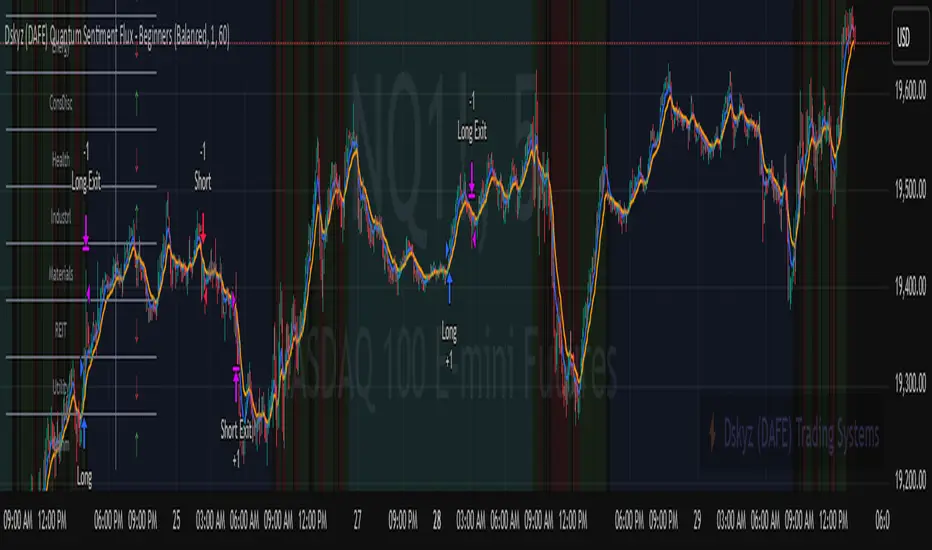
Gradient Sniper Elite🧠 Gradient Sniper Elite — Precision Trend Detection and Tactical Trade Execution for Crypto
Gradient Sniper Elite is a high-performance crypto trend strategy engineered for accuracy, adaptability, and smart execution on the 1-hour timeframe. This script is not just a mashup — it's a purpose-built system that combines trend, momentum, and volume filters in a structured and non-repainting framework designed for optimal entry and exit timing.
🔍 What Makes It Original?
This strategy combines several proven concepts into a unified, precision-calibrated trade engine:
✅ ZLEMA Gradient Filter: A slope-based trend filter that captures the direction and strength of momentum shifts without repainting.
✅ TEMA Confirmation: Triple EMA logic confirms trend acceleration or exhaustion by analyzing layered EMA cross-smoothing.
✅ RMI-Based Trend Direction: Replaces traditional RSI with a Relative Momentum Index (RMI), which smooths price momentum and avoids lag.
✅ ROC & Smoothed CCI: Dual momentum filters ensure that trades align with both velocity and structure of price moves.
✅ Volume Spike Filter: Filters out false breakouts and manipulation by confirming entries only during statistically significant volume surges.
✅ TP1/TP2 Split Take Profit Logic: 50% partial exit at TP1 and full exit at TP2. Ensures flexible profit-taking while maximizing trend continuation gains.
✅ Trend Weakness Exit: Trades are exited cleanly when the trend begins to weaken (as confirmed by RMI flip), preventing overstay and drawdown.
✅ 1-Bar Reversal Delay: The system enforces a 1-bar delay between a trade closure and any potential reversal entry, ensuring clean trend reversals and realistic live trading behavior.
✅ No Stop Loss: This strategy does not use a stop loss. Instead, it exits trades based on trend weakness or TP2 being hit. This avoids premature exits in volatile crypto environments, while maintaining controlled and dynamic trade management logic.
⚙️ How It Works
This strategy uses multi-layered confirmation:
Trend Structure
ZLEMA Gradient: Captures the slope of price action.
White Line + Fast/Slow Tether Lines: Define macro trend structure and act as dynamic S/R filters.
Momentum Alignment
Rate of Change (ROC): Measures directional velocity.
Smoothed CCI: Refines entry timing within the trend.
TEMA: Adds second-layer trend confirmation.
Volume Confirmation
Entry signals are validated by detecting relative volume spikes compared to a moving average baseline, avoiding entries on low-volume or fake breakouts.
Trade Management
Dynamic take-profits (TP1/TP2).
Immediate exit on trend weakening.
No same-bar entry/exit — reversal entries are delayed until after full exit confirmation.
No stop loss — trade management is handled via trend logic and take profit levels.
📊 Dashboard Overview
Gradient Sniper Elite includes a built-in dashboard in the top-right corner of the chart. It dynamically updates on each bar and shows:
📍 Position: Displays "Long", "Short", or "Flat" depending on the active trade
💰 Entry Price: The exact price where the trade was entered
📈 Unrealized %: Current profit/loss as a percentage
💵 Unrealized $: Estimated PnL in dollars, scaled to your backtest capital
📊 Trades / Win Rate: Live counter for total trades, win/loss count, and win rate
🎯 TP1 Hit / TP2 Hit: Shows ✅ or ❌ depending on whether each target level was reached during the current trade
This dashboard helps you monitor trade status, track live performance, and validate signal behavior in real time — all without repainting or relying on external tools.
📈 How to Use
Timeframe: Optimized for the 1-hour timeframe, but adaptable.
Asset Class: Primarily built for crypto markets, especially fast-moving alts like AVAX, LINK, QNT, etc.
Trade Mode: Supports long and short trades with clean reversal logic.
Dashboard: Live stats including position status, TP1/TP2 hit, win rate, and real-time PnL tracking.
Backtest Ready: Built with full compliance to TradingView backtest engine — results are realistic and match live-bar behavior.
⚠️ No Repainting — No Guesswork
Every element in this script is designed to work with confirmed bar data only. There is zero forward-looking logic. This makes Gradient Sniper Elite fully compatible with both backtesting and live algo execution.
🧩 Why This Isn’t Just a Mashup
Each indicator in this strategy has a specific role:
ZLEMA: Core trend slope engine.
TEMA: Trend reinforcement.
RMI: Directional decision layer.
CCI & ROC: Entry timing refinement.
Volume Filter: Risk filtering.
They’re not merged randomly, but combined in sequence to eliminate noise and optimize entries.
📌 Disclaimer
This script is for informational and educational purposes only. It does not constitute financial advice or a recommendation to buy or sell any asset. Always do your own research and use appropriate risk management when trading. Past performance does not guarantee future results.
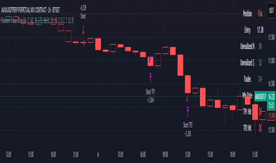
Adaptive RSI with Real-Time Divergence [AIBitcoinTrend]👽 Adaptive RSI Trailing Stop (AIBitcoinTrend)
The Adaptive RSI Trailing Stop is an indicator that integrates Gaussian-weighted RSI calculations with real-time divergence detection and a dynamic ATR-based trailing stop. This advanced approach allows traders to monitor momentum shifts, identify divergences early, and manage risk with adaptive trailing stop levels that adjust to price action.
👽 What Makes the Adaptive RSI with Signals and Trailing Stop Unique?
Unlike traditional RSI indicators, this version applies a Gaussian-weighted smoothing algorithm, making it more responsive to price action while reducing noise. Additionally, the trailing stop feature dynamically adjusts based on volatility and trend conditions, allowing traders to:
Detects real-time divergences (bullish/bearish) with a smart pivot-based system.
Filter noise with Gaussian weighting, ensuring smoother RSI transitions.
Utilize crossover-based trailing stop activation, for systematic trade management.
👽 The Math Behind the Indicator
👾 Gaussian Weighted RSI Calculation
Traditional RSI calculations rely on simple averages of gains and losses. Instead, this indicator weights recent price changes using a Gaussian distribution, prioritizing more relevant data points while maintaining smooth transitions.
Key Features:
Exponential decay ensures recent price changes are weighted more heavily.
Reduces short-term noise while maintaining responsiveness.
👾 Real-Time Divergence Detection
The indicator detects bullish and bearish divergences using pivot points on RSI compared to price action.
👾 Dynamic ATR-Based Trailing Stop
Bullish Trailing Stop: Activates when RSI crosses above 20 and dynamically adjusts based on low - ATR multiplier.
Bearish Trailing Stop: Activates when RSI crosses below 80 and adjusts based on high + ATR multiplier
This allows traders to:
Lock in profits systematically by adjusting stop-losses dynamically.
Stay in trades longer while maintaining adaptive risk management.
👽 How It Adapts to Market Movements
✔️ Gaussian Filtering ensures smooth RSI transitions while preventing excessive lag.
✔️ Real-Time Divergence Alerts provide early trade signals based on price-RSI discrepancies.
✔️ ATR Trailing Stop dynamically expands or contracts based on market volatility.
✔️ Crossover-Based Activation enables the stop-loss system only when RSI confirms a momentum shift.
👽 How Traders Can Use This Indicator
👾 Divergence Trading
Traders can use real-time divergence detection to anticipate reversals before they happen.
Bullish Divergence Setup:
Look for RSI making a higher low, while price makes a lower low.
Enter long when RSI confirms upward momentum.
Bearish Divergence Setup:
Look for RSI making a lower high, while price makes a higher high.
Enter short when RSI confirms downward momentum.
👾 Trailing Stop Signals
Bullish Signal and Trailing Stop Activation:
When RSI crosses above 20, a trailing stop is placed using low - ATR multiplier.
If price crosses below the stop, it exits the trade and removes the stop.
Bearish Signal and Trailing Stop Activation:
When RSI crosses below 80, a trailing stop is placed using high + ATR multiplier.
If price crosses above the stop, it exits the trade and removes the stop.
This makes trend-following strategies more efficient, while ensuring proper risk management.
👽 Why It’s Useful for Traders
✔️ Dynamic and Adaptive: Adjusts to changing market conditions automatically.
✔️ Noise Reduction: Gaussian-weighted RSI reduces short-term price distortions.
✔️ Comprehensive Strategy Tool: Combines momentum detection, divergence analysis, and automated risk management into a single indicator.
✔️ Works Across Markets & Timeframes: Suitable for stocks, forex, crypto, and futures trading.
👽 Indicator Settings
RSI Length: Defines the lookback period for RSI smoothing.
Gaussian Sigma: Controls how much weight is given to recent data points.
Enable Signal Line: Option to display an RSI-based moving average.
Divergence Lookback: Configures how far back pivot points are detected.
Crossover/crossunder values for signals: Set the crossover/crossunder values that triggers signals.
ATR Multiplier: Adjusts trailing stop sensitivity to market volatility.
Disclaimer: This indicator is designed for educational purposes and does not constitute financial advice. Please consult a qualified financial advisor before making investment decisions.
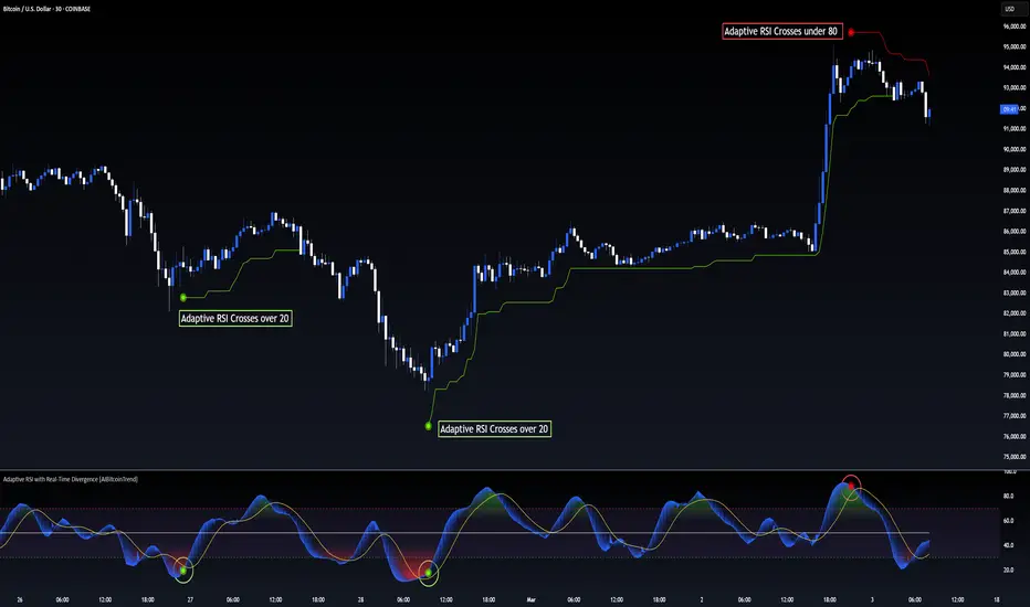
Btc and Eth 5 min winnerWhat the Strategy Does
Finding the Trend (Like Watching the Bus Move): The strategy uses special tools called Hull Moving Averages (HMAs) to figure out if Bitcoin (BTC) Ethereum (ETH) prices are generally going up or down. It looks at short-term (5 minutes) and long-term (10 minutes) price movements to make sure the “bus” (the market) is moving strongly in one direction—up for buying, down for selling.
Spotting Good Times to Jump On (Buy or Sell Signals): It looks for two types of opportunities:
Pullbacks: When the price dips a little while still moving up (like the bus slowing down but not stopping), it’s a chance to buy.
Breakouts: When the price suddenly jumps higher after being stuck (like the bus speeding up), it’s another chance to buy. It does the opposite for selling when prices are dropping.
It also checks if there’s enough “passenger activity” (volume) and momentum (speed of price change) to make sure it’s a good move.
Avoiding Traffic Jams (Filters): The strategy uses tools like RSI (to check if the market’s too fast or too slow), volume (to see if enough people are trading), and ATR (to measure how wild the price swings are). It skips trades if things look too chaotic or if the trend isn’t strong enough.
Setting Safety Stops and Profit Targets: Once you’re on the “bus,” it sets rules to protect you:
Stop-Loss: If the price moves against you by a small amount (0.5% of the typical price swing), you jump off to avoid losing too much—think of it as getting off before the bus crashes.
Take-Profit: If the price moves in your favor by a small amount (1.0% of the typical swing), you cash out—imagine getting off at your stop with a profit.
Trailing Stop: If the price keeps moving your way, it adjusts your exit point to lock in more profit, like moving your stop closer as the bus keeps going.
Using Leverage (10x Boost): This strategy uses 10x leverage on Binance futures, meaning for every $1 you have, you trade like you have $10. This can make profits (or losses) 10 times bigger, so it’s risky but can be rewarding if you’re careful.
Why 5 Minutes and Bitcoin and Ethereum?
5-Minute Chart: This is like checking the bus every 5 minutes to make quick, small trades—perfect for fast, short profits.
Bitcoin Ethereum (BTC/USD)(ETH/USD): It’s the most popular and liquid crypto, so there’s lots of activity, making it easier to jump on and off without getting stuck.
Why It Aims for 90% Wins (But Be Realistic)
The goal is to win 9 out of 10 trades by being super picky about when to trade—only jumping on when the trend, momentum, and volume are all perfect. But in real trading, markets can be unpredictable, so 90% is very hard to achieve. Still, this strategy tries to be as accurate as possible by avoiding bad moves and focusing on strong trends.
Risks for a New Trader
Leverage: Trading with 10x leverage means small price moves can lead to big losses if you’re not careful. Start with a demo account (pretend money) on TradingView or Binance to practice.
Learning Curve: This strategy uses technical terms (like HMAs, RSI) and tools you’ll need to learn over time. Don’t rush—just practice and ask questions!
How to Use It
Go to TradingView, load this strategy on a 5-minute BTC/USD futures chart on Binance.
Watch the green triangles (buy signals) and red triangles (sell signals) on the chart—they tell you when to trade.
Use the stops and targets to manage your trades—don’t guess, let the strategy guide you.
Start small, learn from each trade, and don’t risk money you can’t afford to lose.
This is like learning to ride a bike—start slow, practice, and you’ll get better. If you have more questions or want simpler tips, feel free to ask! Trading can be fun and rewarding, but it takes patience and practice.

ATR Trailing Stop by GideonMATR Trailing Stop Indicator
This ATR Trailing Stop Indicator is designed for traders who wish to enhance their exit strategies by leveraging volatility-based stops. It offers a systematic approach to trend management and risk control, enabling traders to capture extended trends while protecting their capital during market reversals. Works on Indian Indices as well.
Overview:
The ATR Trailing Stop indicator is a dynamic trend-following tool that adjusts stop levels based on market volatility. By incorporating the Average True Range (ATR), the indicator provides a flexible exit strategy that adapts to changing market conditions, helping traders lock in profits during trends and limit losses during reversals.
How It Works:
True Range and ATR Calculation:
The indicator first calculates the True Range (TR) for each bar, defined as the maximum of:
The difference between the high and low,
The absolute difference between the high and the previous close, and
The absolute difference between the low and the previous close.
Using the TR values, the ATR is computed over a user-defined period (default is 14 bars) with an option to use either a Simple Moving Average (SMA) or an Exponential Moving Average (EMA) as the smoothing method.
Trailing Stop Determination:
Two potential stop levels are calculated:
For an uptrend, the stop is determined as:
Stop = Close – (Multiplier × ATR)
For a downtrend, the stop is:
Stop = Close + (Multiplier × ATR)
The indicator maintains a persistent trailing stop that dynamically adjusts:
In an uptrend, the trailing stop only moves upward (or remains flat) to secure gains.
In a downtrend, it only moves downward, thereby protecting the position from excessive losses.
A reversal in trend is identified when the price crosses the trailing stop level, at which point the indicator flips the trend and resets the stop level accordingly.
Rationale:
Utilizing the ATR for trailing stops ensures that the stop levels are directly influenced by market volatility. This dynamic adjustment helps accommodate the natural price fluctuations of the market, providing a more adaptive risk management tool compared to fixed stop-loss levels. The approach is particularly useful in volatile markets where traditional static stops might be triggered prematurely.
Customization:
Key parameters that can be adjusted include:
ATR Period: The number of bars used to calculate the ATR.
ATR Multiplier: The factor that determines how far the trailing stop is set from the current price.
Smoothing Method: Option to choose between SMA and EMA for ATR calculation, allowing traders to tailor the sensitivity of the indicator to their specific trading style.

Altcoins DCA ScalperIntroduction
The Altcoins DCA Scalper is a Pine Strategy Script designed to automate Altcoins trading through 3Commas integration. It implements a Dollar-Cost Averaging (DCA) strategy that expands upon 3Commas' standard DCA capabilities, helping to manage risk while trading both long and short positions automatically.
This tool aims to assist both beginners exploring automated trading and experienced 3Commas users seeking dynamic DCA automation. The script is specifically designed for the 1-minute timeframe , where it has shown a good balance between performance and risk management. Complete setup typically takes less than 10 minutes, with a detailed guide making configuration straightforward for users of all experience levels.
------------------------------
🔶 What is DCA?
------------------------------
Dollar-cost averaging (DCA) refers to the practice of gradually increasing your position size at lower prices when trading long, or at higher prices when trading short, to achieve a better average entry price if the market moves against the initial entry . Instead of investing all capital at once, which could result in a significant drawdown if the price moves unfavorably, DCA spreads entries across different price levels to help manage potential drawdowns as they occur.
In this script, DCA is implemented through a system that:
🔹 Triggers safety orders only when/if needed (if take profit isn't reached quickly)
🔹 Dynamically adjusts order sizing based on market volatility
🔹 Automatically reduces take profit targets after each DCA order to increase the likelihood of a positive outcome
🔹 Can handle drawdowns depending on market volatility and settings
The images below illustrate two scenarios: one where an entry reaches the take profit directly, without activating DCA orders, and another where DCA is utilized, with the order closing positively after two DCA orders.
Case 1: Order closes in profit after entry
Case 2: Order closes in profit after 2 DCA orders (dynamically placed based on trend and volatility)
This DCA implementation aims to enhance standard 3Commas DCA by adding market-adaptive features while maintaining risk management principles.
------------------------------
🔶 Could this strategy script benefit you?
------------------------------
This script may be helpful if you are:
✅ Looking to automate your trading through 3Commas integration while maintaining full control of your assets
✅ Wanting to enhance 3Commas' standard DCA with market-adaptive features that consider:
Multi-timeframe trend analysis
Real-time volatility assessment
Dynamic safety order sizing and timing
✅ Seeking to minimize chart monitoring through full automation of:
Entry and exit decisions
Safety order management
Risk controls
✅ Interested in comprehensive performance tracking with:
Real-time position metrics
Detailed backtesting capabilities
Risk/reward analysis
Backtesting Metrics (script performance over the backtesting period - which is approx. 15 days on the 1min timeframe with the TradingView Pro Plan):
Current/Open Deal Metrics (the deal is currently under DCA, and waiting for further actions to close):
✅ Looking for trading automation that remains easy to set up and use
Note: While this script provides trading automation, successful trading requires proper education, risk management, and regular performance monitoring. No automated tool can guarantee trading success or profits.
------------------------------
🔶 How it Works
------------------------------
The Altcoins DCA Scalper provides trading automation through:
Market Analysis
* Multi-timeframe trend analysis (1m to 1d) for market direction and entry validation
* Volatility assessment (1h, 4h, 24h) benchmarked against TOTAL3 (excluding Top10 Altcoins and Stablecoins)
* Real-time adjustment of DCA parameters based on:
* Current volatility class (low/medium/high) vs. overall Altcoins market
* Market trend strength
* Price action dynamics
Trading Execution
* Position opening aligned with detected market trends
* "Beast Mode" base order sizing that increases position size during strong trends
* Dynamic take-profit targets that automatically reduce after each safety order to increase the likelihood of positive exits
* Dynamic DCA with safety orders that can:
* Adapt timing based on volatility
* Scale order sizes based on market conditions
* Handle 30-50% drawdowns depending on volatility class
* Execute up to 6 safety orders per position
Risk Management
* Emergency exits during extreme market events:
* "Black Swan" protection for long positions
* "God-Candle" protection for short positions
* Configurable stop-loss with volatility-based placement
* Trend-switch management with automated position reversal
* Position aging controls to prevent capital lock-up
* Leveraged trading protection with a pre-liquidation exit system
Integration & Automation
* Quick setup with two 3Commas bots (typically under 10 minutes)
* Fully automated signal generation and execution through 3Commas
* Detailed performance tracking including:
* Real-time position metrics
* DCA depth analysis
* Win rate and ROE calculations
* Pre-configured settings optimized for most pairs
* Multiple customization options for experienced users
Note: While this strategy employs automation and risk management, trading always carries the risk of loss. No system can guarantee profits, and market conditions significantly impact performance. Always do your own research and monitor your positions closely.
------------------------------
How to Use
------------------------------
Setting up the Altcoins DCA Scalper is quick and facilitated by the User Interface:
1️⃣ 3Commas/TradingView Setup
* Create two 3Commas accounts if using the FREE plan:
* One account for Long Bot
* One account for Short Bot
* This split allows full functionality while staying within 3Commas' free tier limits
* You do not need two separate accounts if you have a Paid 3Commas subscription
* While a free TradingView account works with the script, it limits you to one trading pair and a 4-day backtesting history. A paid TradingView subscription removes these limitations (such as the "Essential" plan).
2️⃣ Bot Configuration
* Create one Long and one Short DCA Bot in 3Commas
* Follow the setup guide available in the script itself for hassle-free configuration
* Copy Bot IDs and Email Token for script connection
* No complex settings needed - the script manages all DCA parameters by itself
3️⃣ Script Implementation
* Apply the script to your TradingView charts
* Use the built-in backtesting to analyze performance on different pairs
* Focus on USDT.P futures pairs with good volatility
4️⃣ Trading Activation
* Create TradingView alerts for each trading pair you want to activate
* Example: Set an alert for BINANCE: XRPUSDT.P following the in-script guide
* The script automatically manages all aspects:
* Entry and exit decisions
* DCA execution
* Risk management
* Position monitoring
Capital Requirements
* Important: Ensure sufficient capital to cover all activated pairs
* Consider volatility class when allocating capital to specific pairs
Once setup is complete, the script operates fully automatically while you maintain complete control of your funds through 3Commas and your exchange.
Note: While the setup is straightforward, always start with a small number of pairs and monitor performance before expanding. Trade responsibly and never risk more than you can afford to lose.
------------------------------
Explaining the Settings
------------------------------
The Altcoins DCA Scalper offers mulitple customization options during the setup process. All settings include detailed tooltips and default values.
Core Settings Sections:
1️⃣ 3Commas Connection
* Bot IDs and Email Token configuration
* Leverage settings (1x to 5x supported)
* Detailed 3Commas bot setup guide included
* Automatic bot control configuration
2️⃣ Trading Parameters
* Capital allocation per trade
* Timeframe verification
* Alert system setup
* Backtesting period control
* Performance tracking preferences
3️⃣ Advanced Features
🔹 Risk Management Suite
* Emergency exit controls (to strengthen protection against extraordinary market events)
* Customizable stop-loss system
* Trend-based exit management
* Position aging controls
* Liquidation protection features
* Advanced DCA controls
🔹 Performance Analytics
* Real-time position monitoring
* Comprehensive backtesting metrics
* DCA depth analysis
* Win rate calculations
* Capital efficiency tracking
🔹 Technical Optimizations
* Exchange minimum order adjustment
* Trading pair name override capability
* System stability controls
* Error handling mechanisms
🔹 Interface Customization
* Theme selection
* Chart overlay options
* Warning display preferences
* Performance metrics visibility
All settings come pre-configured but can be fully customized based on your trading preferences and risk tolerance. The script includes tooltips and setup guides for each option.
Note: While default settings may be tested, market conditions vary and all trading involves risk. Monitor performance and adjust settings according to your risk management requirements.
------------------------------
Frequently Asked Questions
------------------------------
Here are some common questions you may have, and our answers:
❓ Is this tool only for experts? I'm new to algo trading, can I use it?
No, the Altcoins DCA Scalper could be used by both beginners and experienced traders. The setup process is guided, and the algorithm handles all the calculations in the background.
❓ I'm not familiar with 3Commas. Is that a problem?
While the script is designed to work with 3Commas, a step-by-step guide is provided within the script to help you set up your 3Commas accounts and bots, if needed.
❓ Do I need to constantly monitor the script after it's set up?
No, after the initial setup and configuration, the script operates autonomously. It handles all aspects of trading including entries, exits, DCA management, and risk controls. However, we recommend:
* Checking performance metrics daily
* Reviewing position statistics weekly
* Adjusting pair selection monthly based on performance
* Monitoring overall market conditions that might require adjustments
❓ Can I use it with leverage?
Yes, the script is designed to work with leverage up to 5x on perpetual futures pairs (USDT.P). It includes specific features for leveraged trading:
* Dynamic safety order placement based on distance to liquidation
* Pre-liquidation exit system to minimize exchange fees
* Adjustable take-profit targets optimized for leveraged positions
* Emergency exit system for extreme market movements
* Optional risk controls specific to leverage:
* Automatic exit in the liquidation danger zone
* Position size scaling based on leverage level
* Safety order adjustments for different leverage settings
While leverage can amplify returns, it also increases risk. We recommend starting with lower leverage (2x), or no leverage at all, until familiar with the script's operation.
❓ Does this script guarantee profits?
No, no script or trading strategy can guarantee profits. The Altcoins DCA Scalper provides a framework for implementing an automated DCA strategy, but your success will depend on many different factors and conditions.
❓ Do I need to understand the complex algorithms used in the script?
No, it’s not necessary. The logic is handled by the script, and you do not need to understand every detail to use it effectively. However, a basic knowledge of DCA concepts will be beneficial.
❓ Can I use this script with spot or leveraged trades?
The script is optimized for USDT.P pairs (perpetual futures) with leverage up to 5x. This allows:
* Automatic long/short position management
* Increased capital utilization
* Full DCA functionality without holding the underlying assets
* Enhanced risk management features specific to futures
While spot trading is possible, it requires holding underlying assets for shorts and doesn't access the script's full capabilities.
❓What timeframe should I use?
This script is optimized for the 1-minute timeframe , which is the recommended setting for the best balance between performance, capital efficiency, and risk. While we recommend using the tool on the 1 minute TF, it would work on other timeframes too.
❓ What happens if my internet/computer goes down?
Since the script sends signals from Tradingview to 3Commas (which executes trades on your exchange), your positions and DCA management continue to function even if your TradingView chart is closed or your computer is off. The script only needs to be active to generate new signals.
❓ How are the DCA parameters determined?
The script dynamically adjusts DCA parameters based on:
* The pair's volatility class (compared to the overall altcoin market)
* Current market conditions and volatility
* Position direction (long/short)
* Leverage settings
* Number of safety orders already executed
This allows for adaptive/dynamic DCA compared to static or %-based parameters.
❓ What exchanges are supported?
The script works with any exchange supported by 3Commas for futures trading (approximately 15 different crypto Exchanges). However, it's optimized for Binance Futures (USDT.P pairs) due to its high liquidity and for consistency.
❓ What happens during extreme market conditions?
The script includes some (optional) protective measures that can be activated:
* Emergency exits during sharp and abnormal market moves
* Automatic adjustment of DCA parameters during high volatility
* Position closure on significant trend changes
* Special handling of aged positions
These features aim to protect capital during unusual market conditions.
❓How many pairs can I trade simultaneously?
This depends on your total capital. As a general indication, define the number of pairs to activate based on:
* Total available capital
* Desired position size per pair
* Risk tolerance
* Pairs' volatility class
------------------------------
Final Thoughts
------------------------------
We believe that your trading performance will greatly depend on your selection of appropriate trading pairs for this script (high volatility), and your commitment to regularly monitoring its performance and adjust the settings, rather than on the script alone.
------------------------------
⚠️ Risk Disclaimer
------------------------------
Remember that trading involves risk, and most day traders experience losses. This script is for educational and informational purposes only. Past performance does not guarantee future results. This is not financial advice, and you should always do your own research (DYOR). Trade responsibly with capital you can afford to lose.
The Altcoins DCA Scalper is an independent tool and is not endorsed, connected, or validated by TradingView.
3Commas is a third-party service, and TradingView is not responsible for the 3Commas integration or the performance of 3Commas bots. You are solely responsible for the security and management of your 3Commas account. Do not share your 3Commas access credentials (like login information, Bots-ID, Email Token) with anyone. The Author of the script has no access to such information, and nobody (but you) should.

Intraday Golden duckKey Components
Plotting DTR Levels
DTR High 1 & Low 1 are plotted with a bold green and red line (Major Levels).
DTR High 2 & Low 2 are plotted with a lighter green and red line (Minor Levels).
This visualizes potential breakout and stop-loss zones.
Defining Market Hours
The strategy runs only between:
Start Time: 9:15 AM (Market Open)
End Time: 3:00 PM (Market Close)
Trades can only occur during this period.
Avoiding Multiple Trades Per Day
A boolean variable trade_taken_today ensures that:
Only one trade is executed per day (either Buy or Sell).
It resets at the beginning of a new trading day.
Entry Conditions
A long position (Buy) is entered when:
The market is open.
The close price breaks above dtr_high_1.
No other trade has been executed yet.
A short position (Sell) is entered when:
The market is open.
The close price drops below dtr_low_1.
No other trade has been executed yet.
Stop-Loss Conditions
To protect against large losses, stop-loss levels are placed at DTR 2 levels:
For Long Trades: If price falls below dtr_high_2, the trade exits.
For Short Trades: If price rises above dtr_low_2, the trade exits.
Using Parabolic SAR for Additional Exit Signals
The Parabolic SAR (PSAR) is used to trail stop-loss:
Long Exit: If price falls below PSAR, the position is closed.
Short Exit: If price rises above PSAR, the position is closed.
Universal Exit Condition (3:00 PM)
At exactly 3:00 PM, all positions are forcefully closed, ensuring no overnight risk.
Execution Logic
If Buy Condition is met → Enter Long position.
If Sell Condition is met → Enter Short position.
If Stop-Loss or PSAR condition triggers → Exit the trade.
At 3:00 PM, close all positions.
Key Features & Benefits
✅ Intraday Only: No overnight risk.
✅ One Trade per Day: Avoids overtrading.
✅ Dynamic Levels: Adapts to market volatility.
✅ PSAR Protection: Helps reduce drawdowns.
✅ Universal Exit: Ensures systematic closing.
This strategy is designed for traders looking for a systematic, rule-based approach to intraday trading using price action and volatility expansion principles. 🚀
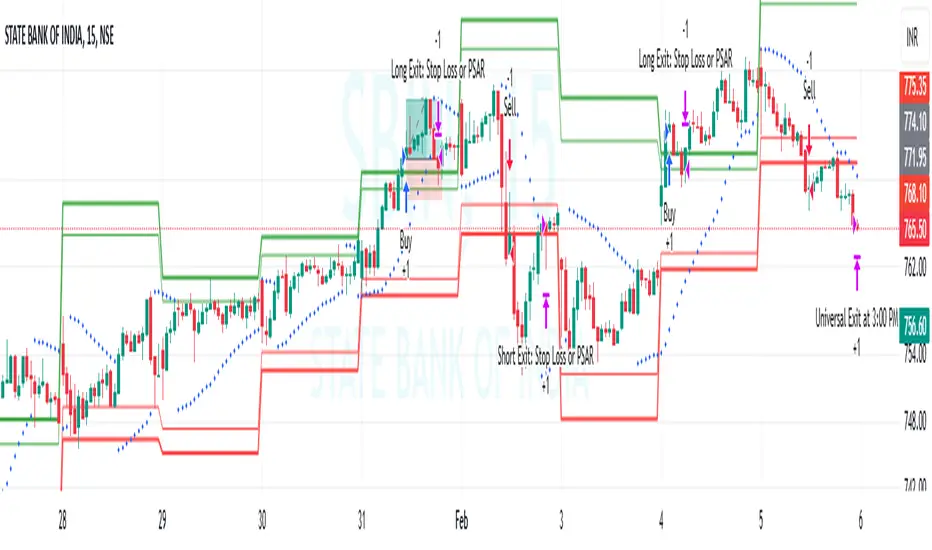
Fibonacci Extension Strt StrategyCore Logic and Steps:
Weekly Trend Identification:
Find the last significant Higher High (HH) and Lower Low (LL) or vice-versa on the Weekly timeframe.
Determine if it's an uptrend (HH followed by LL) or a downtrend (LL followed by HH).
Plot a Fibonacci Extension (or Retracement in reverse order) from the swing point determined to the other significant swing point.
Weekly Retracement Levels:
Display horizontal lines at the 0.236, 0.382, and 0.5 Fibonacci levels from the weekly extension.
Monitor price action on these levels.
Daily Confirmation:
When price hits the Fib levels, examine the Daily chart.
Look for a rejection wick (indicating the pull back is ending) on the identified weekly retracement levels.
Confirm that the price is indeed starting to continue in the direction of the original weekly trend.
Four-Hour Entry:
On the 4H timeframe, plot a new Fib Extension in the opposite direction of the weekly.
If it's an uptrend, the Fib is plotted from last swing low to its swing high. If the weekly trend was bearish the Fib will be plotted from last swing high to the swing low.
Generate an entry when price breaks the high of that candle.
Trade Management:
Entry is on the breakout of the current candle.
Stop Loss: Place the stop loss below the wick of the breakout candle.
Take Profit 1: Close 50% of the position at the 0.5 Fibonacci level. Move the stop loss to breakeven on this position.
Take Profit 2: Close another 25% of the position at the 0.236 Fib level.
Trailing Take Profit: Keep the last 25% open, using a trailing stop loss. (You'll need to define the logic for the trailing stop, e.g., trailing stop using the last high/low)
How to Use in TradingView:
Open a TradingView Chart.
Click on "Pine Editor" at the bottom.
Copy and paste the corrected Pine Script code.
Click "Add to Chart".
The indicator should now be displayed on your chart.