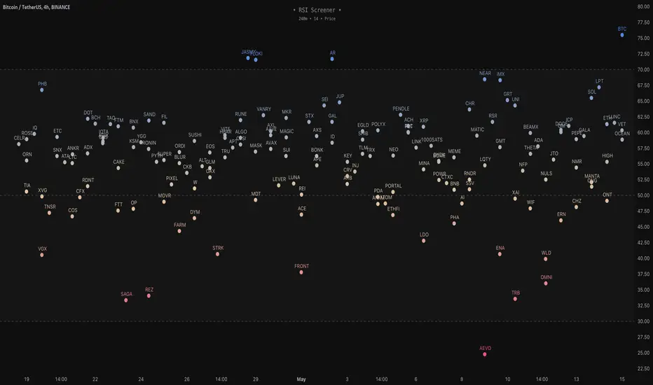
RSI Screener / Heatmap - By LeviathanThis script allows you to quickly scan the market by displaying the RSI values of up to 280 tickers at once and visualizing them in an easy-to-understand format using labels with heatmap coloring.
📊 Source
The script can display the RSI from a custom timeframe (MTF) and custom length for the following data:
- Price
- OBV (On Balance Volume)
- Open Interest (for crypto tickers)
📋 Ticker Selection
This script uses a different approach for selecting tickers. Instead of inputting them one by one via input.symbol(), you can now copy-paste or edit a list of tickers in the text area window. This approach allows users to easily exchange ticker lists between each other and, for example, create multiple lists of tickers by sector, market cap, etc., and easily input them into the script. Full credit to @allanster for his functions for extracting tickers from the text. Users can switch between 7 groups of 40 tickers each, totaling 280 tickers.
🖥️ Display Types
- Screener with Labels: Each ticker has its own color-coded label located at its RSI value.
- Group Average RSI: A standard RSI plot that displays the average RSI of all tickers in the group.
- RSI Heatmap (coming soon): Color-coded rows displaying current and historical values of tickers.
- RSI Divergence Heatmap (coming soon): Color-coded rows displaying current and historical regular/hidden bullish/bearish divergences for tickers.
🎨 Appearance
Appearance is fully customizable via user inputs, allowing you to change heatmap/gradient colors, zone coloring, and more.
在脚本中搜索"text"
KeitoFX Dynamic Indicator Free vers.This script represents a versatile dynamic indicator called "KeitoFX Dynamic Indicator Free version." It is developed by the author "KeitoFX" and operates as a custom indicator overlaying on financial charts. The indicator utilizes a unique algorithm to dynamically identify bullish and bearish candlestick patterns with specific criteria.
Key Features:
- The indicator visually marks bullish and bearish candlestick patterns using triangle shapes, providing quick visual cues to traders.
- Bullish patterns are detected when the closing price is higher than the opening price and the high and low prices of the candlestick form a narrow range.
- Bearish patterns are identified when the closing price is lower than the opening price, and the high and low prices also form a narrow range.
The indicator incorporates flexible settings that users can customize to fit their trading preferences:
- Users can choose the table's placement, either at the "Top Right," "Middle Right," or "Bottom Right" of the chart.
- Customizable dimensions for the width and height of the table are available.
- Adjustable text size settings ranging from "Auto" to "Huge" are provided for the displayed text.
- A descriptive table containing trading rules and conditions is optionally displayed below the price chart.
Additional Information:
- The indicator's color scheme is harmonious, with shades of purple and neutral tones.
- The "Require FVG" setting influences the pattern detection's sensitivity.
- A dynamic standard deviation is calculated based on the selected displacement settings and historical candle ranges.
- A "FVG" condition enhances pattern accuracy.
- Bullish and bearish pattern detection includes overlapping with other predefined arrays to increase pattern significance.
Note:
This indicator is provided under the Mozilla Public License 2.0, as indicated by the source code comment at the beginning of the script. Users are encouraged to review and comply with the license terms when using this indicator in their trading activities.

Any Screener (Multiple)I suppose it's time to publish something relatively useful :). Here's the first try, Any Screener.
This script is an advanced version of the Alphatrend - Screener that I've coded as a humble "thank you" to Kıvanç Özbilgiç (KivancOzbilgic), who always inspired me.
INTRODUCTION
I developed this version with a unique method because I couldn't find an example with the following features:
It presents the valid signal status of multiple indicators for 15 different symbols in the form of a report.
It indicates how many bars have passed after the signal has occurred.
It indicates the signal direction with dynamic colors and chars.
It can also be used for data (just indicator value) that is only intended to be displayed as text. (Default color is grey).
Long and short signals can optionally be ploted on the chart.
It includes advanced configuration settings.
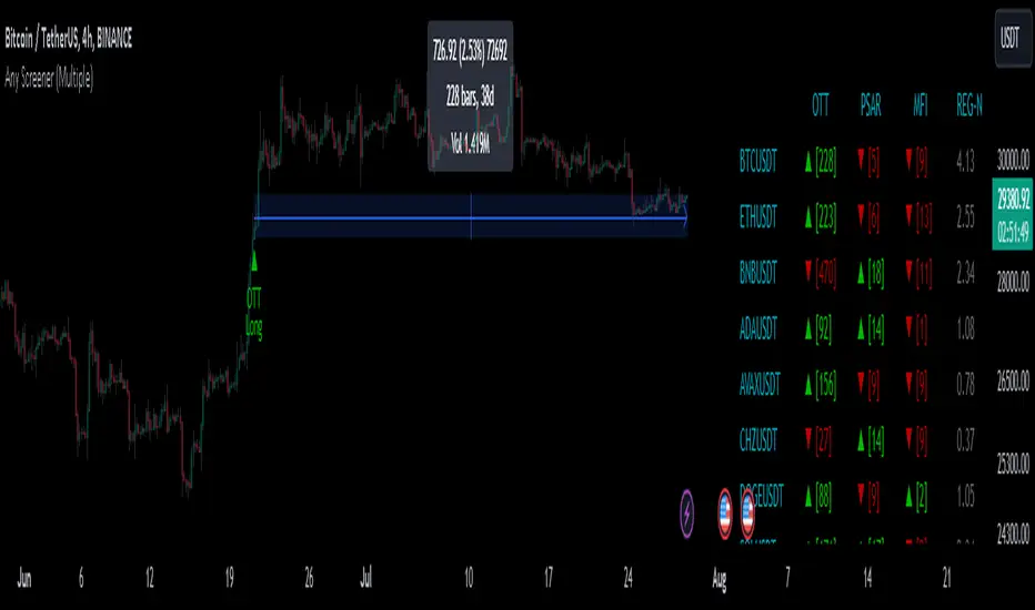
USAGE OF PANEL
The screener panel is simple to use. On the far left, assets are listed. The names of the indicators appear at the top. In the column with the name of each indicator, the signals of that indicator appear as green or red. The green ones represent the long signals (uptrend) and the red ones represent the short signals (down trend). The numbers in square brackets indicate how many bars have passed after the last signal has occurred. (For example: According to the indicator at the top, when the green bullish triangle and 21 appeared on allign of BTCUSDT, Bitcoin switched to buy signal 21 bars ago. A tip : If the signal distance is 0, the signal occurred at the current bar. It is recommended to wait for the bar to close before entering the trade). Signal distance is an essential output for both manual and algorithmic trading. Users often require mentioned data the most during real time trading.
THE SCRIPT
There are two sections in the script; indicators and screener.
SECTION 1 : "INDICATORS"
In the indicator section, you'll find efficient details about switch methods, normalization, avoid pyramyding (in momentum oscillators) etc. On the other hand, I intended to present a "how to example" of a multiple screener, so it has to include more than one indicator.
OTT : Optimized Trend Tracker is developed by dear Anıl Özekşi, known as the "Old Fisherman" :). In my opinion, it is a pretty cool trend-following indicator that offers a mathematical elegance. This indicator aim to detect the current market trend direction, the indicator detect an up-trending market when the support line is superior to the OTT, and a down trending market when the support line is inferior to the OTT. It has three parameters; moving average type, length and percentage. In this version when the percentage parameter is set to 0.0, OTT turns into the selected moving average. And the signals are generated by the crossing of the closing price. It means, this screener is able to compile and present status of moving averages as well. Also VAR (VIDYA) and EVWMA has been re-designed, both moving averages no longer start at zero at the beginning of the chart (That was a big problem for backtests).
PSAR : J. Welles Wilder's Parabolic Stop And Reversal is an important trend following indicator. PSAR detects an up-trending market when below the market price and a down-trend when above. It can work in harmony with OTT according to the parameter combinations.
OSCILLATORS : Also optional three momentum oscillators have been added. MFI (Money Flow Index), RSI (Relative Strength Index) and STOCH (Stochastic %k). All three oscillators are widely used in markets and quite successful in explaining price movements by using different sources. Oscillators generate long and short signals based on oversold and overbought parameters.
VOLATILITY & TREND : There are three optional indicators. ADX (Average Directional Index), BBW-N (Normalized Bollinger Bandwidth) and REG-N (Normalized value of standard error of linear regression). These three indicators don't generate any long or short signals. Instead, they are used to measure the strength of trends and volatility. Therefore, only the numerical results (0-100) are displayed in screener panel and it is grey. (Note : The second length parameter of ADX has the same value with the first one. Bollinger Bandwith's multiplier is 2.0. REG-N is a variable that developed by Paul Kirshenbaum for Kirshenbaum Bands.)
SECTION 2 : "SCREENER"
The second section processes the main idea. This Screener model is based on generating an integer direction variable from boolean signals. The direction value serves multiple purposes: calculating the distance of signal, determining the color based on the direction, and creating "clean" data for the security function. The final step is to present the obtained data as text to the user.
HOW CAN I "SCREEN" MY CONDITIONS?
That's piece a cake, delete the Section 1 in the script :). If you change totally 11 variables according to your own strategy, you can create your new screener! The method is explained at lines 169-171.
SINCERELY THANKS
To allanster for patiently answering my primitive questions,
And to KivancOzbilgic for mind blowing suggestions (especially while we're drinking Raki) :)...
DISCLEIMER
This is just an indicator, nothing more. The script is for informational and educational purposes only. The use of the script does not constitute professional and/or financial advice. The responsibility for risks associated with the use of the script is solely owned by the user. Do not forget to manage your risk. And trade as safely as possible. Good luck!
Cleaner Screeners LibraryLibrary "cleanscreens"
Screener Panel.
This indicator displays a panel with a list of symbols and their indications.
It can be used as a screener for multiple timess and symbols
in any timeframe and with any indication in any combination.
#### Features
Multiple timeframes
Multiple symbols
Multiple indications per group
Vertical or horizontal layouts
Acceepts External Inputs
Customizable colors with 170 presets included (dark and light)
Customizable icons
Customizable text size and font
Customizable cell size width and height
Customizable frame width and border width
Customizable position
Customizable strong and weak values
Accepts any indicator as input
Only 4 functions to call, easy to use
#### Usage
Initialize the panel with _paneel = cleanscreens.init()
Add groupd with _screener = cleanscreens.Screener(_paneel, "Group Name")
Add indicators to screeener groups with cleanscreens.Indicator(_screener, "Indicator Name", _source)
Update the panel with cleanscreens.display(_paneel)
Thanks @ PineCoders , and the Group members for setting the bar high.
# local setup for methods on our script
import kaigouthro/cleanscreen/1
method Screener ( panel p, string _name) => cleanscreens.Screener ( p, _name)
method Indicator ( screener s , string _tf, string name, float val) => cleanscreens.Indicator ( s , _tf, name, val)
method display ( panel p ) => cleanscreens.display ( p )
init(_themein, loc)
# Panel init
> init a panel for all the screens
Parameters:
_themein (string) : string: Theme Preset Name
loc (int) : int :
1 = left top,
2 = middle top,
3 = right top,
4 = left middle,
5 = middle middle,
6 = right middle,
7 = left bottom,
8 = middle bottom,
9 = right bottom
Returns: panel
method Screener(p, _name)
# Screener - Create a new screener
### Example:
cleanscreens.new(panel, 'Crpyto Screeners')
Namespace types: panel
Parameters:
p (panel)
_name (string)
method Indicator(s, _tf, name, val)
# Indicator - Create a new Indicator
### Example:
cleanscreens.Inidcator('1h', 'RSI', ta.rsi(close, 14))
Namespace types: screener
Parameters:
s (screener)
_tf (string)
name (string)
val (float)
method display(p)
# Display - Display the Panel
### Example:
cleanscreens.display(panel)
Namespace types: panel
Parameters:
p (panel)
indication
single indication for a symbol screener
Fields:
name (series string)
icon (series string)
rating (series string)
value (series float)
col (series color)
tf (series string)
tooltip (series string)
normalized (series float)
init (series bool)
screener
single symbol screener
Fields:
ticker (series string)
icon (series string)
rating (series string)
value (series float)
bg (series color)
fg (series color)
items (indication )
init (series bool)
config
screener configuration
Fields:
strong (series float)
weak (series float)
theme (series string)
vert (series bool)
cellwidth (series float)
cellheight (series float)
textsize (series string)
font (series int)
framewidth (series int)
borders (series int)
position (series string)
icons
screener Icons
Fields:
buy (series string)
sell (series string)
strong (series string)
panel
screener panel object
Fields:
items (screener )
table (series table)
config (config)
theme (theme type from kaigouthro/theme_engine/1)
icons (icons)

Lex_3CR_Functions_Library2Library "Lex_3CR_Functions_Library2"
This is a source code for a technical analysis library in Pine Script language,
designed to identify and mark Bullish and Bearish Three Candle Reversal (3CR) chart patterns.
The library provides three functions to be used in a trading algorithm.
The first function, Bull_3crMarker, adds a dashed line and label to a Bullish 3CR chart pattern, indicating the 3CR point.
The second function, Bear_3crMarker, adds a dashed line and label to a Bearish 3CR chart pattern.
The third function, Bull_3CRlogicals, checks for a Bullish 3CR pattern where the first candle's low is greater than the second candle's low and the second candle's low is less than the third candle's low.
If found, creates a line at the breakout point and a label at the fail point,
if specified. All functions take parameters such as the chart pattern's characteristics and output colors, labels, and markers.
Bull_3crMarker(bulllinearray, barnum, breakpoint, failpointB, failpoint, linecolorbull, bulllabelarray, labelcolor, textcolor, labelon)
Bull_3crMarker Adds a 3CR marker to a Bullish 3CR chart pattern
@description Adds a dashed line and label to a 3CR up chart pattern, indicating the 3CR (3 Candle Reversal) point.
Parameters:
bulllinearray (line )
barnum (int)
breakpoint (float)
failpointB (float )
failpoint (float)
linecolorbull (color)
bulllabelarray (label )
labelcolor (color)
textcolor (color)
labelon (bool)
Bear_3crMarker(bearlinearray, barnum, breakpoint, failpointB, failpoint, linecolorbear, bearlabelarray, labelcolor, textcolor, labelon)
Bear_3crMarker Adds a 3CR marker to a Bearish 3CR chart pattern
@description Adds a dashed line and label to a 3CR down chart pattern, indicating the 3CR (3 Candle Reversal) point.
Parameters:
bearlinearray (line )
barnum (int)
breakpoint (float)
failpointB (float )
failpoint (float)
linecolorbear (color)
bearlabelarray (label )
labelcolor (color)
textcolor (color)
labelon (bool)
Bull_3CRlogicals(low1, low2, low3, bulllinearray, bulllabelarray, failpointB, linecolorbull, labelcolor, textcolor, labelon)
Checks for a bullish three candle reversal pattern and creates a line and label at the breakout point if found
@description Checks for a bullish three candle reversal pattern where the first candle's low is greater than the second candle's low and the second candle's low is less than the third candle's low. If found, creates a line at the breakout point and a label at the fail point, if specified.
Parameters:
low1 (float)
low2 (float)
low3 (float)
bulllinearray (line )
bulllabelarray (label )
failpointB (float )
linecolorbull (color)
labelcolor (color)
textcolor (color)
labelon (bool)
Bear_3CRlogicals(high1, high2, high3, bearlinearray, bearlabelarray, failpointB, linecolorbear, labelcolor, textcolor, labelon)
Checks for a Bearish 3CR pattern and draws a bearish marker on the chart at the appropriate location
@description This function checks for a Bearish 3CR (Three-Candle Reversal) pattern, which is defined as the second candle having a higher high than the first and third candles, and the third candle having a lower high than the first candle. If the pattern is detected, a bearish marker is drawn on the chart at the appropriate location, and an optional label can be added to the marker.
Parameters:
high1 (float)
high2 (float)
high3 (float)
bearlinearray (line )
bearlabelarray (label )
failpointB (float )
linecolorbear (color)
labelcolor (color)
textcolor (color)
labelon (bool)
bullLineDelete(i, bulllinearray, failarray, bulllabelarray, labelon)
Removes a bullish line from a specified position in a line array, and optionally removes a label associated with that line
@description Removes a bullish line from a specified position in a line array, and optionally removes a label associated with that line.
Parameters:
i (int)
bulllinearray (line )
failarray (float )
bulllabelarray (label )
labelon (bool)
bearLineDelete(i, bearlinearray, failarray, bearlabelarray, labelon)
Removes a bearish line from a specified position in a line array, and optionally removes a label associated with that line
@description Removes a bearish line from a specified position in a line array, and optionally removes a label associated with that line.
Parameters:
i (int)
bearlinearray (line )
failarray (float )
bearlabelarray (label )
labelon (bool)
bulloffsetdelete(i, bulllinearray, failarray, bulllabelarray, labelon)
Removes a bullish line from a specified position in a line array, and optionally removes a label associated with that line
@description Removes a bullish line from a specified position in a line array, and optionally removes a label associated with that line.
Parameters:
i (int)
bulllinearray (line )
failarray (float )
bulllabelarray (label )
labelon (bool)
bearoffsetdelete(i, bearlinearray, failarray, bearlabelarray, labelon)
Removes a bearish line from a specified position in a line array, and optionally removes a label associated with that line
@description Removes a bearish line from a specified position in a line array, and optionally removes a label associated with that line.
Parameters:
i (int)
bearlinearray (line )
failarray (float )
bearlabelarray (label )
labelon (bool)
BullEntry_setter(i, bulllinearray, failpointB, entrystopB, entryB, entryboolB)
Checks if the specified value is greater than the break point of any bullish line in an array, and removes that line if true
@description Checks if the s pecified value is greater than the break point of any bullish line in an array, and removes that line if true.
Parameters:
i (int)
bulllinearray (line )
failpointB (float )
entrystopB (float )
entryB (float )
entryboolB (bool )
Bull3CRchecker(close1, bulllinearray, FailpointB, rsiB, bulllabelarray, labelt, bullcolored, directionarray, rsi, secondbullline, entrystopB, entryB, entryboolB)
Parameters:
close1 (float)
bulllinearray (line )
FailpointB (float )
rsiB (float )
bulllabelarray (label )
labelt (bool)
bullcolored (color)
directionarray (label )
rsi (float)
secondbullline (line )
entrystopB (float )
entryB (float )
entryboolB (bool )
Bear3CRchecker(close1, bearlinearray, FailpointB, bearlabelarray, labelt, bearcolored, directionarray, rsi, secondbearline, rsiB)
Checks if the specified value is less than the break point of any bearish line in an array, and removes that line if true
@description Checks if the specified value is less than the break point of any bearish line in an array, and removes that line if true.
Parameters:
close1 (float)
bearlinearray (line )
FailpointB (float )
bearlabelarray (label )
labelt (bool)
bearcolored (color)
directionarray (label )
rsi (float)
secondbearline (line )
rsiB (float )
Bulloffsetcheck(FailpointB, bulllabelarray, linearray, labelt, offset)
Checks the offset of bullish lines and deletes them if they are beyond a certain offset from the current bar index
@description Checks the offset of bullish lines and deletes them if they are beyond a certain offset from the current bar index
Parameters:
FailpointB (float )
bulllabelarray (label )
linearray (line )
labelt (bool)
offset (int)
Bearoffsetcheck(FailpointB, bearlabelarray, linearray, labelt, offset)
Checks the offset of bearish lines and deletes them if they are beyond a certain offset from the current bar index
@description Checks the offset of bearish lines and deletes them if they are beyond a certain offset from the current bar index
Parameters:
FailpointB (float )
bearlabelarray (label )
linearray (line )
labelt (bool)
offset (int)
Bullfailchecker(close1, FailpointB, bulllabelarray, linearray, labelt)
Checks if the current price has crossed above a bullish fail point and deletes the corresponding line and label
@description Checks if the current price has crossed above a bullish fail point and deletes the corresponding line and label
Parameters:
close1 (float)
FailpointB (float )
bulllabelarray (label )
linearray (line )
labelt (bool)
Bearfailchecker(close1, FailpointB, bearlabelarray, linearray, labelt)
Checks for bearish lines that have failed to trigger and removes them from the chart
@description This function checks for bearish lines that have failed to trigger (i.e., where the current price is above the fail point) and removes them from the chart along with any associated label.
Parameters:
close1 (float)
FailpointB (float )
bearlabelarray (label )
linearray (line )
labelt (bool)
rsibullchecker(rsiinput, rsiBull, secondbullline)
Checks for bullish RSI lines that have failed to trigger and removes them from the chart
@description This function checks for bullish RSI lines that have failed to trigger (i.e., where the current RSI value is below the line's trigger level) and removes them from the chart along with any associated line.
Parameters:
rsiinput (float)
rsiBull (float )
secondbullline (line )
rsibearchecker(rsiinput, rsiBear, secondbearline)
Checks for bearish RSI lines that have failed to trigger and removes them from the chart
@description This function checks for bearish RSI lines that have failed to trigger (i.e., where the current RSI value is above the line's trigger level) and removes them from the chart along with any associated line.
Parameters:
rsiinput (float)
rsiBear (float )
secondbearline (line )

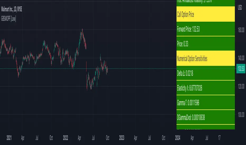
Generalized Black-Scholes-Merton Option Pricing Formula [Loxx]Generalized Black-Scholes-Merton Option Pricing Formula is an adaptation of the Black-Scholes-Merton Option Pricing Model including Numerical Greeks aka "Option Sensitivities" and implied volatility calculations. The following information is an excerpt from Espen Gaarder Haug's book "Option Pricing Formulas".
Black-Scholes-Merton Option Pricing
The BSM formula and its binomial counterpart may easily be the most used "probability model/tool" in everyday use — even if we con- sider all other scientific disciplines. Literally tens of thousands of people, including traders, market makers, and salespeople, use option formulas several times a day. Hardly any other area has seen such dramatic growth as the options and derivatives businesses. In this chapter we look at the various versions of the basic option formula. In 1997 Myron Scholes and Robert Merton were awarded the Nobel Prize (The Bank of Sweden Prize in Economic Sciences in Memory of Alfred Nobel). Unfortunately, Fischer Black died of cancer in 1995 before he also would have received the prize.
It is worth mentioning that it was not the option formula itself that Myron Scholes and Robert Merton were awarded the Nobel Prize for, the formula was actually already invented, but rather for the way they derived it — the replicating portfolio argument, continuous- time dynamic delta hedging, as well as making the formula consistent with the capital asset pricing model (CAPM). The continuous dynamic replication argument is unfortunately far from robust. The popularity among traders for using option formulas heavily relies on hedging options with options and on the top of this dynamic delta hedging, see Higgins (1902), Nelson (1904), Mello and Neuhaus (1998), Derman and Taleb (2005), as well as Haug (2006) for more details on this topic. In any case, this book is about option formulas and not so much about how to derive them.
Provided here are the various versions of the Black-Scholes-Merton formula presented in the literature. All formulas in this section are originally derived based on the underlying asset S follows a geometric Brownian motion
dS = mu * S * dt + v * S * dz
where t is the expected instantaneous rate of return on the underlying asset, a is the instantaneous volatility of the rate of return, and dz is a Wiener process.
The formula derived by Black and Scholes (1973) can be used to value a European option on a stock that does not pay dividends before the option's expiration date. Letting c and p denote the price of European call and put options, respectively, the formula states that
c = S * N(d1) - X * e^(-r * T) * N(d2)
p = X * e^(-r * T) * N(d2) - S * N(d1)
where
d1 = (log(S / X) + (r + v^2 / 2) * T) / (v * T^0.5)
d2 = (log(S / X) + (r - v^2 / 2) * T) / (v * T^0.5) = d1 - v * T^0.5
Inputs
S = Stock price.
X = Strike price of option.
T = Time to expiration in years.
r = Risk-free rate
b = Cost of carry
v = Volatility of the underlying asset price
cnd (x) = The cumulative normal distribution function
nd(x) = The standard normal density function
convertingToCCRate(r, cmp ) = Rate compounder
gImpliedVolatilityNR(string CallPutFlag, float S, float x, float T, float r, float b, float cm, float epsilon) = Implied volatility via Newton Raphson
gBlackScholesImpVolBisection(string CallPutFlag, float S, float x, float T, float r, float b, float cm) = implied volatility via bisection
Implied Volatility: The Bisection Method
The Newton-Raphson method requires knowledge of the partial derivative of the option pricing formula with respect to volatility (vega) when searching for the implied volatility. For some options (exotic and American options in particular), vega is not known analytically. The bisection method is an even simpler method to estimate implied volatility when vega is unknown. The bisection method requires two initial volatility estimates (seed values):
1. A "low" estimate of the implied volatility, al, corresponding to an option value, CL
2. A "high" volatility estimate, aH, corresponding to an option value, CH
The option market price, Cm, lies between CL and cH. The bisection estimate is given as the linear interpolation between the two estimates:
v(i + 1) = v(L) + (c(m) - c(L)) * (v(H) - v(L)) / (c(H) - c(L))
Replace v(L) with v(i + 1) if c(v(i + 1)) < c(m), or else replace v(H) with v(i + 1) if c(v(i + 1)) > c(m) until |c(m) - c(v(i + 1))| <= E, at which point v(i + 1) is the implied volatility and E is the desired degree of accuracy.
Implied Volatility: Newton-Raphson Method
The Newton-Raphson method is an efficient way to find the implied volatility of an option contract. It is nothing more than a simple iteration technique for solving one-dimensional nonlinear equations (any introductory textbook in calculus will offer an intuitive explanation). The method seldom uses more than two to three iterations before it converges to the implied volatility. Let
v(i + 1) = v(i) + (c(v(i)) - c(m)) / (dc / dv(i))
until |c(m) - c(v(i + 1))| <= E at which point v(i + 1) is the implied volatility, E is the desired degree of accuracy, c(m) is the market price of the option, and dc/dv(i) is the vega of the option evaluaated at v(i) (the sensitivity of the option value for a small change in volatility).
Numerical Greeks or Greeks by Finite Difference
Analytical Greeks are the standard approach to estimating Delta, Gamma etc... That is what we typically use when we can derive from closed form solutions. Normally, these are well-defined and available in text books. Previously, we relied on closed form solutions for the call or put formulae differentiated with respect to the Black Scholes parameters. When Greeks formulae are difficult to develop or tease out, we can alternatively employ numerical Greeks - sometimes referred to finite difference approximations. A key advantage of numerical Greeks relates to their estimation independent of deriving mathematical Greeks. This could be important when we examine American options where there may not technically exist an exact closed form solution that is straightforward to work with. (via VinegarHill FinanceLabs)
Things to know
Only works on the daily timeframe and for the current source price.
You can adjust the text size to fit the screen
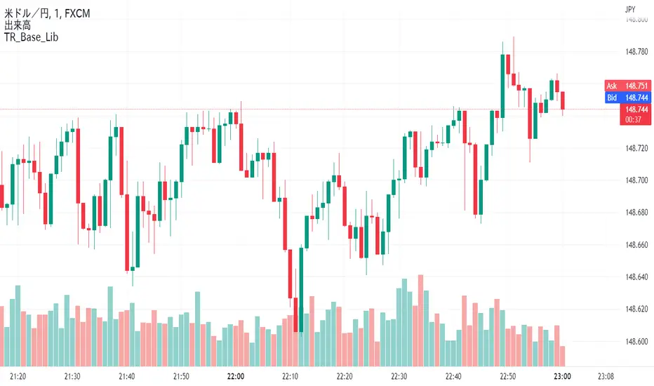
TR_Base_LibLibrary "TR_Base_Lib"
TODO: add library description here
SetHighLowArray()
ChangeHighLowArray()
ShowLabel(_Text, _X, _Y, _Style, _Size, _Yloc, _Color)
TODO: Function to display labels
Parameters:
_Text : TODO: text (series string) Label text.
_X : TODO: x (series int) Bar index.
_Y : TODO: y (series int/float) Price of the label position.
_Style : TODO: style (series string) Label style.
_Size : TODO: size (series string) Label size.
_Yloc : TODO: yloc (series string) Possible values are yloc.price, yloc.abovebar, yloc.belowbar.
_Color : TODO: color (series color) Color of the label border and arrow
Returns: TODO: No return values
GetColor(_Index)
TODO: Function to take out 12 colors in order
Parameters:
_Index : TODO: color number.
Returns: TODO: color code
Tbl_position(_Pos)
TODO: Table display position function
Parameters:
_Pos : TODO: position.
Returns: TODO: Table position
Tbl_position_JP(_Pos)
TODO: テーブル表示位置 日本語表示位置を定数に変換
Parameters:
_Pos : TODO: 日本語表示位置
Returns: TODO: _result:表示位置の定数を返す
TfInMinutes(_Tf)
TODO: 足変換、TimeFrameを分に変換
Parameters:
_Tf : TODO: TimeFrame文字
Returns: TODO: _result:TimeFrameを分に変換した値、_chartTf:チャートのTimeFrameを分に変換した値
TfName_JP(_tf)
TODO: TimeFrameを日本語足名に変換して返す関数 引数がブランクの時はチャートの日本語足名を返す
Parameters:
_tf : TODO: TimeFrame文字
Returns: TODO: _result:日本語足名
DeleteLine()
TODO: Delete Line
Parameters:
: TODO: No parameter
Returns: TODO: No return value
DeleteLabel()
TODO: Delete Label
Parameters:
: TODO: No parameter
Returns: TODO: No return value
TR_HighLow_LibLibrary "TR_HighLow_Lib"
TODO: add library description here
ShowLabel(_Text, _X, _Y, _Style, _Size, _Yloc, _Color)
TODO: Function to display labels
Parameters:
_Text : TODO: text (series string) Label text.
_X : TODO: x (series int) Bar index.
_Y : TODO: y (series int/float) Price of the label position.
_Style : TODO: style (series string) Label style.
_Size : TODO: size (series string) Label size.
_Yloc : TODO: yloc (series string) Possible values are yloc.price, yloc.abovebar, yloc.belowbar.
_Color : TODO: color (series color) Color of the label border and arrow
Returns: TODO: No return values
GetColor(_Index)
TODO: Function to take out 12 colors in order
Parameters:
_Index : TODO: color number.
Returns: TODO: color code
Tbl_position(_Pos)
TODO: Table display position function
Parameters:
_Pos : TODO: position.
Returns: TODO: Table position
DeleteLine()
TODO: Delete Line
Parameters:
: TODO: No parameter
Returns: TODO: No return value
DeleteLabel()
TODO: Delete Label
Parameters:
: TODO: No parameter
Returns: TODO: No return value
ZigZag(_a_PHiLo, _a_IHiLo, _a_FHiLo, _a_DHiLo, _Histories, _Provisional_PHiLo, _Provisional_IHiLo, _Color1, _Width1, _Color2, _Width2, _ShowLabel, _ShowHighLowBar, _HighLowBarWidth, _HighLow_LabelSize)
TODO: Draw a zig-zag line.
Parameters:
_a_PHiLo : TODO: High-Low price array
_a_IHiLo : TODO: High-Low INDEX array
_a_FHiLo : TODO: High-Low flag array sequence 1:High 2:Low
_a_DHiLo : TODO: High-Low Price Differential Array
_Histories : TODO: Array size (High-Low length)
_Provisional_PHiLo : TODO: Provisional High-Low Price
_Provisional_IHiLo : TODO: Provisional High-Low INDEX
_Color1 : TODO: Normal High-Low color
_Width1 : TODO: Normal High-Low width
_Color2 : TODO: Provisional High-Low color
_Width2 : TODO: Provisional High-Low width
_ShowLabel : TODO: Label display flag True: Displayed False: Not displayed
_ShowHighLowBar : TODO: High-Low bar display flag True:Show False:Hide
_HighLowBarWidth : TODO: High-Low bar width
_HighLow_LabelSize : TODO: Label Size
Returns: TODO: No return value
TrendLine(_a_PHiLo, _a_IHiLo, _Histories, _MultiLine, _StartWidth, _EndWidth, _IncreWidth, _StartTrans, _EndTrans, _IncreTrans, _ColorMode, _Color1_1, _Color1_2, _Color2_1, _Color2_2, _Top_High, _Top_Low, _Bottom_High, _Bottom_Low)
TODO: Draw a Trend Line
Parameters:
_a_PHiLo : TODO: High-Low price array
_a_IHiLo : TODO: High-Low INDEX array
_Histories : TODO: Array size (High-Low length)
_MultiLine : TODO: Draw a multiple Line.
_StartWidth : TODO: Line width start value
_EndWidth : TODO: Line width end value
_IncreWidth : TODO: Line width increment value
_StartTrans : TODO: Transparent rate start value
_EndTrans : TODO: Transparent rate finally
_IncreTrans : TODO: Transparent rate increase value
_ColorMode : TODO: 0:Nomal 1:Gradation
_Color1_1 : TODO: Gradation Color 1_1
_Color1_2 : TODO: Gradation Color 1_2
_Color2_1 : TODO: Gradation Color 2_1
_Color2_2 : TODO: Gradation Color 2_2
_Top_High : TODO: _Top_High Value for Gradation
_Top_Low : TODO: _Top_Low Value for Gradation
_Bottom_High : TODO: _Bottom_High Value for Gradation
_Bottom_Low : TODO: _Bottom_Low Value for Gradation
Returns: TODO: No return value
Fibonacci(_a_Fibonacci, _a_PHiLo, _Provisional_PHiLo, _Index, _FrontMargin, _BackMargin)
TODO: Draw a Fibonacci line
Parameters:
_a_Fibonacci : TODO: Fibonacci Percentage Array
_a_PHiLo : TODO: High-Low price array
_Provisional_PHiLo : TODO: Provisional High-Low price (when _Index is 0)
_Index : TODO: Where to draw the Fibonacci line
_FrontMargin : TODO: Fibonacci line front-margin
_BackMargin : TODO: Fibonacci line back-margin
Returns: TODO: No return value
Fibonacci(_a_Fibonacci, _a_PHiLo, _Provisional_PHiLo, _Index1, _FrontMargin1, _BackMargin1, _Transparent1, _Index2, _FrontMargin2, _BackMargin2, _Transparent2)
TODO: Draw a Fibonacci line
Parameters:
_a_Fibonacci : TODO: Fibonacci Percentage Array
_a_PHiLo : TODO: High-Low price array
_Provisional_PHiLo : TODO: Provisional High-Low price (when _Index is 0)
_Index1 : TODO: Where to draw the Fibonacci line 1
_FrontMargin1 : TODO: Fibonacci line front-margin 1
_BackMargin1 : TODO: Fibonacci line back-margin 1
_Transparent1 : TODO: Transparent rate 1
_Index2 : TODO: Where to draw the Fibonacci line 2
_FrontMargin2 : TODO: Fibonacci line front-margin 2
_BackMargin2 : TODO: Fibonacci line back-margin 2
_Transparent2 : TODO: Transparent rate 2
Returns: TODO: No return value
High_Low_Judgment(_Length, _Extension, _Difference)
TODO: Judges High-Low
Parameters:
_Length : TODO: High-Low Confirmation Length
_Extension : TODO: Length of extension when the difference did not open
_Difference : TODO: Difference size
Returns: TODO: _HiLo=High-Low flag 0:Neither high nor low、1:High、2:Low、3:High-Low
_PHi=high price、_PLo=low price、_IHi=High Price Index、_ILo=Low Price Index、
_Cnt=count、_ECnt=Extension count、
_DiffHi=Difference from Start(High)、_DiffLo=Difference from Start(Low)、
_StartHi=Start value(High)、_StartLo=Start value(Low)
High_Low_Data_AddedAndUpdated(_HiLo, _Histories, _PHi, _PLo, _IHi, _ILo, _DiffHi, _DiffLo, _a_PHiLo, _a_IHiLo, _a_FHiLo, _a_DHiLo)
TODO: Adds and updates High-Low related arrays from given parameters
Parameters:
_HiLo : TODO: High-Low flag
_Histories : TODO: Array size (High-Low length)
_PHi : TODO: Price Hi
_PLo : TODO: Price Lo
_IHi : TODO: Index Hi
_ILo : TODO: Index Lo
_DiffHi : TODO: Difference in High
_DiffLo : TODO: Difference in Low
_a_PHiLo : TODO: High-Low price array
_a_IHiLo : TODO: High-Low INDEX array
_a_FHiLo : TODO: High-Low flag array 1:High 2:Low
_a_DHiLo : TODO: High-Low Price Differential Array
Returns: TODO: _PHiLo price array、_IHiLo indexed array、_FHiLo flag array、_DHiLo price-matching array、
Provisional_PHiLo Provisional price、Provisional_IHiLo 暫定インデックス
High_Low(_a_PHiLo, _a_IHiLo, _a_FHiLo, _a_DHiLo, _a_Fibonacci, _Length, _Extension, _Difference, _Histories, _ShowZigZag, _ZigZagColor1, _ZigZagWidth1, _ZigZagColor2, _ZigZagWidth2, _ShowZigZagLabel, _ShowHighLowBar, _ShowTrendLine, _TrendMultiLine, _TrendStartWidth, _TrendEndWidth, _TrendIncreWidth, _TrendStartTrans, _TrendEndTrans, _TrendIncreTrans, _TrendColorMode, _TrendColor1_1, _TrendColor1_2, _TrendColor2_1, _TrendColor2_2, _ShowFibonacci1, _FibIndex1, _FibFrontMargin1, _FibBackMargin1, _FibTransparent1, _ShowFibonacci2, _FibIndex2, _FibFrontMargin2, _FibBackMargin2, _FibTransparent2, _ShowInfoTable1, _TablePosition1, _ShowInfoTable2, _TablePosition2)
TODO: Draw the contents of the High-Low array.
Parameters:
_a_PHiLo : TODO: High-Low price array
_a_IHiLo : TODO: High-Low INDEX array
_a_FHiLo : TODO: High-Low flag sequence 1:High 2:Low
_a_DHiLo : TODO: High-Low Price Differential Array
_a_Fibonacci : TODO: Fibonacci Gnar Matching
_Length : TODO: Length of confirmation
_Extension : TODO: Extension Length of extension when the difference did not open
_Difference : TODO: Difference size
_Histories : TODO: High-Low Length
_ShowZigZag : TODO: ZigZag Display
_ZigZagColor1 : TODO: Colors of ZigZag1
_ZigZagWidth1 : TODO: Width of ZigZag1
_ZigZagColor2 : TODO: Colors of ZigZag2
_ZigZagWidth2 : TODO: Width of ZigZag2
_ShowZigZagLabel : TODO: ZigZagLabel Display
_ShowHighLowBar : TODO: High-Low Bar Display
_ShowTrendLine : TODO: Trend Line Display
_TrendMultiLine : TODO: Trend Multi Line Display
_TrendStartWidth : TODO: Line width start value
_TrendEndWidth : TODO: Line width end value
_TrendIncreWidth : TODO: Line width increment value
_TrendStartTrans : TODO: Starting transmittance value
_TrendEndTrans : TODO: Transmittance End Value
_TrendIncreTrans : TODO: Increased transmittance value
_TrendColorMode : TODO: color mode
_TrendColor1_1 : TODO: Trend Color 1_1
_TrendColor1_2 : TODO: Trend Color 1_2
_TrendColor2_1 : TODO: Trend Color 2_1
_TrendColor2_2 : TODO: Trend Color 2_2
_ShowFibonacci1 : TODO: Fibonacci1 Display
_FibIndex1 : TODO: Fibonacci1 Index No.
_FibFrontMargin1 : TODO: Fibonacci1 Front margin
_FibBackMargin1 : TODO: Fibonacci1 Back Margin
_FibTransparent1 : TODO: Fibonacci1 Transmittance
_ShowFibonacci2 : TODO: Fibonacci2 Display
_FibIndex2 : TODO: Fibonacci2 Index No.
_FibFrontMargin2 : TODO: Fibonacci2 Front margin
_FibBackMargin2 : TODO: Fibonacci2 Back Margin
_FibTransparent2 : TODO: Fibonacci2 Transmittance
_ShowInfoTable1 : TODO: InfoTable1 Display
_TablePosition1 : TODO: InfoTable1 position
_ShowInfoTable2 : TODO: InfoTable2 Display
_TablePosition2 : TODO: InfoTable2 position
Returns: TODO: 無し

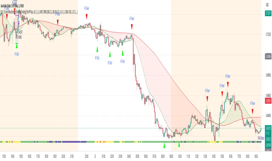
3LS | 3 Line Strike Strategy [Kintsugi Trading]What is the 3LS | 3 Line Strike Strategy?
Incorporating the 3 Line Strike candlestick pattern into our strategy was inspired by Arty at The Moving Average and the amazing traders at TheTrdFloor .
The Three Line Strike is a trend continuation candlestick pattern consisting of four candles. Depending on their heights and collocation, a bullish or a bearish trend continuation can be predicted.
In a symphony of trend analysis, price action, and volume we can find and place high-probability trades with the 3LS Strategy.
How to use it!
----- First, start by choosing a Stop-Loss Strategy, Stop PIP Size, and Risk/Reward Ratio -----
- Stop-Loss Strategy
Fixed PIP Size – This uses the top/bottom of the indicator candle and places a TP based on the chosen Risk:Reward ratio.
ATR Trail (No set Target Profit, only uses ATR Stop)
ATR Trail-Stop (Has set Target Profit, however, stop is based on ATR inputs)
**If you choose an ATR Stop-Loss Strategy - input the desired ATR period and Multiple you would like the stop to be calculated at**
**ATR Stop-Loss Strategies have a unique alert setup for Auto-Trading. See Auto-Trading Section**
- Risk/Reward Ratio = If you have a .5 risk/reward, it means you are risking $100 to make $50.
- Additional Stop PIP Size = Number of PIPs over the default stop location of the top or bottom of the indicator candle.
----- Next, we set the Session Filter -----
Set the Timezone and Trade Session you desire. If no specific session is desired, simply set the Trade Session to 00:00 - 00:00.
----- Next, we set the Moving Average Cloud Fill -----
Enter the Fast and Slow Moving Average Length used to calculate trend direction:
MA Period Fast
MA Period Slow
These inputs will determine whether the strategy looks for Long or Short positions.
----- Next, we set the VSA – Volume Spread Analysis Settings -----
Check the box to show the indicator at the bottom of the chart if desired.
This is just a different visual output of the VSA | Volume Spread Analysis indicator available for free under the community indicators tab. You can add that indicator to your chart and see the same output in candle format.
In combination with the Moving Average Cloud, the Volume Spread Analysis will help us determine when to take a trade and in what direction.
The strategy is essentially looking for small reversals going against the overall trend and placing a trade once that reversal ends and the price moves back in the direction of the overall trend.
The 3LS Strategy utilizes confirmation between trend, volume, and price action to place high probability trades.
The VSA is completely customizable by:
Moving Average Length
MA-1 Multiplier
MA-2 Multiplier
MA-3 Multiplier
Check out the VSA | Volume Spread Analysis indicator in the community scripts section under the indicators tab to use this awesome resource on other strategies.
----- Next, we have the option to view the automated KT Bull/Bear Signals -----
Check the boxes to show the buy-sell signal on the chart if desired.
----- Next, we set the risk we want to use if Auto Trading the strategy -----
I always suggest using no more than 1-3% of your total account balance per trade. Remember, if you have multiple strategies triggering per day with each using 1%, the total percent at risk will be much larger.
For Example – if you have 10 strategies each risking 1% your total risk is 10% of your account, not 1%! Be mindful to only use 1-3% of your total account balance across all strategies, not just each individual one.
----- Finally, we backtest our ideas -----
After using the 'Strategy Tester' tab on TradingView to thoroughly backtest your predictions you are ready to take it to the next level - Automated Trading!
This was my whole reason for creating the script. If you work a full-time job, live in a time zone that is hard to trade, or just don't have the patience, this will be a game-changer for you as it was for me.
Auto-Trading
When it comes to auto-trading this strategy I have included two options in the script that utilize the alert messages generated by TradingView.
*Note: Please trade on a demo account until you feel comfortable enough to use real money, and then please stick to 1%-2% of your total account value in risk per trade.*
AutoView
PineConnector
**ATR Auto-Trading Alert Setup**
How to create alerts on 3 Line Strike Strategy
For Trailing Stops:
1) Adjust autoview/pineconnector settings
2) Click "add alert"
3) Select "Condition" = Strategy Name
4) Select "Order Fills Only" from the drop-down
3) Remove template message text from "message" box and place the exact text. '{{strategy.order.alert_message}}'
4) Click "create"
For Fixed Pip Stop:
1) Adjust autoview/pineconnector settings
2) Click "add alert"
3) Select "Condition" = Strategy Name
4) Select "alert() function calls only"
5) I like to title my Alert Name the same thing I named it as an Indicator Template to keep track
Good luck with your trading!
TR_HighLowLibrary "TR_HighLow"
TODO: add library description here
ShowLabel(_Text, _X, _Y, _Style, _Size, _Yloc, _Color)
TODO: Function to display labels
Parameters:
_Text : TODO: text (series string) Label text.
_X : TODO: x (series int) Bar index.
_Y : TODO: y (series int/float) Price of the label position.
_Style : TODO: style (series string) Label style.
_Size : TODO: size (series string) Label size.
_Yloc : TODO: yloc (series string) Possible values are yloc.price, yloc.abovebar, yloc.belowbar.
_Color : TODO: color (series color) Color of the label border and arrow
Returns: TODO: No return values
GetColor(_Index)
TODO: Function to take out 12 colors in order
Parameters:
_Index : TODO: color number.
Returns: TODO: color code
Tbl_position(_Pos)
TODO: Table display position function
Parameters:
_Pos : TODO: position.
Returns: TODO: Table position
DeleteLine()
TODO: Delete Line
Parameters:
: TODO: No parameter
Returns: TODO: No return value
DeleteLabel()
TODO: Delete Label
Parameters:
: TODO: No parameter
Returns: TODO: No return value
ZigZag(_a_PHiLo, _a_IHiLo, _a_FHiLo, _a_DHiLo, _Histories, _Provisional_PHiLo, _Provisional_IHiLo, _Color1, _Width1, _Color2, _Width2, _ShowLabel, _ShowHighLowBar, _HighLowBarWidth, _HighLow_LabelSize)
TODO: Draw a zig-zag line.
Parameters:
_a_PHiLo : TODO: High-Low price array
_a_IHiLo : TODO: High-Low INDEX array
_a_FHiLo : TODO: High-Low flag array sequence 1:High 2:Low
_a_DHiLo : TODO: High-Low Price Differential Array
_Histories : TODO: Array size (High-Low length)
_Provisional_PHiLo : TODO: Provisional High-Low Price
_Provisional_IHiLo : TODO: Provisional High-Low INDEX
_Color1 : TODO: Normal High-Low color
_Width1 : TODO: Normal High-Low width
_Color2 : TODO: Provisional High-Low color
_Width2 : TODO: Provisional High-Low width
_ShowLabel : TODO: Label display flag True: Displayed False: Not displayed
_ShowHighLowBar : TODO: High-Low bar display flag True:Show False:Hide
_HighLowBarWidth : TODO: High-Low bar width
_HighLow_LabelSize : TODO: Label Size
Returns: TODO: No return value
TrendLine(_a_PHiLo, _a_IHiLo, _Histories, _MultiLine, _StartWidth, _EndWidth, _IncreWidth, _StartTrans, _EndTrans, _IncreTrans, _ColorMode, _Color1_1, _Color1_2, _Color2_1, _Color2_2, _Top_High, _Top_Low, _Bottom_High, _Bottom_Low)
TODO: Draw a Trend Line
Parameters:
_a_PHiLo : TODO: High-Low price array
_a_IHiLo : TODO: High-Low INDEX array
_Histories : TODO: Array size (High-Low length)
_MultiLine : TODO: Draw a multiple Line.
_StartWidth : TODO: Line width start value
_EndWidth : TODO: Line width end value
_IncreWidth : TODO: Line width increment value
_StartTrans : TODO: Transparent rate start value
_EndTrans : TODO: Transparent rate finally
_IncreTrans : TODO: Transparent rate increase value
_ColorMode : TODO: 0:Nomal 1:Gradation
_Color1_1 : TODO: Gradation Color 1_1
_Color1_2 : TODO: Gradation Color 1_2
_Color2_1 : TODO: Gradation Color 2_1
_Color2_2 : TODO: Gradation Color 2_2
_Top_High : TODO: _Top_High Value for Gradation
_Top_Low : TODO: _Top_Low Value for Gradation
_Bottom_High : TODO: _Bottom_High Value for Gradation
_Bottom_Low : TODO: _Bottom_Low Value for Gradation
Returns: TODO: No return value
Fibonacci(_a_Fibonacci, _a_PHiLo, _Provisional_PHiLo, _Index, _FrontMargin, _BackMargin)
TODO: Draw a Fibonacci line
Parameters:
_a_Fibonacci : TODO: Fibonacci Percentage Array
_a_PHiLo : TODO: High-Low price array
_Provisional_PHiLo : TODO: Provisional High-Low price (when _Index is 0)
_Index : TODO: Where to draw the Fibonacci line
_FrontMargin : TODO: Fibonacci line front-margin
_BackMargin : TODO: Fibonacci line back-margin
Returns: TODO: No return value
Fibonacci(_a_Fibonacci, _a_PHiLo, _Provisional_PHiLo, _Index1, _FrontMargin1, _BackMargin1, _Transparent1, _Index2, _FrontMargin2, _BackMargin2, _Transparent2)
TODO: Draw a Fibonacci line
Parameters:
_a_Fibonacci : TODO: Fibonacci Percentage Array
_a_PHiLo : TODO: High-Low price array
_Provisional_PHiLo : TODO: Provisional High-Low price (when _Index is 0)
_Index1 : TODO: Where to draw the Fibonacci line 1
_FrontMargin1 : TODO: Fibonacci line front-margin 1
_BackMargin1 : TODO: Fibonacci line back-margin 1
_Transparent1 : TODO: Transparent rate 1
_Index2 : TODO: Where to draw the Fibonacci line 2
_FrontMargin2 : TODO: Fibonacci line front-margin 2
_BackMargin2 : TODO: Fibonacci line back-margin 2
_Transparent2 : TODO: Transparent rate 2
Returns: TODO: No return value
High_Low_Judgment(_Length, _Extension, _Difference)
TODO: Judges High-Low
Parameters:
_Length : TODO: High-Low Confirmation Length
_Extension : TODO: Length of extension when the difference did not open
_Difference : TODO: Difference size
Returns: TODO: _HiLo=High-Low flag 0:Neither high nor low、1:High、2:Low、3:High-Low
_PHi=high price、_PLo=low price、_IHi=High Price Index、_ILo=Low Price Index、
_Cnt=count、_ECnt=Extension count、
_DiffHi=Difference from Start(High)、_DiffLo=Difference from Start(Low)、
_StartHi=Start value(High)、_StartLo=Start value(Low)
High_Low_Data_AddedAndUpdated(_HiLo, _Histories, _PHi, _PLo, _IHi, _ILo, _DiffHi, _DiffLo, _a_PHiLo, _a_IHiLo, _a_FHiLo, _a_DHiLo)
TODO: Adds and updates High-Low related arrays from given parameters
Parameters:
_HiLo : TODO: High-Low flag
_Histories : TODO: Array size (High-Low length)
_PHi : TODO: Price Hi
_PLo : TODO: Price Lo
_IHi : TODO: Index Hi
_ILo : TODO: Index Lo
_DiffHi : TODO: Difference in High
_DiffLo : TODO: Difference in Low
_a_PHiLo : TODO: High-Low price array
_a_IHiLo : TODO: High-Low INDEX array
_a_FHiLo : TODO: High-Low flag array 1:High 2:Low
_a_DHiLo : TODO: High-Low Price Differential Array
Returns: TODO: _PHiLo price array、_IHiLo indexed array、_FHiLo flag array、_DHiLo price-matching array、
Provisional_PHiLo Provisional price、Provisional_IHiLo 暫定インデックス
High_Low(_a_PHiLo, _a_IHiLo, _a_FHiLo, _a_DHiLo, _a_Fibonacci, _Length, _Extension, _Difference, _Histories, _ShowZigZag, _ZigZagColor1, _ZigZagWidth1, _ZigZagColor2, _ZigZagWidth2, _ShowZigZagLabel, _ShowHighLowBar, _ShowTrendLine, _TrendMultiLine, _TrendStartWidth, _TrendEndWidth, _TrendIncreWidth, _TrendStartTrans, _TrendEndTrans, _TrendIncreTrans, _TrendColorMode, _TrendColor1_1, _TrendColor1_2, _TrendColor2_1, _TrendColor2_2, _ShowFibonacci1, _FibIndex1, _FibFrontMargin1, _FibBackMargin1, _FibTransparent1, _ShowFibonacci2, _FibIndex2, _FibFrontMargin2, _FibBackMargin2, _FibTransparent2, _ShowInfoTable1, _TablePosition1, _ShowInfoTable2, _TablePosition2)
TODO: Draw the contents of the High-Low array.
Parameters:
_a_PHiLo : TODO: High-Low price array
_a_IHiLo : TODO: High-Low INDEX array
_a_FHiLo : TODO: High-Low flag sequence 1:High 2:Low
_a_DHiLo : TODO: High-Low Price Differential Array
_a_Fibonacci : TODO: Fibonacci Gnar Matching
_Length : TODO: Length of confirmation
_Extension : TODO: Extension Length of extension when the difference did not open
_Difference : TODO: Difference size
_Histories : TODO: High-Low Length
_ShowZigZag : TODO: ZigZag Display
_ZigZagColor1 : TODO: Colors of ZigZag1
_ZigZagWidth1 : TODO: Width of ZigZag1
_ZigZagColor2 : TODO: Colors of ZigZag2
_ZigZagWidth2 : TODO: Width of ZigZag2
_ShowZigZagLabel : TODO: ZigZagLabel Display
_ShowHighLowBar : TODO: High-Low Bar Display
_ShowTrendLine : TODO: Trend Line Display
_TrendMultiLine : TODO: Trend Multi Line Display
_TrendStartWidth : TODO: Line width start value
_TrendEndWidth : TODO: Line width end value
_TrendIncreWidth : TODO: Line width increment value
_TrendStartTrans : TODO: Starting transmittance value
_TrendEndTrans : TODO: Transmittance End Value
_TrendIncreTrans : TODO: Increased transmittance value
_TrendColorMode : TODO: color mode
_TrendColor1_1 : TODO: Trend Color 1_1
_TrendColor1_2 : TODO: Trend Color 1_2
_TrendColor2_1 : TODO: Trend Color 2_1
_TrendColor2_2 : TODO: Trend Color 2_2
_ShowFibonacci1 : TODO: Fibonacci1 Display
_FibIndex1 : TODO: Fibonacci1 Index No.
_FibFrontMargin1 : TODO: Fibonacci1 Front margin
_FibBackMargin1 : TODO: Fibonacci1 Back Margin
_FibTransparent1 : TODO: Fibonacci1 Transmittance
_ShowFibonacci2 : TODO: Fibonacci2 Display
_FibIndex2 : TODO: Fibonacci2 Index No.
_FibFrontMargin2 : TODO: Fibonacci2 Front margin
_FibBackMargin2 : TODO: Fibonacci2 Back Margin
_FibTransparent2 : TODO: Fibonacci2 Transmittance
_ShowInfoTable1 : TODO: InfoTable1 Display
_TablePosition1 : TODO: InfoTable1 position
_ShowInfoTable2 : TODO: InfoTable2 Display
_TablePosition2 : TODO: InfoTable2 position
Returns: TODO: 無し

Webhook Starter Kit [HullBuster]
Introduction
This is an open source strategy which provides a framework for webhook enabled projects. It is designed to work out-of-the-box on any instrument triggering on an intraday bar interval. This is a full featured script with an emphasis on actual trading at a brokerage through the TradingView alert mechanism and without requiring browser plugins.
The source code is written in a self documenting style with clearly defined sections. The sections “communicate” with each other through state variables making it easy for the strategy to evolve and improve. This is an excellent place for Pine Language beginners to start their strategy building journey. The script exhibits many Pine Language features which will certainly ad power to your script building abilities.
This script employs a basic trend follow strategy utilizing a forward pyramiding technique. Trend detection is implemented through the use of two higher time frame series. The market entry setup is a Simple Moving Average crossover. Positions exit by passing through conditional take profit logic. The script creates ten indicators including a Zscore oscillator to measure support and resistance levels. The indicator parameters are exposed through 47 strategy inputs segregated into seven sections. All of the inputs are equipped with detailed tool tips to help you get started.
To improve the transition from simulation to execution, strategy.entry and strategy.exit calls show enhanced message text with embedded keywords that are combined with the TradingView placeholders at alert time. Thereby, enabling a single JSON message to generate multiple execution events. This is genius stuff from the Pine Language development team. Really excellent work!
This document provides a sample alert message that can be applied to this script with relatively little modification. Without altering the code, the strategy inputs can alter the behavior to generate thousands of orders or simply a few dozen. It can be applied to crypto, stocks or forex instruments. A good way to look at this script is as a webhook lab that can aid in the development of your own endpoint processor, impress your co-workers and have hours of fun.
By no means is a webhook required or even necessary to benefit from this script. The setups, exits, trend detection, pyramids and DCA algorithms can be easily replaced with more sophisticated versions. The modular design of the script logic allows you to incrementally learn and advance this script into a functional trading system that you can be proud of.
Design
This is a trend following strategy that enters long above the trend line and short below. There are five trend lines that are visible by default but can be turned off in Section 7. Identified, in frequency order, as follows:
1. - EMA in the chart time frame. Intended to track price pressure. Configured in Section 3.
2. - ALMA in the higher time frame specified in Section 2 Signal Line Period.
3. - Linear Regression in the higher time frame specified in Section 2 Signal Line Period.
4. - Linear Regression in the higher time frame specified in Section 2 Signal Line Period.
5. - DEMA in the higher time frame specified in Section 2 Trend Line Period.
The Blue, Green and Orange lines are signal lines are on the same time frame. The time frame selected should be at least five times greater than the chart time frame. The Purple line represents the trend line for which prices above the line suggest a rising market and prices below a falling market. The time frame selected for the trend should be at least five times greater than the signal lines.
Three oscillators are created as follows:
1. Stochastic - In the chart time frame. Used to enter forward pyramids.
2. Stochastic - In the Trend period. Used to detect exit conditions.
3. Zscore - In the Signal period. Used to detect exit conditions.
The Stochastics are configured identically other than the time frame. The period is set in Section 2.
Two Simple Moving Averages provide the trade entry conditions in the form of a crossover. Crossing up is a long entry and down is a short. This is in fact the same setup you get when you select a basic strategy from the Pine editor. The crossovers are configured in Section 3. You can see where the crosses are occurring by enabling Show Entry Regions in Section 7.
The script has the capacity for pyramids and DCA. Forward pyramids are enabled by setting the Pyramid properties tab with a non zero value. In this case add on trades will enter the market on dips above the position open price. This process will continue until the trade exits. Downward pyramids are available in Crypto and Range mode only. In this case add on trades are placed below the entry price in the drawdown space until the stop is hit. To enable downward pyramids set the Pyramid Minimum Span In Section 1 to a non zero value.
This implementation of Dollar Cost Averaging (DCA) triggers off consecutive losses. Each loss in a run increments a sequence number. The position size is increased as a multiple of this sequence. When the position eventually closes at a profit the sequence is reset. DCA is enabled by setting the Maximum DCA Increments In Section 1 to a non zero value.
It should be noted that the pyramid and DCA features are implemented using a rudimentary design and as such do not perform with the precision of my invite only scripts. They are intended as a feature to stress test your webhook endpoint. As is, you will need to buttress the logic for it to be part of an automated trading system. It is for this reason that I did not apply a Martingale algorithm to this pyramid implementation. But, hey, it’s an open source script so there is plenty of room for learning and your own experimentation.
How does it work
The overall behavior of the script is governed by the Trading Mode selection in Section 1. It is the very first input so you should think about what behavior you intend for this strategy at the onset of the configuration. As previously discussed, this script is designed to be a trend follower. The trend being defined as where the purple line is predominately heading. In BiDir mode, SMA crossovers above the purple line will open long positions and crosses below the line will open short. If pyramiding is enabled add on trades will accumulate on dips above the entry price. The value applied to the Minimum Profit input in Section 1 establishes the threshold for a profitable exit. This is not a hard number exit. The conditional exit logic must be satisfied in order to permit the trade to close. This is where the effort put into the indicator calibration is realized. There are four ways the trade can exit at a profit:
1. Natural exit. When the blue line crosses the green line the trade will close. For a long position the blue line must cross under the green line (downward). For a short the blue must cross over the green (upward).
2. Alma / Linear Regression event. The distance the blue line is from the green and the relative speed the cross is experiencing determines this event. The activation thresholds are set in Section 6 and relies on the period and length set in Section 2. A long position will exit on an upward thrust which exceeds the activation threshold. A short will exit on a downward thrust.
3. Exponential event. The distance the yellow line is from the blue and the relative speed the cross is experiencing determines this event. The activation thresholds are set in Section 3 and relies on the period and length set in the same section.
4. Stochastic event. The purple line stochastic is used to measure overbought and over sold levels with regard to position exits. Signal line positions combined with a reading over 80 signals a long profit exit. Similarly, readings below 20 signal a short profit exit.
Another, optional, way to exit a position is by Bale Out. You can enable this feature in Section 1. This is a handy way to reduce the risk when carrying a large pyramid stack. Instead of waiting for the entire position to recover we exit early (bale out) as soon as the profit value has doubled.
There are lots of ways to implement a bale out but the method I used here provides a succinct example. Feel free to improve on it if you like. To see where the Bale Outs occur, enable Show Bale Outs in Section 7. Red labels are rendered below each exit point on the chart.
There are seven selectable Trading Modes available from the drop down in Section 1:
1. Long - Uses the strategy.risk.allow_entry_in to execute long only trades. You will still see shorts on the chart.
2. Short - Uses the strategy.risk.allow_entry_in to execute short only trades. You will still see long trades on the chart.
3. BiDir - This mode is for margin trading with a stop. If a long position was initiated above the trend line and the price has now fallen below the trend, the position will be reversed after the stop is hit. Forward pyramiding is available in this mode if you set the Pyramiding value in the Properties tab. DCA can also be activated.
4. Flip Flop - This is a bidirectional trading mode that automatically reverses on a trend line crossover. This is distinctively different from BiDir since you will get a reversal even without a stop which is advantageous in non-margin trading.
5. Crypto - This mode is for crypto trading where you are buying the coins outright. In this case you likely want to accumulate coins on a crash. Especially, when all the news outlets are talking about the end of Bitcoin and you see nice deep valleys on the chart. Certainly, under these conditions, the market will be well below the purple line. No margin so you can’t go short. Downward pyramids are enabled for Crypto mode when two conditions are met. First the Pyramiding value in the Properties tab must be non zero. Second the Pyramid Minimum Span in Section 1 must be non zero.
6. Range - This is a counter trend trading mode. Longs are entered below the purple trend line and shorts above. Useful when you want to test your webhook in a market where the trend line is bisecting the signal line series. Remember that this strategy is a trend follower. It’s going to get chopped out in a range bound market. By turning on the Range mode you will at least see profitable trades while stuck in the range. However, when the market eventually picks a direction, this mode will sustain losses. This range trading mode is a rudimentary implementation that will need a lot of improvement if you want to create a reliable switch hitter (trend/range combo).
7. No Trade. Useful when setting up the trend lines and the entry and exit is not important.
Once in the trade, long or short, the script tests the exit condition on every bar. If not a profitable exit then it checks if a pyramid is required. As mentioned earlier, the entry setups are quite primitive. Although they can easily be replaced by more sophisticated algorithms, what I really wanted to show is the diminished role of the position entry in the overall life of the trade. Professional traders spend much more time on the management of the trade beyond the market entry. While your trade entry is important, you can get in almost anywhere and still land a profitable exit.
If DCA is enabled, the size of the position will increase in response to consecutive losses. The number of times the position can increase is limited by the number set in Maximum DCA Increments of Section 1. Once the position breaks the losing streak the trade size will return the default quantity set in the Properties tab. It should be noted that the Initial Capital amount set in the Properties tab does not affect the simulation in the same way as a real account. In reality, running out of money will certainly halt trading. In fact, your account would be frozen long before the last penny was committed to a trade. On the other hand, TradingView will keep running the simulation until the current bar even if your funds have been technically depleted.
Entry and exit use the strategy.entry and strategy.exit calls respectfully. The alert_message parameter has special keywords that the endpoint expects to properly calculate position size and message sequence. The alert message will embed these keywords in the JSON object through the {{strategy.order.alert_message}} placeholder. You should use whatever keywords are expected from the endpoint you intend to webhook in to.
Webhook Integration
The TradingView alerts dialog provides a way to connect your script to an external system which could actually execute your trade. This is a fantastic feature that enables you to separate the data feed and technical analysis from the execution and reporting systems. Using this feature it is possible to create a fully automated trading system entirely on the cloud. Of course, there is some work to get it all going in a reliable fashion. Being a strategy type script place holders such as {{strategy.position_size}} can be embedded in the alert message text. There are more than 10 variables which can write internal script values into the message for delivery to the specified endpoint.
Entry and exit use the strategy.entry and strategy.exit calls respectfully. The alert_message parameter has special keywords that my endpoint expects to properly calculate position size and message sequence. The alert message will embed these keywords in the JSON object through the {{strategy.order.alert_message}} placeholder. You should use whatever keywords are expected from the endpoint you intend to webhook in to.
Here is an excerpt of the fields I use in my webhook signal:
"broker_id": "kraken",
"account_id": "XXX XXXX XXXX XXXX",
"symbol_id": "XMRUSD",
"action": "{{strategy.order.action}}",
"strategy": "{{strategy.order.id}}",
"lots": "{{strategy.order.contracts}}",
"price": "{{strategy.order.price}}",
"comment": "{{strategy.order.alert_message}}",
"timestamp": "{{time}}"
Though TradingView does a great job in dispatching your alert this feature does come with a few idiosyncrasies. Namely, a single transaction call in your script may cause multiple transmissions to the endpoint. If you are using placeholders each message describes part of the transaction sequence. A good example is closing a pyramid stack. Although the script makes a single strategy.close() call, the endpoint actually receives a close message for each pyramid trade. The broker, on the other hand, only requires a single close. The incongruity of this situation is exacerbated by the possibility of messages being received out of sequence. Depending on the type of order designated in the message, a close or a reversal. This could have a disastrous effect on your live account. This broker simulator has no idea what is actually going on at your real account. Its just doing the job of running the simulation and sending out the computed results. If your TradingView simulation falls out of alignment with the actual trading account lots of really bad things could happen. Like your script thinks your are currently long but the account is actually short. Reversals from this point forward will always be wrong with no one the wiser. Human intervention will be required to restore congruence. But how does anyone find out this is occurring? In closed systems engineering this is known as entropy. In practice your webhook logic should be robust enough to detect these conditions. Be generous with the placeholder usage and give the webhook code plenty of information to compare states. Both issuer and receiver. Don’t blindly commit incoming signals without verifying system integrity.
Setup
The following steps provide a very brief set of instructions that will get you started on your first configuration. After you’ve gone through the process a couple of times, you won’t need these anymore. It’s really a simple script after all. I have several example configurations that I used to create the performance charts shown. I can share them with you if you like. Of course, if you’ve modified the code then these steps are probably obsolete.
There are 47 inputs divided into seven sections. For the most part, the configuration process is designed to flow from top to bottom. Handy, tool tips are available on every field to help get you through the initial setup.
Step 1. Input the Base Currency and Order Size in the Properties tab. Set the Pyramiding value to zero.
Step 2. Select the Trading Mode you intend to test with from the drop down in Section 1. I usually select No Trade until I’ve setup all of the trend lines, profit and stop levels.
Step 3. Put in your Minimum Profit and Stop Loss in the first section. This is in pips or currency basis points (chart right side scale). Remember that the profit is taken as a conditional exit not a fixed limit. The actual profit taken will almost always be greater than the amount specified. The stop loss, on the other hand, is indeed a hard number which is executed by the TradingView broker simulator when the threshold is breached.
Step 4. Apply the appropriate value to the Tick Scalar field in Section 1. This value is used to remove the pipette from the price. You can enable the Summary Report in Section 7 to see the TradingView minimum tick size of the current chart.
Step 5. Apply the appropriate Price Normalizer value in Section 1. This value is used to normalize the instrument price for differential calculations. Basically, we want to increase the magnitude to significant digits to make the numbers more meaningful in comparisons. Though I have used many normalization techniques, I have always found this method to provide a simple and lightweight solution for less demanding applications. Most of the time the default value will be sufficient. The Tick Scalar and Price Normalizer value work together within a single calculation so changing either will affect all delta result values.
Step 6. Turn on the trend line plots in Section 7. Then configure Section 2. Try to get the plots to show you what’s really happening not what you want to happen. The most important is the purple trend line. Select an interval and length that seem to identify where prices tend to go during non-consolidation periods. Remember that a natural exit is when the blue crosses the green line.
Step 7. Enable Show Event Regions in Section 7. Then adjust Section 6. Blue background fills are spikes and red fills are plunging prices. These measurements should be hard to come by so you should see relatively few fills on the chart if you’ve set this up as intended. Section 6 includes the Zscore oscillator the state of which combines with the signal lines to detect statistically significant price movement. The Zscore is a zero based calculation with positive and negative magnitude readings. You want to input a reasonably large number slightly below the maximum amplitude seen on the chart. Both rise and fall inputs are entered as a positive real number. You can easily use my code to create a separate indicator if you want to see it in action. The default value is sufficient for most configurations.
Step 8. Turn off Show Event Regions and enable Show Entry Regions in Section 7. Then adjust Section 3. This section contains two parts. The entry setup crossovers and EMA events. Adjust the crossovers first. That is the Fast Cross Length and Slow Cross Length. The frequency of your trades will be shown as blue and red fills. There should be a lot. Then turn off Show Event Regions and enable Display EMA Peaks. Adjust all the fields that have the word EMA. This is actually the yellow line on the chart. The blue and red fills should show much less than the crossovers but more than event fills shown in Step 7.
Step 9. Change the Trading Mode to BiDir if you selected No Trades previously. Look on the chart and see where the trades are occurring. Make adjustments to the Minimum Profit and Stop Offset in Section 1 if necessary. Wider profits and stops reduce the trade frequency.
Step 10. Go to Section 4 and 5 and make fine tuning adjustments to the long and short side.
Example Settings
To reproduce the performance shown on the chart please use the following configuration: (Bitcoin on the Kraken exchange)
1. Select XBTUSD Kraken as the chart symbol.
2. On the properties tab set the Order Size to: 0.01 Bitcoin
3. On the properties tab set the Pyramiding to: 12
4. In Section 1: Select “Crypto” for the Trading Model
5. In Section 1: Input 2000 for the Minimum Profit
6. In Section 1: Input 0 for the Stop Offset (No Stop)
7. In Section 1: Input 10 for the Tick Scalar
8. In Section 1: Input 1000 for the Price Normalizer
9. In Section 1: Input 2000 for the Pyramid Minimum Span
10. In Section 1: Check mark the Position Bale Out
11. In Section 2: Input 60 for the Signal Line Period
12. In Section 2: Input 1440 for the Trend Line Period
13. In Section 2: Input 5 for the Fast Alma Length
14. In Section 2: Input 22 for the Fast LinReg Length
15. In Section 2: Input 100 for the Slow LinReg Length
16. In Section 2: Input 90 for the Trend Line Length
17. In Section 2: Input 14 Stochastic Length
18. In Section 3: Input 9 Fast Cross Length
19. In Section 3: Input 24 Slow Cross Length
20. In Section 3: Input 8 Fast EMA Length
21. In Section 3: Input 10 Fast EMA Rise NetChg
22. In Section 3: Input 1 Fast EMA Rise ROC
23. In Section 3: Input 10 Fast EMA Fall NetChg
24. In Section 3: Input 1 Fast EMA Fall ROC
25. In Section 4: Check mark the Long Natural Exit
26. In Section 4: Check mark the Long Signal Exit
27. In Section 4: Check mark the Long Price Event Exit
28. In Section 4: Check mark the Long Stochastic Exit
29. In Section 5: Check mark the Short Natural Exit
30. In Section 5: Check mark the Short Signal Exit
31. In Section 5: Check mark the Short Price Event Exit
32. In Section 5: Check mark the Short Stochastic Exit
33. In Section 6: Input 120 Rise Event NetChg
34. In Section 6: Input 1 Rise Event ROC
35. In Section 6: Input 5 Min Above Zero ZScore
36. In Section 6: Input 120 Fall Event NetChg
37. In Section 6: Input 1 Fall Event ROC
38. In Section 6: Input 5 Min Below Zero ZScore
In this configuration we are trading in long only mode and have enabled downward pyramiding. The purple trend line is based on the day (1440) period. The length is set at 90 days so it’s going to take a while for the trend line to alter course should this symbol decide to node dive for a prolonged amount of time. Your trades will still go long under those circumstances. Since downward accumulation is enabled, your position size will grow on the way down.
The performance example is Bitcoin so we assume the trader is buying coins outright. That being the case we don’t need a stop since we will never receive a margin call. New buy signals will be generated when the price exceeds the magnitude and speed defined by the Event Net Change and Rate of Change.
Feel free to PM me with any questions related to this script. Thank you and happy trading!
CFTC RULE 4.41
These results are based on simulated or hypothetical performance results that have certain inherent limitations. Unlike the results shown in an actual performance record, these results do not represent actual trading. Also, because these trades have not actually been executed, these results may have under-or over-compensated for the impact, if any, of certain market factors, such as lack of liquidity. Simulated or hypothetical trading programs in general are also subject to the fact that they are designed with the benefit of hindsight. No representation is being made that any account will or is likely to achieve profits or losses similar to these being shown.

Financials on Chart█ OVERVIEW
This indicator displays your choice of up to 9 fundamentals on your chart.
█ FEATURES
You can configure the following attributes of the display:
• Its position on your chart.
• Automatic or custom height and width of rows.
• The size and color of text.
• The default background color (you can override it with a custom color for individual values).
• Conversion of values expressed in USD to one of the major currencies. Financials are normally expressed in quote currency.
Conversion to other currencies is only done when the symbol's quote currency is USD.
• Choose if the currency used for the financials is displayed. Note that some financials are calculated values that are not expressed in currency units.
No currency will be displayed for these values.
• Abbreviate large values.
For each value, you may:
• Pick one of the 222 financials available in Pine, or one of five values calculated from the financials (Market Cap, Earnings Yield, P/B Ratio, P/E Ratio and Price-To-Sales Ratio).
• Choose a period (see the "i" icon near the first value's fields in the script's inputs for a list of exceptions).
• Specify the value's precision.
• Change the legend displayed with the value.
• Adjust the text's size.
• Use a custom background.
█ LIMITATIONS
When changing the indicator's inputs, allow a few seconds for the change to be reflected in the display.
If your chart displays a symbol for which the configured financials cannot be fetched, an error will occur.
Not all periods are available for all fundamentals or for all markets. What financial data is available in Pine? will give you an overview of the available periods for each value. The page also contains the formulas used for the five values we calculate from the financials. This page shows the typical reporting frequency for different countries .
█ FINANCIALS
See What is Financial Data? and Why does Financial Data differ from other sources? for more information on the data used by this indicator.
This lists all the financials. Clicking on one will bring up more information about it:
CALCULATED
Market Capitalization
Earnings Yield
Price Book Ratio
Price Earnings Ratio
Price-To-Sales Ratio
INCOME STATEMENTS
After tax other income/expense
Average basic shares outstanding
Other COGS
Cost of goods
Deprecation and amortization
Diluted net income available to common stockholders
Diluted shares outstanding
Dilution adjustment
Discontinued operations
Basic EPS
Diluted EPS
EBIT
EBITDA
Equity in earnings
Gross profit
Taxes
Interest capitalized
Interest expense on debt
Non-controlling/minority interest
Net income before discontinued operations
Net income
Non-operating income, excl. interest expenses
Interest expense, net of interest capitalized
Non-operating interest income
Operating income
Operating expenses (excl. COGS)
Miscellaneous non-operating expense
Other operating expenses, total
Preferred dividends
Pretax equity in earnings
Pretax income
Research & development
Selling/general/admin expenses, other
Selling/general/admin expenses, total
Non-operating income, total
Total operating expenses
Total revenue
Unusual income/expense
BALANCE SHEET
Accounts payable
Accounts receivable - trade, net
Accrued payroll
Accumulated depreciation, total
Additional paid-in capital/Capital surplus
Tangible book value per share
Book value per share
Capitalized lease obligations
Capital and operating lease obligations
Cash & equivalents
Cash and short term investments
Common equity, total
Common stock par/Carrying value
Current portion of LT debt and capital leases
Deferred income, current
Deferred income, non-current
Deferred tax assets
Deferred tax liabilities
Dividends payable
Goodwill, net
Income tax payable
Net intangible assets
Inventories - finished goods
Inventories - progress payments & other
Inventories - raw materials
Inventories - work in progress
Investments in unconsolidated subsidiaries
Long term debt excl. lease liabilities
Long term debt
Long term investments
Note receivable - long term
Other long term assets, total
Minority interest
Notes payable
Operating lease liabilities
Other common equity
Other current assets, total
Other current liabilities
Other intangibles, net
Other investments
Other liabilities, total
Other receivables
Other short term debt
Paid in capital
Gross property/plant/equipment
Net property/plant/equipment
Preferred stock, carrying value
Prepaid expenses
Provision for risks & charge
Retained earnings
Short term debt excl. current portion of LT debt
Short term debt
Short term investments
Shareholders' equity
Total assets
Total current assets
Total current liabilities
Total debt
Total equity
Total inventory
Total liabilities
Total liabilities & shareholders' equities
Total non-current assets
Total non-current liabilities
Total receivables, net
Treasury stock - common
CASHFLOW
Amortization
Capital expenditures - fixed assets
Capital expenditures
Capital expenditures - other assets
Cash from financing activities
Cash from investing activities
Cash from operating activities
Deferred taxes (cash flow)
Depreciation & amortization (cash flow)
Change in accounts payable
Change in accounts receivable
Change in accrued expenses
Change in inventories
Change in other assets/liabilities
Change in taxes payable
Changes in working capital
Common dividends paid
Depreciation/depletion
Free cash flow
Funds from operations
Issuance/retirement of debt, net
Issuance/retirement of long term debt
Issuance/retirement of other debt
Issuance/retirement of short term debt
Issuance/retirement of stock, net
Net income (cash flow)
Non-cash items
Other financing cash flow items, total
Financing activities - other sources
Financing activities - other uses
Other investing cash flow items, total
Investing activities - other sources
Investing activities - other uses
Preferred dividends paid
Purchase/acquisition of business
Purchase of investments
Repurchase of common & preferred stock
Purchase/sale of business, net
Purchase/sale of investments, net
Reduction of long term debt
Sale of common & preferred stock
Sale of fixed assets & businesses
Sale/maturity of investments
Issuance of long term debt
Total cash dividends paid
STATISTICS
Accruals
Altman Z-score
Asset turnover
Beneish M-score
Buyback yield %
Cash conversion cycle
Cash to debt ratio
COGS to revenue ratio
Current ratio
Days sales outstanding
Days inventory
Days payable
Debt to assets ratio
Debt to EBITDA ratio
Debt to equity ratio
Debt to revenue ratio
Dividend payout ratio %
Dividend yield %
Dividends per share - common stock primary issue
EPS estimates
EPS basic one year growth
EPS diluted one year growth
EBITDA margin %
Effective interest rate on debt %
Enterprise value to EBITDA ratio
Enterprise value
Equity to assets ratio
Enterprise value to EBIT ratio
Enterprise value to revenue ratio
Float shares outstanding
Free cash flow margin %
Fulmer H factor
Goodwill to assets ratio
Graham's number
Gross margin %
Gross profit to assets ratio
Interest coverage
Inventory to revenue ratio
Inventory turnover
KZ index
Long term debt to total assets ratio
Net current asset value per share
Net income per employee
Net margin %
Number of employees
Operating earnings yield %
Operating margin %
PEG ratio
Piotroski F-score
Price earnings ratio forward
Price sales ratio forward
Price to free cash flow ratio
Price to tangible book ratio
Quality ratio
Quick ratio
Research & development to revenue ratio
Return on assets %
Return on equity adjusted to book value %
Return on equity %
Return on invested capital %
Return on tangible assets %
Return on tangible equity %
Revenue one year growth
Revenue per employee
Revenue estimates
Shares buyback ratio %
Sloan ratio %
Springate score
Sustainable growth rate
Tangible common equity ratio
Tobin's Q (approximate)
Total common shares outstanding
Zmijewski score
█ NOTES
This script uses the Pine financial() function to fetch the values it displays.
Look first. Then leap.

InariN CloudSInariN CloudS (INCS) is my custom model of InariN.
I usually use INCS in 300 ticks (other software) and 5 minutes charts for day trading.
Please read script "InariN simple" for basic usage.
I share background and fundamental ideas of day trading and INCS here.
I start with the practical conclusion and then explain INCS.
Maybe you'll notice that most indicators are unnecessary at the end of this text.
Anyway I compile fundamental ideas that I wanted to know as a beginner.
(I'll update to finish this text, please wait for some time.)
///Premise of trading///
Market's purpose...facilitating trading
Trader's purpose...making money
Market is stronger than trader and trader need adjust to market.
However trader have controllable side.
Market's control...Trend, Volatility
Trader's control...Money management, Making Risk:Reward, Choosing and exercising trading strategy
///Simple rule (Conclusion)///
I made simple rule "Just Do It Now" to check essential ideas on every trade.
Traders can use thousands of indicators but only use three choices "Buy, Sell and No trade".
If you have bad result, you had better suspect not your indicators but your three choices at first.
(This is one of the best advice I have ever heard by N jijii.)

Setup 9.1 by Larry Williams Setup 9.1 by Larry Williams.
The indicator will give text signal and change the color of the signal candle, being based exclusively on the setup 9.1
----------//---------------
PT-BR
Setup 9.1 do Larry Williams.
O indicador irá dar sinal de texto e alterar a cor do candle de sinal, se baseando exclusivamente no setup 9.1

Multi Bar OHLC Compare Panel (Floating Grid)Multi Bar OHLC Compare Panel by RagingRocketBull 2019
version 1.0
This indicator lets you compare OHLCV values from several specified bars. Bars can be dynamic/persistent.
You can also use it as an alternate OHLC panel if you don't like small font of the native TradingView panel.
It uses Pinescript v4 to output data dynamically as string labels in a horiz/vertical grid.
Features:
- Floating Panel with customizable horiz/vertical layout and grid spacing
- Support for up to 5 OHLC bars (highlighted with markers)
- Outputs Bar #/index, OHLCV, Bar Change Value/%, Exchange/Ticker, Timeframe, Timestamp strings
- Dynamic (fixed offset)/Persistent bars (fixed time)
- Show/Hide parts of strings
- Full output string customization, including text size, date/time format and delimiters
- 2 Anchor points for panel offset: cur bar high or range high
- Bar Change can change color
Usage:
- specify at least 1 bar index as OHLC source
- select anchor point to position the panel
- select horiz/vertical grid layout
- adjust horiz/vertical spacing
- customize output strings as needed
Notes:
- this indicator uses Pinescript v3 Compatibity Framework
- both bars 1,2 are required for log scale adjustment to work
- you can't attach the panel to screen's top/bottom and must use offset/anchor because, unlike plotshape, string labels don't support yloc=yloc.top/bottom, only yloc.above/belowbar
- you can't precisely align strings in a grid because there's no label.get_width/height to calculate mid/left points, only get_x/y/text. Alignment will break depending on string length, zoom and change color option on/off
- bar change is rendered as a separate label when change color is enabled (2 panels total) and merged into the main panel when disabled (single panel)
- you can't change the order of strings as playing with the natural order of things isn't the best of ideas
- you can modify the script to compare up to 50 OHLC bars, but do you need that much power? Of course, you do.
- you can't set color/style for string labels in Style UI, so a few extra settings were added.
- bar index is limited to 5000 for free accounts (10000 for paid), will show an error when exceeded, also when it exceeds the total number of bars in history
- in persistent bars mode all bars with index > 0 are considered persistent, bar 0 always remains a dynamic bar
- persistent bars' offset is reset: in replay mode on exit or when price reaches cur bar, or when panel layout is changed from h to v in both replay/realtime modes
- initial pos of each persistent bar relative to the first realtime bar anchor doesn't change during session - new persistent bars introduced during session are attached to the most recent cur bar anchor
P.S. Everything is proceeding as I have foreseen

EXPLOSION Scanner v1 - Sudden Spike Hunter//@version=5
indicator("EXPLOSION ENTRY v1 - 5Day Swing Breakout Scanner", overlay=true)
// ===============================
// 입력값
// ===============================
lenBB = input.int(20, "BB Length")
multBB = input.float(2.0, "BB StdDev")
lenVolMA = input.int(20, "Volume MA Length")
volMult = input.float(1.8, "Volume Explosion Mult")
lenATR = input.int(14, "ATR Length")
atrThresh= input.float(3.0, "ATR % Threshold")
needBull = input.int(4, "최근 5봉 중 최소 양봉 개수", minval=1, maxval=5)
// ===============================
// Bollinger Band
// ===============================
basis = ta.sma(close, lenBB)
dev = ta.stdev(close, lenBB)
upper = basis + dev * multBB
lower = basis - dev * multBB
plot(upper, "BB Upper", display=display.none)
plot(basis, "BB Basis", display=display.none)
plot(lower, "BB Lower", display=display.none)
// ===============================
// Volume Explosion
// ===============================
volMA = ta.sma(volume, lenVolMA)
volCond = volume > volMA * volMult
// ===============================
// 5-Day Candle Strength (최근 5봉 양봉 개수)
// ===============================
bullCount = (close > open ? 1 : 0) +
(close > open ? 1 : 0) +
(close > open ? 1 : 0) +
(close > open ? 1 : 0) +
(close > open ? 1 : 0)
candleCond = bullCount >= needBull
// ===============================
// ATR Volatility Filter
// ===============================
atrValue = ta.atr(lenATR)
atrRate = atrValue / close * 100.0
volatilityCond = atrRate > atrThresh
// ===============================
// Trend Filter (기본 추세)
// ===============================
trendCond = close > basis
// ===============================
// 최종 매수 조건
// ===============================
buyCond = trendCond and volCond and candleCond and volatilityCond
// ===============================
// BUY 신호 표시
// ===============================
plotshape(
buyCond,
title = "BUY Signal",
style = shape.triangleup,
location = location.belowbar,
size = size.small,
text = "BUY",
textcolor = color.white
)
// ===============================
// 알림(Alert)
// ===============================
alertcondition(
buyCond,
title = "EXPLOSION BUY",
message = "EXPLOSION ENTRY v1 : BUY SIGNAL 발생"
)
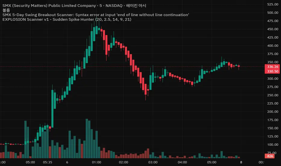
ICT Key Levels: PDH / PDL / Daily Open//@version=5
indicator("ICT Key Levels: PDH / PDL / Daily Open", shorttitle="ICT Levels", overlay=true)
// --- Inputs
showPD = input.bool(true, "Mostrar PDH/PDL")
showOpen = input.bool(true, "Mostrar Daily Open")
pdhColor = input.color(color.new(color.green, 0), "Color PDH")
pdlColor = input.color(color.new(color.red, 0), "Color PDL")
openColor = input.color(color.new(color.orange, 0), "Color Daily Open")
lineWidth = input.int(1, "Ancho líneas", minval=1, maxval=4)
// --- Previous day high / low (using daily security)
pdh = request.security(syminfo.tickerid, "D", high )
pdl = request.security(syminfo.tickerid, "D", low )
// --- Daily open (current day's open on Daily timeframe)
dailyOpen = request.security(syminfo.tickerid, "D", open)
// --- Plots
plot(showPD and not na(pdh) ? pdh : na, title="PDH", color=pdhColor, linewidth=lineWidth, style=plot.style_line)
plot(showPD and not na(pdl) ? pdl : na, title="PDL", color=pdlColor, linewidth=lineWidth, style=plot.style_line)
plot(showOpen and not na(dailyOpen) ? dailyOpen : na, title="Daily Open", color=openColor, linewidth=lineWidth, style=plot.style_line)
// --- Optional: etiquetas en inicio de día (solo en la primera barra diaria)
isNewDay = ta.change(time("D"))
labelNewDayOpen = input.bool(true, "Mostrar etiqueta en apertura diaria")
if labelNewDayOpen and isNewDay
label.new(bar_index, dailyOpen, text="Open", style=label.style_label_down, color=color.new(openColor,50), textcolor=color.black, yloc=yloc.price)

My script//@version=5
indicator("LTF Multi-Condition BUY Signal (v5 clean)", overlay=true, max_labels_count=100, max_lines_count=100)
// ───────────────── INPUTS ─────────────────
pivot_len = input.int(4, "Pivot sensitivity (structure)", minval=2, maxval=12)
range_len = input.int(20, "Range lookback for breakout", minval=5)
htf_tf = input.timeframe("480", "HTF timeframe (8H+)")
reclaim_window = input.int(5, "Reclaim window (bars)", minval=1)
ema_fast_len = input.int(9, "EMA fast length")
ema_slow_len = input.int(21, "EMA slow length")
rsi_len = input.int(14, "RSI length")
rsi_pivot_len = input.int(4, "RSI pivot sensitivity")
rsi_div_lookback = input.int(30, "RSI divergence max lookback (bars)")
daily_vol_mult = input.float(1.0, "Daily volume vs SMA multiplier", step=0.1)
htf_vol_sma_len = input.int(20, "HTF volume SMA length")
require_reclaim = input.bool(true, "Require HTF reclaim")
use_aggressive_HL = input.bool(false, "Aggressive HL detection")
// ───────────────── BASE INDICATORS ─────────────────
emaFast = ta.ema(close, ema_fast_len)
emaSlow = ta.ema(close, ema_slow_len)
rsiVal = ta.rsi(close, rsi_len)
// ───────────────── DAILY CHECKS (VOLUME & OBV) ─────────────────
// Daily OBV and previous value
daily_obv = request.security(syminfo.tickerid, "D",
ta.cum(ta.change(close) > 0 ? volume : ta.change(close) < 0 ? -volume : 0))
daily_obv_prev = request.security(syminfo.tickerid, "D",
ta.cum(ta.change(close) > 0 ? volume : ta.change(close) < 0 ? -volume : 0) )
// Daily volume & SMA
daily_vol = request.security(syminfo.tickerid, "D", volume)
daily_vol_sma = request.security(syminfo.tickerid, "D", ta.sma(volume, 20))
daily_vol_ok = not na(daily_vol) and not na(daily_vol_sma) and daily_vol > daily_vol_sma * daily_vol_mult
daily_obv_ok = not na(daily_obv) and not na(daily_obv_prev) and daily_obv > daily_obv_prev
// ───────────────── HTF SUPPORT / RECLAIM ─────────────────
htf_high = request.security(syminfo.tickerid, htf_tf, high)
htf_low = request.security(syminfo.tickerid, htf_tf, low)
htf_close = request.security(syminfo.tickerid, htf_tf, close)
htf_volume = request.security(syminfo.tickerid, htf_tf, volume)
htf_vol_sma = request.security(syminfo.tickerid, htf_tf, ta.sma(volume, htf_vol_sma_len))
htf_bull_reject = not na(htf_high) and not na(htf_low) and not na(htf_close) and (htf_close - htf_low) > (htf_high - htf_close)
htf_vol_confirm = not na(htf_volume) and not na(htf_vol_sma) and htf_volume > htf_vol_sma
htf_support_level = (htf_bull_reject and htf_vol_confirm) ? htf_low : na
// Reclaim: LTF close back above HTF support within N bars
reclaimed_now = not na(htf_support_level) and close > htf_support_level and ta.barssince(close <= htf_support_level) <= reclaim_window
htf_reclaim_ok = require_reclaim ? reclaimed_now : true
// ───────────────── STRUCTURE: BOS & HL (CoC) ─────────────────
swingHighVal = ta.pivothigh(high, pivot_len, pivot_len)
swingLowVal = ta.pivotlow(low, pivot_len, pivot_len)
swingHighCond = not na(swingHighVal)
swingLowCond = not na(swingLowVal)
lastSwingHigh = ta.valuewhen(swingHighCond, swingHighVal, 0)
prevSwingHigh = ta.valuewhen(swingHighCond, swingHighVal, 1)
lastSwingLow = ta.valuewhen(swingLowCond, swingLowVal, 0)
prevSwingLow = ta.valuewhen(swingLowCond, swingLowVal, 1)
bos_bull = not na(prevSwingHigh) and close > prevSwingHigh
hl_confirm = not na(lastSwingLow) and not na(prevSwingLow) and lastSwingLow > prevSwingLow and ta.barssince(swingLowCond) <= 30
if use_aggressive_HL
hl_confirm := hl_confirm or (low > low and ta.barssince(swingLowCond) <= 12)
// ───────────────── RSI BULLISH DIVERGENCE ─────────────────
rsiLowVal = ta.pivotlow(rsiVal, rsi_pivot_len, rsi_pivot_len)
rsiLowCond = not na(rsiLowVal)
priceAtRsiLowA = ta.valuewhen(rsiLowCond, low , 0)
priceAtRsiLowB = ta.valuewhen(rsiLowCond, low , 1)
rsiLowA = ta.valuewhen(rsiLowCond, rsiVal , 0)
rsiLowB = ta.valuewhen(rsiLowCond, rsiVal , 1)
rsi_div_ok = not na(priceAtRsiLowA) and not na(priceAtRsiLowB) and not na(rsiLowA) and not na(rsiLowB) and
(priceAtRsiLowA < priceAtRsiLowB) and (rsiLowA > rsiLowB) and ta.barssince(rsiLowCond) <= rsi_div_lookback
// ───────────────── RANGE BREAKOUT ─────────────────
range_high = ta.highest(high, range_len)
range_breakout = ta.crossover(close, range_high)
// ───────────────── EMA CROSS / TREND ─────────────────
ema_cross_happened = ta.crossover(emaFast, emaSlow)
ema_trend_ok = emaFast > emaSlow
// ───────────────── FINAL BUY CONDITION ─────────────────
all_price_checks = bos_bull and hl_confirm and rsi_div_ok and range_breakout
all_filter_checks = ema_trend_ok and ema_cross_happened and daily_vol_ok and daily_obv_ok and htf_reclaim_ok
buy_condition = all_price_checks and all_filter_checks
// ───────────────── PLOTS & ALERT ─────────────────
plotshape(
buy_condition,
title = "BUY Signal",
location = location.belowbar,
style = shape.labelup,
text = "BUY",
textcolor = color.white,
color = color.green,
size = size.small)
plot(htf_support_level, title="HTF Support", color=color.new(color.green, 0), linewidth=2, style=plot.style_linebr)
alertcondition(buy_condition, title="LTF BUY Signal", message="LTF BUY Signal on {{ticker}} ({{interval}}) — all conditions met")

Vol-Pace Projected-ATR-ADX-Alert-MAThe VolSC indicator analyzes stock volume trends with a focus on the Pace metric, which projects today's volume as a percentage of the 30-day average, highlighting unusual activity (e.g., over 200% turns bright green with alerts). The phantom projection bar, a wide green histogram to the right of the last bar, visually represents this projected volume on daily charts only, aiding quick identification of potential volume surges without cluttering intraday or weekly views. Additional features include ADX strength, ATR averages, and customizable table display for comprehensive insights.
Key Features:
* Primary Indicator: Volume with ADX (Average Directional Index) text.
* Pacing and Alerts: Calculates the volume pace for the day. Features an unusual volume alert with an adjustable threshold (e.g., 200%).
* Volume Projection: Projects a visual "Phantom Volume" for the day, offset to the right of the actual volume bar.
* ATR Indicator: Displays the 2x ATR (Average True Range) value as text.
* Volume Average: Displays the ADV (Average Daily Volume) Moving Average as text.
* Customization: Most settings are adjustable.
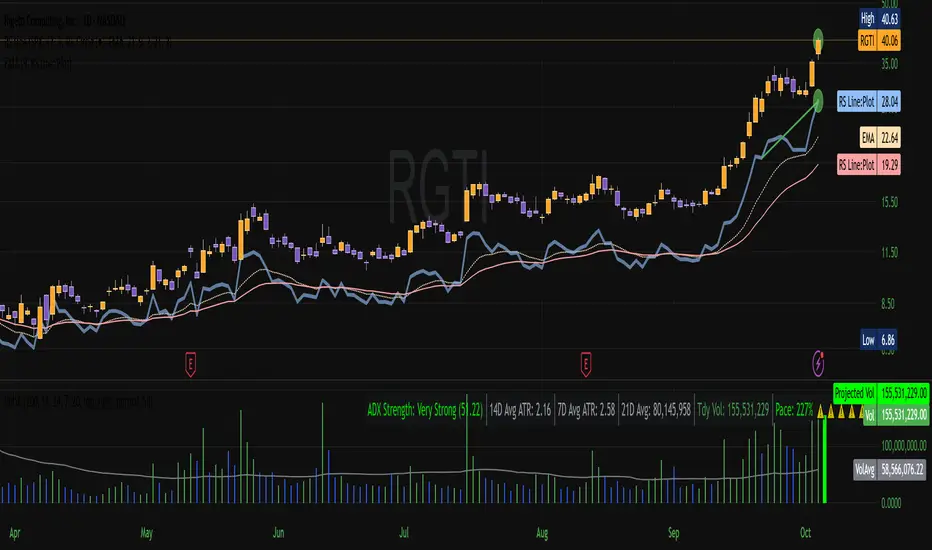
Stoch + RSI DashboardIndicator Description
MTF Stochastic + RSI Dashboard FLEX with STRONG Alerts
A compact, multi-timeframe dashboard that shows Stochastic %K/%D, RSI and signal states across user-defined timeframes. Columns can be toggled on/off to keep the panel as small as you need. Signal texts and colors are fully customizable. The table can be placed in any chart corner, and the background color & opacity are adjustable for perfect readability.
What it shows
• For each selected timeframe: %K, %D, a signal cell (Bullish/Bearish/Strong), RSI value, and RSI state (Overbought/Oversold/Neutral).
• Timeframes are displayed as friendly labels (e.g., 60 → 1h, W → 1w, 3D → 3d).
Signals & logic
• Bullish/Bearish when %K and %D show a sufficient gap (or an optional confirmed cross).
• Strong Bullish when both %K and %D are below the “Strong Bullish max” threshold.
• Strong Bearish when both %K and %D are above the “Strong Bearish min” threshold.
• Optional confirmation: RSI < 30 for Strong Bullish, RSI > 70 for Strong Bearish.
Alerts
• Global alerts for any selected timeframes when a STRONG BULLISH or STRONG BEARISH event occurs.
Key options
• Column visibility toggles (TF, %K, %D, Signal, RSI, RSI Status).
• Custom signal texts & colors.
• Dashboard position: top-left / top-right / bottom-left / bottom-right.
• Table background color + opacity (0 = opaque, 100 = fully transparent).
• Sensitivity (minimum %K–%D gap) and optional “cross-only” mode.
• Customizable timeframes for display and for alerts.
Default settings
• Stochastic: K=5, D=3, SmoothK=3
• RSI length: 14
• Decimals: 1
• Strong Bullish max: 20
• Strong Bearish min: 80
• Default TFs & alerts: 3m, 15m, 1h, 3h, 6h, 12h, 1d, 3d, 1w
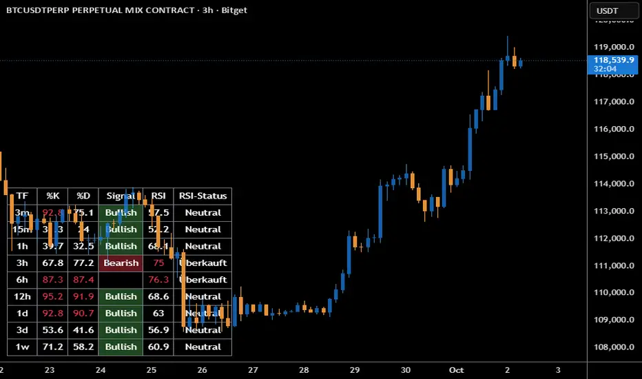
Volume Spike Alert & Overlay"Volume Spike Alert & Overlay" highlights unusually high trading volume on a chart. It calculates whether the current volume exceeds a user-defined percentage above the historical average and triggers an alert if it does. The information is also displayed in a customizable on-screen table.
What It Does
Monitors volume for each bar and compares it to an average over a user-defined lookback period.
Supports multiple smoothing methods (SMA, EMA, WMA, RMA) for calculating the average volume.
Triggers an alert when current volume exceeds the threshold percentage above the average.
Displays a table on the chart with:
Current Volume
Average Volume
Threshold Percentage
Optional empty row for spacing/formatting
How It Works
User Inputs:
lookbackPeriods: Number of bars used to calculate the average volume.
thresholdPercent: % above the average that triggers a volume spike alert.
smoothingType: Type of moving average used for volume calculation.
textColor, bgColor: Formatting for the display table.
tablePositionInput: Where the table appears on the chart (e.g., Bottom Right).
Toggles for showing/hiding parts of the table.
Volume Calculations:
Calculates current bar's volume.
Calculates average volume using the selected smoothing method.
Computes the threshold: avgVol * (1 + thresholdPercent / 100).
Compares current volume to threshold.
Table Display:
Dynamically creates a table with volume stats.
Adds rows based on user preferences.
Alerts:
alertcondition fires when currentVol crosses above the calculated threshold.
Message: "Volume Threshold Exceeded"
Usage Examples
Example 1: Spotting High Activity
Apply the script to a stock like AAPL on a 5-minute chart.
Set lookbackPeriods to 20 and thresholdPercent to 30.
Use EMA for more reactive volume tracking.
When volume spikes more than 30% above the 20-period EMA, an alert triggers.
Example 2: Day Trading Filter
For scalpers, apply it to a 1-minute crypto chart (e.g., BTC/USDT).
Set thresholdPercent to 50 to catch only strong surges.
Position the table at the top left and reduce visible info for a clean layout.
Example 3: Long-Term Context
On a daily chart, use SMA and set lookbackPeriods to 50.
Helps identify breakout moves supported by strong volume.
How this is different from Trading View's Volume indicator:
The standard volume plot from trading view allows users to set a alert when the average line is crossed, but it does not allow you to set a custom percentage at which to trigger an alert. This indicator will allow you to set any percentage you wish to monitor and above that percentage threshold will trigger your alert.
===== ORIGINAL DESCRIPTION =====
Volume Spike Alert & Overlay
This indicator will display the following as an overlay on your chart:
Current volume
Average Volume
Threshold for Alert
Description:
This indicator will display the current bar volume based on the chart time frame,
display the average volume based on selected conditions,
allow user selectable threshold over the average volume to trigger an alert.
Options:
Average lookback period
Smoothing type
Alert Threshold %
Enable / Disable Each Value
Change Text Color
Change Background Color
Change Table location
Add/Remove extra row for placement in top corner
Usage Example:
I use this indicator to alert when the current volume exceeds the average volume by a specified percentage to alert to volume spikes.
Set the threshold to 25% in the settings
Create an alert by clicking on the 3 dots on the right of the indicator title on the chart
When the threshold is exceeded the alert will trigger
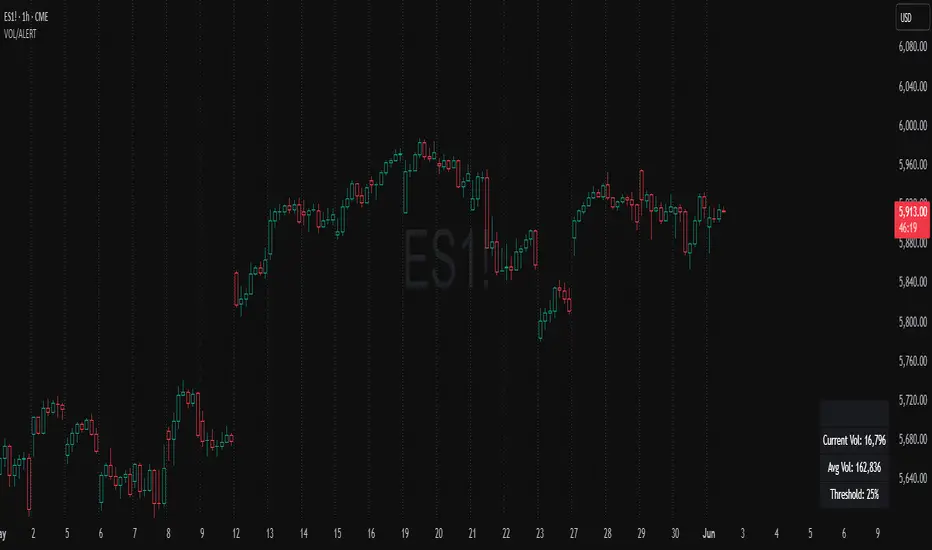
Intrabar DistributionThe Intrabar Distribution publication is an extension of the Intrabar BoxPlot publication. Besides a boxplot, it showcases price and volume distribution using intrabar Lower Timeframe (LTF) values (close) which can be displayed on the chart or in a separate pane.
🔶 USAGE
Intrabar Distribution has several features, users can display:
Recent candle for comparison against the other features
Boxplot of recent candle
Price distribution (optionally displayed as a curve)
Volume distribution
🔹 Recent candle / Boxplot
The middle 50% intrabar close values (Interquartile range, or IQR) are shown as a box, where the upper limit is percentile 75 (p75), and the lower limit is percentile 25 (p25). The dashed lines show the addition/subtraction of 1.5*IQR. All values out of range are considered outliers. They are displayed as white dots within the IQR*1.5 range or white X's when beyond the IQR*3 range (extreme outliers).
By showing the middle 50% intrabar values through a box, we can more easily see where the intrabar activity is mainly situated.
Note in the example above an upward-directed candle with a negative volume delta, displayed as a red box and dot (see further).
As seen in the following example, compared against the recent candle (grey candle at the left), most of the intrabar activity lies just beneath the opening price.
Note that results will be more accurate when more data is available, which can be done by making the difference between the current timeframe and the intrabar timeframe large enough.
🔹 Price / Volume distribution
The price and volume distribution can be helpful for highlighting areas of interest.
Here, we can see two areas where intrabar closing prices are mainly positioned.
The following example shows three successive bars. The recent bar is displayed on the left side, together with the volume distribution. The boxplot and price distribution are displayed on the right.
You can see the difference between volume and price distribution.
At the first bar, most price activity is at the top, while most of the volume was generated at the bottom; in other words, the price got briefly in the bottom region, with high volume before it returned.
At the second bar, price and volume are relatively equally distributed, which fits for indecisiveness.
The third bar shows more volume at a higher region; most intrabar closing prices are above the closing price.
Following example shows the same with 'Curve shaped' enabled (Settings: 'Price Distribution')
When 'Curve shaped' is enabled, lines/labels are shown with the standard deviation distance.
A blue 'guide line' can be enabled for easier interpretation.
🔹 Volume Delta
When there is a discrepancy between the delta volume and direction of the candle, this will be displayed as follows:
Red candle: when the sum of the volume of green intrabars is higher than the sum of the volume of red intrabars, the 'mean dot' will be coloured green.
Green candle: when the sum of the volume of red intrabars is higher than the sum of the volume of green intrabars, the 'mean dot' will be coloured red.
🔶 DETAILS
The intrabar values are sorted and split in parts/sections. The number of values in each section is displayed as a white line
The same principle applies to volume distribution, where the sum of volume per section is displayed as an orange area.
The boxplot displays several price values
Last close price
Highest / lowest intrabar close price
Median
p25 / p75
🔹 LTF settings
When 'Auto' is enabled (Settings, LTF), the LTF will be the nearest possible x times smaller TF than the current TF. When 'Premium' is disabled, the minimum TF will always be 1 minute to ensure TradingView plans lower than Premium don't get an error.
Examples with current Daily TF (when Premium is enabled):
500 : 3 minute LTF
1500 (default): 1 minute LTF
5000: 30 seconds LTF (1 minute if Premium is disabled)
🔶 SETTINGS
Location: Chart / Pane (when pane is opted, move the indicator to a separate pane as well)
Parts: divides the intrabar close values into parts/sections
Offset: offsets every drawing at once
Width: width of drawings, only applicable on "location: chart"
Label size: size of price labels
🔹 LTF
LTF: LTF setting
Auto + multiple: Adjusts the initial set LTF
Premium: Enable when your TradingView plan is Premium or higher
🔹 Current Bar
Display toggle + color setting
Offset: offsets only the 'Current Bar' drawing
🔹 Intrabar Boxplot
Display toggle + Colors, dependable on different circumstances.
Up: Price goes up, with more bullish than bearish intrabar volume.
Up-: Price goes up, with more bearish than bullish intrabar volume.
Down: Price goes down, with more bearish than bullish intrabar volume.
Down+: Price goes down, with more bullish than bearish intrabar volume.
Offset: offsets only the 'Boxplot' drawing
🔹 Price distribution
Display toggle + Color.
Curve Shaped
Guide Lines: Display 2 blue lines
Display Price: Show price of 'x' standard deviation
Offset: offsets only the 'Price distribution' drawing
Label size: size of price labels (standard deviation)
🔹 Volume distribution
Display toggle + Color.
Offset: offsets only the 'Volume distribution' drawing
🔹 Table
Show TF: Show intrabar Timeframe.
Textcolor
Size Table: Text Size
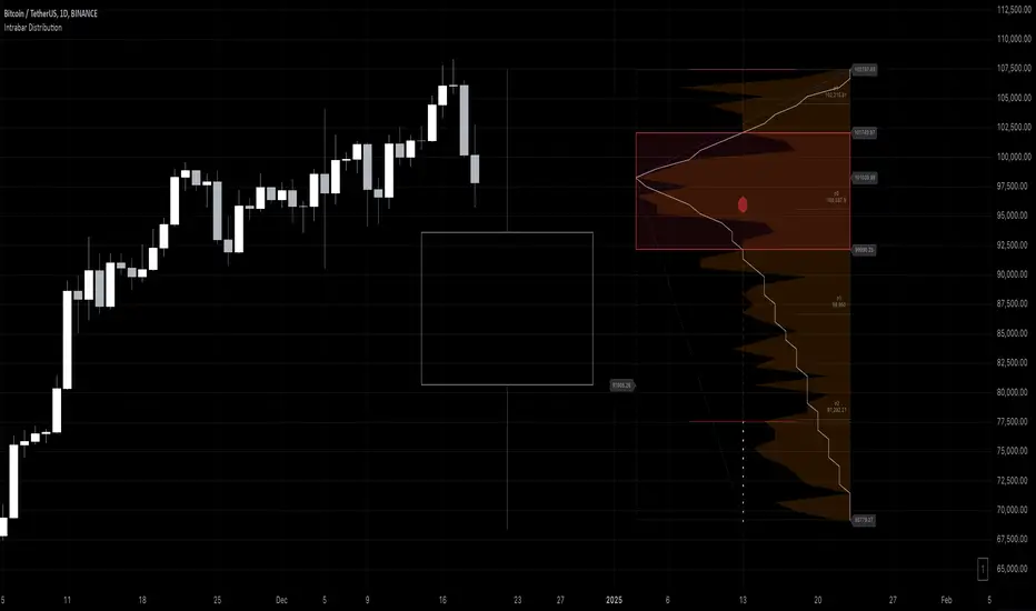
nPOC Levels by Tyler### Explanation of the Pine Script
This Pine Script identifies and displays weekly naked Points of Control (nPOCs) on a TradingView chart. An nPOC represents a Point of Control (POC) from a previous week that has not been revisited by price action in subsequent weeks. These nPOCs are extended to the right as horizontal lines, indicating potential support or resistance levels.
#### Script Overview
1. **Indicator Declaration:**
```pinescript
//@version=5
indicator("Weekly nPOCs", overlay=true)
```
- The script is defined as a version 5 Pine Script.
- The `indicator` function sets the script's name ("Weekly nPOCs") and specifies that the indicator should be overlaid on the price chart (`overlay=true`).
2. **Function to Calculate POC:**
```pinescript
f_poc(_hl2, _vol) =>
var float vol_profile = na
if (na(vol_profile))
vol_profile := array.new_float(100, 0.0)
_bin_size = (high - low) / 100
for i = 0 to 99
if _hl2 >= low + i * _bin_size and _hl2 < low + (i + 1) * _bin_size
array.set(vol_profile, i, array.get(vol_profile, i) + _vol)
max_volume = array.max(vol_profile)
poc_index = array.indexof(vol_profile, max_volume)
poc_price = low + poc_index * _bin_size + _bin_size / 2
poc_price
```
- The function `f_poc` calculates the Point of Control (POC) for a given period.
- It takes two parameters: `_hl2` (the average of the high and low prices) and `_vol` (volume).
- A volume profile array (`vol_profile`) is initialized to store volume data across different price bins.
- The price range between the high and low is divided into 100 bins (`_bin_size`).
- The function iterates over each bin, accumulating the volumes for prices within each bin.
- The bin with the maximum volume is identified as the POC (`poc_price`).
3. **Variables to Store Weekly Data:**
```pinescript
var float poc = na
var float prev_poc = na
var line poc_lines = na
if na(poc_lines)
poc_lines := array.new_line(0)
```
- `poc` stores the current week's POC.
- `prev_poc` stores the previous week's POC.
- `poc_lines` is an array to store lines representing nPOCs. The array is initialized if it is `na` (not initialized).
4. **Calculate Weekly POC:**
```pinescript
is_new_week = ta.change(time('W')) != 0
if (is_new_week)
prev_poc := poc
poc := f_poc(hl2, volume)
if not na(prev_poc)
line new_poc_line = line.new(x1=bar_index, y1=prev_poc, x2=bar_index + 100, y2=prev_poc, color=color.red, width=2)
label.new(x=bar_index, y=prev_poc, text="nPOC", style=label.style_label_down, color=color.red, textcolor=color.white)
array.push(poc_lines, new_poc_line)
```
- `is_new_week` checks if the current bar is the start of a new week using the `ta.change(time('W'))` function.
- If it's a new week, the previous week's POC is stored in `prev_poc`, and the current week's POC is calculated using `f_poc`.
- If `prev_poc` is not `na`, a new line (`new_poc_line`) representing the nPOC is created, extending it to the right (for 100 bars).
- A label is created at the `prev_poc` level, marking it as "nPOC".
- The new line is added to the `poc_lines` array.
5. **Remove Old Lines:**
```pinescript
if array.size(poc_lines) > 52
line.delete(array.shift(poc_lines))
```
- This section ensures that only the last 52 weeks of nPOCs are kept to avoid cluttering the chart.
- If the `poc_lines` array contains more than 52 lines, the oldest line is deleted using `array.shift`.
6. **Plot the Current Week's POC as a Reference:**
```pinescript
plot(poc, title="Current Weekly POC", color=color.blue, linewidth=2, style=plot.style_line)
```
- The current week's POC is plotted as a blue line on the chart for reference.
#### Summary
This script calculates and identifies weekly Points of Control (POCs) and marks them as nPOCs if they remain untouched by subsequent price action. These nPOCs are displayed as horizontal lines extending to the right, providing traders with potential support or resistance levels. The script also manages the number of lines plotted to maintain a clear and uncluttered chart.