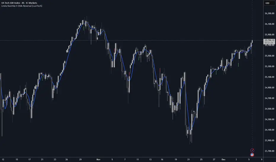
Linda Raschke 5 SMA Reversal [LuciTech]How This Indicator Works:
-5 SMA Tracking: Calculates a 5-period simple moving average and plots it on the chart.
-Extension Counter: Counts consecutive bars where price closes above or below the 5 SMA.
-BUY Signals (Green Up Arrow): Triggers when price closes BELOW the 5 SMA after 7+ consecutive closes ABOVE it—indicates a reversal opportunity into dynamic support.
-SELL Signals (Red Down Arrow): Triggers when price closes ABOVE the 5 SMA after 7+ consecutive closes BELOW it—indicates a reversal bounce setup.
-No Repainting: Signals only plot on confirmed bar closes; no repainting issues.
Linda Raschke's Core Principles:
-Extended Run = Imbalance: When price stays above/below the 5 SMA for 7+ bars, it's a one-sided market; mean reversion is likely.
-First Cross = Trigger: The first close back across the SMA after an extension is the reversal signal, not every touch.
-No Setup? No Trade: Without a prior extension or "three-bar balance" filter, a 5 SMA tag is noise. The model requires the prior momentum condition.
-Uptrend Buys: In uptrends, buy dips to the SMA (dynamic support) as long as the weekly/monthly trend is intact.
-Downtrend Fades: In downtrends, treat first rallies above the SMA as bounce fades into lower lows (especially after 14+ bars below).
在脚本中搜索"trigger"
Major exchages total Open interest & Long/Short OI trends📊 Indicator: Major Exchanges Total OI & Long/Short Trends
This Pine Script™ indicator is designed to provide a comprehensive analysis of Open Interest (OI) and Long/Short position trends across major cryptocurrency exchanges (Binance, Bybit, OKX, Bitget, HTX, Deribit). It serves as a powerful tool for traders seeking to understand market liquidity, participant positioning, and overall market sentiment.
🔑 Key Features and Functionalities
Aggregated Multi-Exchange Open Interest (OI):
Consolidates real-time Open Interest data from user-selected major cryptocurrency exchanges.
Provides a unified view of the total OI, offering insights into the collective market liquidity and the aggregate size of participants' open positions.
Visualized Combined OI Candles:
Presents the aggregated total OI data in a candlestick chart format.
Displays the Open, High, Low, and Close of the combined OI, with color variations indicating increases or decreases from the previous period. This enables intuitive visualization of OI trend shifts.
Estimated Long/Short OI and Visualization:
Calculates and visualizes estimated Long and Short position Open Interest based on the total aggregated OI data.
Estimation Logic:
Employs a sophisticated logic that considers both price changes and OI fluctuations to infer the balance between Long and Short positions. For instance, an increase in both price and OI may suggest an accumulation of Long positions, while a price decrease coupled with an OI increase might indicate growing Short positions.
Initial 50:50 Ratio:
The estimation for Long/Short OI begins with an assumption of a 50:50 ratio at the initial data point available for the selected timeframe. This establishes a neutral baseline, from which subsequent price and OI changes drive the divergence and evolution of the estimated Long/Short balance.
Flexible Visualization Options:
Allows users to display Long/Short OI data in either line or candlestick styles, with customizable color schemes. This flexibility aids in clearly discerning bullish or bearish positioning trends.
💡 Development Background
The development of this indicator stems from the critical importance of Open Interest data in the cryptocurrency derivatives market. Recognizing the limitations of analyzing individual exchange OI in isolation, the primary objective was to integrate data from leading exchanges to offer a holistic perspective on market sentiment and overall positioning dynamics.
The inclusion of the Long/Short position estimation feature is crucial for deciphering the specific directional biases of market participants, which is often not evident from raw OI data alone. This enables a deeper understanding of how positions are being accumulated or liquidated, moving beyond simple OI change analysis.
Furthermore, a key design consideration was to leverage the characteristic where the indicator's data start point dynamically adjusts with the chart's timeframe selection. This allows for the analysis of short-term Long/Short trends on shorter timeframes and long-term trends on longer timeframes. This inherent flexibility empowers traders to conduct analyses across various time scales, aligning with their diverse trading strategies.
🚀 Trading Applications
Leveraging Combined Open Interest (OI):
Trend Confirmation: A sustained increase in total OI signifies growing market interest and capital inflow, potentially confirming the strength of an existing trend. Conversely, decreasing OI may suggest diminishing participant interest or widespread position liquidation.
Validation of Price Extremes: If price forms a new high but OI fails to increase or declines, it could signal a potential trend reversal (divergence). Conversely, a sharp increase in OI during a price decline might indicate a surge in short positions or renewed selling pressure.
Identifying Volatility Triggers: Monitoring rapid shifts in OI during significant news events or market catalysts can help assess immediate market reactions and liquidity changes.
📈Utilizing Long/Short OI Trends
Assessing Market Bias: A sustained dominance or rapid increase in Long OI suggests a prevalent bullish sentiment, which could inform decisions to enter or maintain long positions. The inverse scenario indicates bearish sentiment and potential short entry opportunities.
Anticipating Squeezes: The indicator can help identify scenarios conducive to short or long squeezes. Excessive short positioning followed by a price uptick can trigger a short squeeze, leading to rapid price appreciation. Conversely, an oversupply of long positions preceding a price drop can result in a long squeeze and sharp declines.
Divergence Analysis: Divergences between price action and Long/Short OI estimates can signal potential trend reversals. For example, if price is rising but the increase in Long OI slows down or Short OI begins to grow, it may suggest weakening buying pressure.
🕔Timeframe-Specific Trend Analysis:
Shorter Timeframes (e.g., 1m, 5m, 15m): Ideal for identifying short-term shifts in participant positioning, beneficial for day trading and scalping strategies. Provides insights into immediate market reactions to price movements.
Longer Timeframes (e.g., 1h, 4h, Daily): Valuable for evaluating broader positioning trends and the sustainability or potential reversal of medium-to-long-term trends. Offers a macro perspective on Long/Short dynamics, suitable for swing trading or long-term investment strategies.
This indicator integrates complex market data, provides nuanced Long/Short position estimations, and offers multi-timeframe analytical capabilities, empowering traders to make more informed and strategic decisions.

COT IndexTHE HIDDEN INTELLIGENCE IN FUTURES MARKETS
What if you could see what the smartest players in the futures markets are doing before the crowd catches on? While retail traders chase momentum indicators and moving averages, obsess over Japanese candlestick patterns, and debate whether the RSI should be set to fourteen or twenty-one periods, institutional players leave footprints in the sand through their mandatory reporting to the Commodity Futures Trading Commission. These footprints, published weekly in the Commitment of Traders reports, have been hiding in plain sight for decades, available to anyone with an internet connection, yet remarkably few traders understand how to interpret them correctly. The COT Index indicator transforms this raw institutional positioning data into actionable trading signals, bringing Wall Street intelligence to your trading screen without requiring expensive Bloomberg terminals or insider connections.
The uncomfortable truth is this: Most retail traders operate in a binary world. Long or short. Buy or sell. They apply technical analysis to individual positions, constrained by limited capital that forces them to concentrate risk in single directional bets. Meanwhile, institutional traders operate in an entirely different dimension. They manage portfolios dynamically weighted across multiple markets, adjusting exposure based on evolving market conditions, correlation shifts, and risk assessments that retail traders never see. A hedge fund might be simultaneously long gold, short oil, neutral on copper, and overweight agricultural commodities, with position sizes calibrated to volatility and portfolio Greeks. When they increase gold exposure from five percent to eight percent of portfolio allocation, this rebalancing decision reflects sophisticated analysis of opportunity cost, risk parity, and cross-market dynamics that no individual chart pattern can capture.
This portfolio reweighting activity, multiplied across hundreds of institutional participants, manifests in the aggregate positioning data published weekly by the CFTC. The Commitment of Traders report does not show individual trades or strategies. It shows the collective footprint of how actual commercial hedgers and large speculators have allocated their capital across different markets. When mining companies collectively increase forward gold sales to hedge thirty percent more production than last quarter, they are not reacting to a moving average crossover. They are making strategic allocation decisions based on production forecasts, cost structures, and price expectations derived from operational realities invisible to outside observers. This is portfolio management in action, revealed through positioning data rather than price charts.
If you want to understand how institutional capital actually flows, how sophisticated traders genuinely position themselves across market cycles, the COT report provides a rare window into that hidden world. But understand what you are getting into. This is not a tool for scalpers seeking confirmation of the next five-minute move. This is not an oscillator that flashes oversold at market bottoms with convenient precision. COT analysis operates on a timescale measured in weeks and months, revealing positioning shifts that precede major market turns but offer no precision timing. The data arrives three days stale, published only once per week, capturing strategic positioning rather than tactical entries.
If you need instant gratification, if you trade intraday moves, if you demand mechanical signals with ninety percent accuracy, close this document now. COT analysis rewards patience, position sizing discipline, and tolerance for being early. It punishes impatience, overleveraging, and the expectation that any single indicator can substitute for market understanding.
The premise is deceptively simple. Every Tuesday, large traders in futures markets must report their positions to the CFTC. By Friday afternoon, this data becomes public. Academic research spanning three decades has consistently shown that not all market participants are created equal. Some traders consistently profit while others consistently lose. Some anticipate major turning points while others chase trends into exhaustion. Bessembinder and Chan (1992) demonstrated in their seminal study that commercial hedgers, those with actual exposure to the underlying commodity or financial instrument, possess superior forecasting ability compared to speculators. Their research, published in the Journal of Finance, found statistically significant predictive power in commercial positioning, particularly at extreme levels. This finding challenged the efficient market hypothesis and opened the door to a new approach to market analysis based on positioning rather than price alone.
Think about what this means. Every week, the government publishes a report showing you exactly how the most informed market participants are positioned. Not their opinions. Not their predictions. Their actual money at risk. When agricultural producers collectively hold their largest short hedge in five years, they are not making idle speculation. They are locking in prices for crops they will harvest, informed by private knowledge of weather conditions, soil quality, inventory levels, and demand expectations invisible to outside observers. When energy companies aggressively hedge forward production at current prices, they reveal information about expected supply that no analyst report can capture. This is not technical analysis based on past prices. This is not fundamental analysis based on publicly available data. This is behavioral analysis based on how the smartest money is actually positioned, how institutions allocate capital across portfolios, and how those allocation decisions shift as market conditions evolve.
WHY SOME TRADERS KNOW MORE THAN OTHERS
Building on this foundation, Sanders, Boris and Manfredo (2004) conducted extensive research examining the behaviour patterns of different trader categories. Their work, which analyzed over a decade of COT data across multiple commodity markets, revealed a fascinating dynamic that challenges much of what retail traders are taught. Commercial hedgers consistently positioned themselves against market extremes, buying when speculators were most bearish and selling when speculators reached peak bullishness. The contrarian positioning of commercials was not random noise but rather reflected their superior information about supply and demand fundamentals. Meanwhile, large speculators, primarily hedge funds and commodity trading advisors, exhibited strong trend-following behaviour that often amplified market moves beyond fundamental values. Small traders, the retail participants, consistently entered positions late in trends, frequently near turning points, making them reliable contrary indicators.
Wang (2003) extended this research by demonstrating that the predictive power of commercial positioning varies significantly across different commodity sectors. His analysis of agricultural commodities showed particularly strong forecasting ability, with commercial net positions explaining up to fifteen percent of return variance in subsequent weeks. This finding suggests that the informational advantages of hedgers are most pronounced in markets where physical supply and demand fundamentals dominate, as opposed to purely financial markets where information asymmetries are smaller. When a corn farmer hedges six months of expected harvest, that decision incorporates private observations about rainfall patterns, crop health, pest pressure, and local storage capacity that no distant analyst can match. When an oil refinery hedges crude oil purchases and gasoline sales simultaneously, the spread relationships reveal expectations about refining margins that reflect operational realities invisible in public data.
The theoretical mechanism underlying these empirical patterns relates to information asymmetry and different participant motivations. Commercial hedgers engage in futures markets not for speculative profit but to manage business risks. An agricultural producer selling forward six months of expected harvest is not making a bet on price direction but rather locking in revenue to facilitate financial planning and ensure business viability. However, this hedging activity necessarily incorporates private information about expected supply, inventory levels, weather conditions, and demand trends that the hedger observes through their commercial operations (Irwin and Sanders, 2012). When aggregated across many participants, this private information manifests in collective positioning.
Consider a gold mining company deciding how much forward production to hedge. Management must estimate ore grades, recovery rates, production costs, equipment reliability, labor availability, and dozens of other operational variables that determine whether locking in prices at current levels makes business sense. If the industry collectively hedges more aggressively than usual, it suggests either exceptional production expectations or concern about sustaining current price levels or combination of both. Either way, this positioning reveals information unavailable to speculators analyzing price charts and economic data. The hedger sees the physical reality behind the financial abstraction.
Large speculators operate under entirely different incentives and constraints. Commodity Trading Advisors managing billions in assets typically employ systematic, trend-following strategies that respond to price momentum rather than fundamental supply and demand. When crude oil rallies from sixty dollars to seventy dollars per barrel, these systems generate buy signals. As the rally continues to eighty dollars, position sizes increase. The strategy works brilliantly during sustained trends but becomes a liability at reversals. By the time oil reaches ninety dollars, trend-following funds are maximally long, having accumulated positions progressively throughout the rally. At this point, they represent not smart money anticipating further gains but rather crowded money vulnerable to reversal. Sanders, Boris and Manfredo (2004) documented this pattern across multiple energy markets, showing that extreme speculator positioning typically marked late-stage trend exhaustion rather than early-stage trend development.
Small traders, the retail participants who fall below reporting thresholds, display the weakest forecasting ability. Wang (2003) found that small trader positioning exhibited negative correlation with subsequent returns, meaning their aggregate positioning served as a reliable contrary indicator. The explanation combines several factors. Retail traders often lack the capital reserves to weather normal market volatility, leading to premature exits from positions that would eventually prove profitable. They tend to receive information through slower channels, entering trends after mainstream media coverage when institutional participants are preparing to exit. Perhaps most importantly, they trade with emotion, buying into euphoria and selling into panic at precisely the wrong times.
At major turning points, the three groups often position opposite each other with commercials extremely bearish, large speculators extremely bullish, and small traders piling into longs at the last moment. These high-divergence environments frequently precede increased volatility and trend reversals. The insiders with business exposure quietly exit as the momentum traders hit maximum capacity and retail enthusiasm peaks. Within weeks, the reversal begins, and positions unwind in the opposite sequence.
FROM RAW DATA TO ACTIONABLE SIGNALS
The COT Index indicator operationalizes these academic findings into a practical trading tool accessible through TradingView. At its core, the indicator normalizes net positioning data onto a zero to one hundred scale, creating what we call the COT Index. This normalization is critical because absolute position sizes vary dramatically across different futures contracts and over time. A commercial trader holding fifty thousand contracts net long in crude oil might be extremely bullish by historical standards, or it might be quite neutral depending on the context of total market size and historical ranges. Raw position numbers mean nothing without context. The COT Index solves this problem by calculating where current positioning stands relative to its range over a specified lookback period, typically two hundred fifty-two weeks or approximately five years of weekly data.
The mathematical transformation follows the methodology originally popularized by legendary trader Larry Williams, though the underlying concept appears in statistical normalization techniques across many fields. For any given trader category, we calculate the highest and lowest net position values over the lookback period, establishing the historical range for that specific market and trader group. Current positioning is then expressed as a percentage of this range, where zero represents the most bearish positioning ever seen in the lookback window and one hundred represents the most bullish extreme. A reading of fifty indicates positioning exactly in the middle of the historical range, suggesting neither extreme optimism nor pessimism relative to recent history (Williams and Noseworthy, 2009).
This index-based approach allows for meaningful comparison across different markets and time periods, overcoming the scaling problems inherent in analyzing raw position data. A commercial index reading of eighty-five in gold carries the same interpretive meaning as an eighty-five reading in wheat or crude oil, even though the absolute position sizes differ by orders of magnitude. This standardization enables systematic analysis across entire futures portfolios rather than requiring market-specific expertise for each contract.
The lookback period selection involves a fundamental tradeoff between responsiveness and stability. Shorter lookback periods, perhaps one hundred twenty-six weeks or approximately two and a half years, make the index more sensitive to recent positioning changes. However, it also increases noise and produces more false signals. Longer lookback periods, perhaps five hundred weeks or approximately ten years, create smoother readings that filter short-term noise but become slower to recognize regime changes. The indicator settings allow users to adjust this parameter based on their trading timeframe, risk tolerance, and market characteristics.
UNDERSTANDING CFTC DATA STRUCTURES
The indicator supports both Legacy and Disaggregated COT report formats, reflecting the evolution of CFTC reporting standards over decades of market development. Legacy reports categorize market participants into three broad groups: commercial traders (hedgers with underlying business exposure), non-commercial traders (large speculators seeking profit without commercial interest), and non-reportable traders (small speculators below reporting thresholds). Each category brings distinct motivations and information advantages to the market (CFTC, 2020).
The Disaggregated reports, introduced in September 2009 for physical commodity markets, provide finer granularity by splitting participants into five categories (CFTC, 2009). Producer and merchant positions capture those actually producing, processing, or merchandising the physical commodity. Swap dealers represent financial intermediaries facilitating derivative transactions for clients. Managed money includes commodity trading advisors and hedge funds executing systematic or discretionary strategies. Other reportables encompasses diverse participants not fitting the main categories. Small traders remain as the fifth group, representing retail participation.
This enhanced categorization reveals nuances invisible in Legacy reports, particularly distinguishing between different types of institutional capital and their distinct behavioural patterns. The indicator automatically detects which report type is appropriate for each futures contract and adjusts the display accordingly.
Importantly, Disaggregated reports exist only for physical commodity futures. Agricultural commodities like corn, wheat, and soybeans have Disaggregated reports because clear producer, merchant, and swap dealer categories exist. Energy commodities like crude oil and natural gas similarly have well-defined commercial hedger categories. Metals including gold, silver, and copper also receive Disaggregated treatment (CFTC, 2009). However, financial futures such as equity index futures, Treasury bond futures, and currency futures remain available only in Legacy format. The CFTC has indicated no plans to extend Disaggregated reporting to financial futures due to different market structures and participant categories in these instruments (CFTC, 2020).
THE BEHAVIORAL FOUNDATION
Understanding which trader perspective to follow requires appreciation of their distinct trading styles, success rates, and psychological profiles. Commercial hedgers exhibit anticyclical behaviour rooted in their fundamental knowledge and business imperatives. When agricultural producers hedge forward sales during harvest season, they are not speculating on price direction but rather locking in revenue for crops they will harvest. Their business requires converting volatile commodity exposure into predictable cash flows to facilitate planning and ensure survival through difficult periods. Yet their aggregate positioning reveals valuable information because these hedging decisions incorporate private information about supply conditions, inventory levels, weather observations, and demand expectations that hedgers observe through their commercial operations (Bessembinder and Chan, 1992).
Consider a practical example from energy markets. Major oil companies continuously hedge portions of forward production based on price levels, operational costs, and financial planning needs. When crude oil trades at ninety dollars per barrel, they might aggressively hedge the next twelve months of production, locking in prices that provide comfortable profit margins above their extraction costs. This hedging appears as short positioning in COT reports. If oil rallies further to one hundred dollars, they hedge even more aggressively, viewing these prices as exceptional opportunities to secure revenue. Their short positioning grows increasingly extreme. To an outside observer watching only price charts, the rally suggests bullishness. But the commercial positioning reveals that the actual producers of oil find these prices attractive enough to lock in years of sales, suggesting skepticism about sustaining even higher levels. When the eventual reversal occurs and oil declines back to eighty dollars, the commercials who hedged at ninety and one hundred dollars profit while speculators who chased the rally suffer losses.
Large speculators or managed money traders operate under entirely different incentives and constraints. Their systematic, momentum-driven strategies mean they amplify existing trends rather than anticipate reversals. Trend-following systems, the most common approach among large speculators, by definition require confirmation of trend through price momentum before entering positions (Sanders, Boris and Manfredo, 2004). When crude oil rallies from sixty dollars to eighty dollars per barrel over several months, trend-following algorithms generate buy signals based on moving average crossovers, breakouts, and other momentum indicators. As the rally continues, position sizes increase according to the systematic rules.
However, this approach becomes a liability at turning points. By the time oil reaches ninety dollars after a sustained rally, trend-following funds are maximally long, having accumulated positions progressively throughout the move. At this point, their positioning does not predict continued strength. Rather, it often marks late-stage trend exhaustion. The psychological and mechanical explanation is straightforward. Trend followers by definition chase price momentum, entering positions after trends establish rather than anticipating them. Eventually, they become fully invested just as the trend nears completion, leaving no incremental buying power to sustain the rally. When the first signs of reversal appear, systematic stops trigger, creating a cascade of selling that accelerates the downturn.
Small traders consistently display the weakest track record across academic studies. Wang (2003) found that small trader positioning exhibited negative correlation with subsequent returns in his analysis across multiple commodity markets. This result means that whatever small traders collectively do, the opposite typically proves profitable. The explanation for small trader underperformance combines several factors documented in behavioral finance literature. Retail traders often lack the capital reserves to weather normal market volatility, leading to premature exits from positions that would eventually prove profitable. They tend to receive information through slower channels, learning about commodity trends through mainstream media coverage that arrives after institutional participants have already positioned. Perhaps most importantly, retail traders are more susceptible to emotional decision-making, buying into euphoria and selling into panic at precisely the wrong times (Tharp, 2008).
SETTINGS, THRESHOLDS, AND SIGNAL GENERATION
The practical implementation of the COT Index requires understanding several key features and settings that users can adjust to match their trading style, timeframe, and risk tolerance. The lookback period determines the time window for calculating historical ranges. The default setting of two hundred fifty-two bars represents approximately one year on daily charts or five years on weekly charts, balancing responsiveness with stability. Conservative traders seeking only the most extreme, highest-probability signals might extend the lookback to five hundred bars or more. Aggressive traders seeking earlier entry and willing to accept more false positives might reduce it to one hundred twenty-six bars or even less for shorter-term applications.
The bullish and bearish thresholds define signal generation levels. Default settings of eighty and twenty respectively reflect academic research suggesting meaningful information content at these extremes. Readings above eighty indicate positioning in the top quintile of the historical range, representing genuine extremes rather than temporary fluctuations. Conversely, readings below twenty occupy the bottom quintile, indicating unusually bearish positioning (Briese, 2008).
However, traders must recognize that appropriate thresholds vary by market, trader category, and personal risk tolerance. Some futures markets exhibit wider positioning swings than others due to seasonal patterns, volatility characteristics, or participant behavior. Conservative traders seeking high-probability setups with fewer signals might raise thresholds to eighty-five and fifteen. Aggressive traders willing to accept more false positives for earlier entry could lower them to seventy-five and twenty-five.
The key is maintaining meaningful differentiation between bullish, neutral, and bearish zones. The default settings of eighty and twenty create a clear three-zone structure. Readings from zero to twenty represent bearish territory where the selected trader group holds unusually bearish positions. Readings from twenty to eighty represent neutral territory where positioning falls within normal historical ranges. Readings from eighty to one hundred represent bullish territory where the selected trader group holds unusually bullish positions.
The trading perspective selection determines which participant group the indicator follows, fundamentally shaping interpretation and signal meaning. For counter-trend traders seeking reversal opportunities, monitoring commercial positioning makes intuitive sense based on the academic research discussed earlier. When commercials reach extreme bearish readings below twenty, indicating unprecedented short positioning relative to recent history, they are effectively betting against the crowd. Given their informational advantages demonstrated by Bessembinder and Chan (1992), this contrarian stance often precedes major bottoms.
Trend followers might instead monitor large speculator positioning, but with inverted logic compared to commercials. When managed money reaches extreme bullish readings above eighty, the trend may be exhausting rather than accelerating. This seeming paradox reflects their late-cycle participation documented by Sanders, Boris and Manfredo (2004). Sophisticated traders thus use speculator extremes as fade signals, entering positions opposite to speculator consensus.
Small trader monitoring serves primarily as a contrary indicator for all trading styles. Extreme small trader bullishness above seventy-five or eighty typically warns of retail FOMO at market tops. Extreme small trader bearishness below twenty or twenty-five often marks capitulation bottoms where the last weak hands have sold.
VISUALIZATION AND USER INTERFACE
The visual design incorporates multiple elements working together to facilitate decision-making and maintain situational awareness during active trading. The primary COT Index line plots in bold with adjustable line width, defaulting to two pixels for clear visibility against busy price charts. An optional glow effect, controlled by a simple toggle, adds additional visual prominence through multiple plot layers with progressively increasing transparency and width.
A twenty-one period exponential moving average overlays the index line, providing trend context for positioning changes. When the index crosses above its moving average, it signals accelerating bullish sentiment among the selected trader group regardless of whether absolute positioning is extreme. Conversely, when the index crosses below its moving average, it signals deteriorating sentiment and potentially the beginning of a reversal in positioning trends.
The EMA provides a dynamic reference line for assessing positioning momentum. When the index trades far above its EMA, positioning is not only extreme in absolute terms but also building with momentum. When the index trades far below its EMA, positioning is contracting or reversing, which may indicate weakening conviction even if absolute levels remain elevated.
The data table positioned at the top right of the chart displays eleven metrics for each trader category, transforming the indicator from a simple index calculation into an analytical dashboard providing multidimensional market intelligence. Beyond the COT Index itself, users can monitor positioning extremity, which measures how unusual current levels are compared to historical norms using statistical techniques. The extremity metric clarifies whether a reading represents the ninety-fifth or ninety-ninth percentile, with values above two standard deviations indicating genuinely exceptional positioning.
Market power quantifies each group's influence on total open interest. This metric expresses each trader category's net position as a percentage of total market open interest. A commercial entity holding forty percent of total open interest commands significantly more influence than one holding five percent, making their positioning signals more meaningful.
Momentum and rate of change metrics reveal whether positions are building or contracting, providing early warning of potential regime shifts. Position velocity measures the rate of change in positioning changes, effectively a second derivative providing even earlier insight into inflection points.
Sentiment divergence highlights disagreements between commercial and speculative positioning. This metric calculates the absolute difference between normalized commercial and large speculator index values. Wang (2003) found that these high-divergence environments frequently preceded increased volatility and reversals.
The table also displays concentration metrics when available, showing how positioning is distributed among the largest handful of traders in each category. High concentration indicates a few dominant players controlling most of the positioning, while low concentration suggests broad-based participation across many traders.
THE ALERT SYSTEM AND MONITORING
The alert system, comprising five distinct alert conditions, enables systematic monitoring of dozens of futures markets without constant screen watching. The bullish and bearish COT signal alerts trigger when the index crosses user-defined thresholds, indicating the selected trader group has reached extreme positioning worthy of attention. These alerts fire in real-time as new weekly COT data publishes, typically Friday afternoon following the Tuesday measurement date.
Extreme positioning alerts fire at ninety and ten index levels, representing the top and bottom ten percent of the historical range, warning of particularly stretched readings that historically precede reversals with high probability. When commercials reach a COT Index reading below ten, they are expressing their most bearish stance in the entire lookback period.
The data staleness alert notifies users when COT reports have not updated for more than ten days, preventing reliance on outdated information for trading decisions. Government shutdowns or federal holidays can interrupt the normal Friday publication schedule. Using stale signals while believing them current creates dangerous false confidence.
The indicator's watermark information display positioned in the bottom right corner provides essential context at a glance. This persistent display shows the symbol and timeframe, the COT report date timestamp, days since last update, and the current signal state. A trader analyzing a potential short entry in crude oil can glance at the watermark to instantly confirm positioning context without interrupting analysis flow.
LIMITATIONS AND REALISTIC EXPECTATIONS
Practical application requires understanding both the indicator's considerable strengths and inherent limitations. COT data inherently lags price action by three days, as Tuesday positions are not published until Friday afternoon. This delay means the indicator cannot catch rapid intraday reversals or respond to surprise news events. Traders using the COT Index for timing entries must accept this latency and focus on swing trading and position trading timeframes where three-day lags matter less than in day trading or scalping.
The weekly publication schedule similarly makes the indicator unsuitable for short-term trading strategies requiring immediate feedback. The COT Index works best for traders operating on weekly or longer timeframes, where positioning shifts measured in weeks and months align with trading horizon.
Extreme COT readings can persist far longer than typical technical indicators suggest, testing the patience and capital reserves of traders attempting to fade them. When crude oil enters a sustained bull market driven by genuine supply disruptions, commercial hedgers may maintain bearish positioning for many months as prices grind higher. A commercial COT Index reading of fifteen indicating extreme bearishness might persist for three months while prices continue rallying before finally reversing. Traders without sufficient capital and risk tolerance to weather such drawdowns will exit prematurely, precisely when the signal is about to work (Irwin and Sanders, 2012).
Position sizing discipline becomes paramount when implementing COT-based strategies. Rather than risking large percentages of capital on individual signals, successful COT traders typically allocate modest position sizes across multiple signals, allowing some to take time to mature while others work more quickly.
The indicator also cannot overcome fundamental regime changes that alter the structural drivers of markets. If gold enters a true secular bull market driven by monetary debasement, commercial hedgers may remain persistently bearish as mining companies sell forward years of production at what they perceive as favorable prices. Their positioning indicates valuation concerns from a production cost perspective, but cannot stop prices from rising if investment demand overwhelms physical supply-demand balance.
Similarly, structural changes in market participation can alter the meaning of positioning extremes. The growth of commodity index investing in the two thousands brought massive passive long-only capital into futures markets, fundamentally changing typical positioning ranges. Traders relying on COT signals without recognizing this regime change would have generated numerous false bearish signals during the commodity supercycle from 2003 to 2008.
The research foundation supporting COT analysis derives primarily from commodity markets where the commercial hedger information advantage is most pronounced. Studies specifically examining financial futures like equity indices and bonds show weaker but still present effects. Traders should calibrate expectations accordingly, recognizing that COT analysis likely works better for crude oil, natural gas, corn, and wheat than for the S&P 500, Treasury bonds, or currency futures.
Another important limitation involves the reporting threshold structure. Not all market participants appear in COT data, only those holding positions above specified minimums. In markets dominated by a few large players, concentration metrics become critical for proper interpretation. A single large trader accounting for thirty percent of commercial positioning might skew the entire category if their individual circumstances are idiosyncratic rather than representative.
GOLD FUTURES DURING A HYPOTHETICAL MARKET CYCLE
Consider a practical example using gold futures during a hypothetical but realistic market scenario that illustrates how the COT Index indicator guides trading decisions through a complete market cycle. Suppose gold has rallied from fifteen hundred to nineteen hundred dollars per ounce over six months, driven by inflation concerns following aggressive monetary expansion, geopolitical uncertainty, and sustained buying by Asian central banks for reserve diversification.
Large speculators, operating primarily trend-following strategies, have accumulated increasingly bullish positions throughout this rally. Their COT Index has climbed progressively from forty-five to eighty-five. The table display shows that large speculators now hold net long positions representing thirty-two percent of total open interest, their highest in four years. Momentum indicators show positive readings, indicating positions are still building though at a decelerating rate. Position velocity has turned negative, suggesting the pace of position building is slowing.
Meanwhile, commercial hedgers have responded to the rally by aggressively selling forward production and inventory. Their COT Index has moved inversely to price, declining from fifty-five to twenty. This bearish commercial positioning represents mining companies locking in forward sales at prices they view as attractive relative to production costs. The table shows commercials now hold net short positions representing twenty-nine percent of total open interest, their most bearish stance in five years. Concentration metrics indicate this positioning is broadly distributed across many commercial entities, suggesting the bearish stance reflects collective industry view rather than idiosyncratic positioning by a single firm.
Small traders, attracted by mainstream financial media coverage of gold's impressive rally, have recently piled into long positions. Their COT Index has jumped from forty-five to seventy-eight as retail investors chase the trend. Television financial networks feature frequent segments on gold with bullish guests. Internet forums and social media show surging retail interest. This retail enthusiasm historically marks late-stage trend development rather than early opportunity.
The COT Index indicator, configured to monitor commercial positioning from a contrarian perspective, displays a clear bearish signal given the extreme commercial short positioning. The table displays multiple confirming metrics: positioning extremity shows commercials at the ninety-sixth percentile of bearishness, market power indicates they control twenty-nine percent of open interest, and sentiment divergence registers sixty-five, indicating massive disagreement between commercial hedgers and large speculators. This divergence, the highest in three years, places the market in the historically high-risk category for reversals.
The interpretation requires nuance and consideration of context beyond just COT data. Commercials are not necessarily predicting an imminent crash. Rather, they are hedging business operations at what they collectively view as favorable price levels. However, the data reveals they have sold unusually large quantities of forward production, suggesting either exceptional production expectations for the year ahead or concern about sustaining current price levels or combination of both. Combined with extreme speculator positioning indicating a crowded long trade, and small trader enthusiasm confirming retail FOMO, the confluence suggests elevated reversal risk even if the precise timing remains uncertain.
A prudent trader analyzing this situation might take several actions based on COT Index signals. Existing long positions could be tightened with closer stop losses. Profit-taking on a portion of long exposure could lock in gains while maintaining some participation. Some traders might initiate modest short positions as portfolio hedges, sizing them appropriately for the inherent uncertainty in timing reversals. Others might simply move to the sidelines, avoiding new long entries until positioning normalizes.
The key lesson from case study analysis is that COT signals provide probabilistic edges rather than deterministic predictions. They work over many observations by identifying higher-probability configurations, not by generating perfect calls on individual trades. A fifty-five percent win rate with proper risk management produces substantial profits over time, yet still means forty-five percent of signals will be premature or wrong. Traders must embrace this probabilistic reality rather than seeking the impossible goal of perfect accuracy.
INTEGRATION WITH TRADING SYSTEMS
Integration with existing trading systems represents a natural and powerful use case for COT analysis, adding a positioning dimension to price-based technical approaches or fundamental analytical frameworks. Few traders rely exclusively on a single indicator or methodology. Rather, they build systems that synthesize multiple information sources, with each component addressing different aspects of market behavior.
Trend followers might use COT extremes as regime filters, modifying position sizing or avoiding new trend entries when positioning reaches levels historically associated with reversals. Consider a classic trend-following system based on moving average crossovers and momentum breakouts. Integration of COT analysis adds nuance. When large speculator positioning exceeds ninety or commercial positioning falls below ten, the regime filter recognizes elevated reversal risk. The system might reduce position sizing by fifty percent for new signals during these high-risk periods (Kaufman, 2013).
Mean reversion traders might require COT signal confluence before fading extended moves. When crude oil becomes technically overbought and large speculators show extreme long positioning above eighty-five, both signals confirm. If only technical indicators show extremes while positioning remains neutral, the potential short signal is rejected, avoiding fades of trends with underlying institutional support (Kaufman, 2013).
Discretionary traders can monitor the indicator as a continuous awareness tool, informing bias and position sizing without dictating mechanical entries and exits. A discretionary trader might notice commercial positioning shifting from neutral to progressively more bullish over several months. This trend informs growing positive bias even without triggering mechanical signals.
Multi-timeframe analysis represents another powerful integration approach. A trader might use daily charts for trade execution and timing while monitoring weekly COT positioning for strategic context. When both timeframes align, highest-probability opportunities emerge.
Portfolio construction for futures traders can incorporate COT signals as an additional selection criterion. Markets showing strong technical setups AND favorable COT positioning receive highest allocations. Markets with strong technicals but neutral or unfavorable positioning receive reduced allocations.
ADVANCED METRICS AND INTERPRETATION
The metrics table transforms simple positioning data into multidimensional market intelligence. Position extremity, calculated as the absolute deviation from the historical mean normalized by standard deviation, helps identify truly unusual readings versus routine fluctuations. A reading above two standard deviations indicates ninety-fifth percentile or higher extremity. Above three standard deviations indicates ninety-ninth percentile or higher, genuinely rare positioning that historically precedes major events with high probability.
Market power, expressed as a percentage of total open interest, reveals whose positioning matters most from a mechanical market impact perspective. Consider two scenarios in gold futures. In scenario one, commercials show a COT Index reading of fifteen while their market power metric shows they hold net shorts representing thirty-five percent of open interest. This is a high-confidence bearish signal. In scenario two, commercials also show a reading of fifteen, but market power shows only eight percent. While positioning is extreme relative to this category's normal range, their limited market share means less mechanical influence on price.
The rate of change and momentum metrics highlight whether positions are accelerating or decelerating, often providing earlier warnings than absolute levels alone. A COT Index reading of seventy-five with rapidly building momentum suggests continued movement toward extremes. Conversely, a reading of eighty-five with decelerating or negative momentum indicates the positioning trend is exhausting.
Position velocity measures the rate of change in positioning changes, effectively a second derivative. When velocity shifts from positive to negative, it indicates that while positioning may still be growing, the pace of growth is slowing. This deceleration often precedes actual reversal in positioning direction by several weeks.
Sentiment divergence calculates the absolute difference between normalized commercial and large speculator index values. When commercials show extreme bearish positioning at twenty while large speculators show extreme bullish positioning at eighty, the divergence reaches sixty, representing near-maximum disagreement. Wang (2003) found that these high-divergence environments frequently preceded increased volatility and reversals. The mechanism is intuitive. Extreme divergence indicates the informed hedgers and momentum-following speculators have positioned opposite each other with conviction. One group will prove correct and profit while the other proves incorrect and suffers losses. The resolution of this disagreement through price movement often involves volatility.
The table also displays concentration metrics when available. High concentration indicates a few dominant players controlling most of the positioning within a category, while low concentration suggests broad-based participation. Broad-based positioning more reliably reflects collective market intelligence and industry consensus. If mining companies globally all independently decide to hedge aggressively at similar price levels, it suggests genuine industry-wide view about price valuations rather than circumstances specific to one firm.
DATA QUALITY AND RELIABILITY
The CFTC has maintained COT reporting in various forms since the nineteen twenties, providing nearly a century of positioning data across multiple market cycles. However, data quality and reporting standards have evolved substantially over this long period. Modern electronic reporting implemented in the late nineteen nineties and early two thousands significantly improved accuracy and timeliness compared to earlier paper-based systems.
Traders should understand that COT reports capture positions as of Tuesday's close each week. Markets remain open three additional days before publication on Friday afternoon, meaning the reported data is three days stale when received. During periods of rapid market movement or major news events, this lag can be significant. The indicator addresses this limitation by including timestamp information and staleness warnings.
The three-day lag creates particular challenges during extreme volatility episodes. Flash crashes, surprise central bank interventions, geopolitical shocks, and other high-impact events can completely transform market positioning within hours. Traders must exercise judgment about whether reported positioning remains relevant given intervening events.
Reporting thresholds also mean that not all market participants appear in disaggregated COT data. Traders holding positions below specified minimums aggregate into the non-reportable or small trader category. This aggregation affects different markets differently. In highly liquid contracts like crude oil with thousands of participants, reportable traders might represent seventy to eighty percent of open interest. In thinly traded contracts with only dozens of active participants, a few large reportable positions might represent ninety-five percent of open interest.
Another data quality consideration involves trader classification into categories. The CFTC assigns traders to commercial or non-commercial categories based on reported business purpose and activities. However, this process is not perfect. Some entities engage in both commercial and speculative activities, creating ambiguity about proper classification. The transition to Disaggregated reports attempted to address some of these ambiguities by creating more granular categories.
COMPARISON WITH ALTERNATIVE APPROACHES
Several alternative approaches to COT analysis exist in the trading community beyond the normalization methodology employed by this indicator. Some analysts focus on absolute position changes week-over-week rather than index-based normalization. This approach calculates the change in net positioning from one week to the next. The emphasis falls on momentum in positioning changes rather than absolute levels relative to history. This method potentially identifies regime shifts earlier but sacrifices cross-market comparability (Briese, 2008).
Other practitioners employ more complex statistical transformations including percentile rankings, z-score standardization, and machine learning classification algorithms. Ruan and Zhang (2018) demonstrated that machine learning models applied to COT data could achieve modest improvements in forecasting accuracy compared to simple threshold-based approaches. However, these gains came at the cost of interpretability and implementation complexity.
The COT Index indicator intentionally employs a relatively straightforward normalization methodology for several important reasons. First, transparency enhances user understanding and trust. Traders can verify calculations manually and develop intuitive feel for what different readings mean. Second, academic research suggests that most of the predictive power in COT data comes from extreme positioning levels rather than subtle patterns requiring complex statistical methods to detect. Third, robust methods that work consistently across many markets and time periods tend to be simpler rather than more complex, reducing the risk of overfitting to historical data. Fourth, the complexity costs of implementation matter for retail traders without programming teams or computational infrastructure.
PSYCHOLOGICAL ASPECTS OF COT TRADING
Trading based on COT data requires psychological fortitude that differs from momentum-based approaches. Contrarian positioning signals inherently mean betting against prevailing market sentiment and recent price action. When commercials reach extreme bearish positioning, prices have typically been rising, sometimes for extended periods. The price chart looks bullish, momentum indicators confirm strength, moving averages align positively. The COT signal says bet against all of this. This psychological difficulty explains why COT analysis remains underutilized relative to trend-following methods.
Human psychology strongly predisposes us toward extrapolation and recency bias. When prices rally for months, our pattern-matching brains naturally expect continued rally. The recent price action dominates our perception, overwhelming rational analysis about positioning extremes and historical probabilities. The COT signal asking us to sell requires overriding these powerful psychological impulses.
The indicator design attempts to support the required psychological discipline through several features. Clear threshold markers and signal states reduce ambiguity about when signals trigger. When the commercial index crosses below twenty, the signal is explicit and unambiguous. The background shifts to red, the signal label displays bearish, and alerts fire. This explicitness helps traders act on signals rather than waiting for additional confirmation that may never arrive.
The metrics table provides analytical justification for contrarian positions, helping traders maintain conviction during inevitable periods of adverse price movement. When a trader enters short positions based on extreme commercial bearish positioning but prices continue rallying for several weeks, doubt naturally emerges. The table display provides reassurance. Commercial positioning remains extremely bearish. Divergence remains high. The positioning thesis remains intact even though price action has not yet confirmed.
Alert functionality ensures traders do not miss signals due to inattention while also not requiring constant monitoring that can lead to emotional decision-making. Setting alerts for COT extremes enables a healthier relationship with markets. When meaningful signals occur, alerts notify them. They can then calmly assess the situation and execute planned responses.
However, no indicator design can completely overcome the psychological difficulty of contrarian trading. Some traders simply cannot maintain short positions while prices rally. For these traders, COT analysis might be better employed as an exit signal for long positions rather than an entry signal for shorts.
Ultimately, successful COT trading requires developing comfort with probabilistic thinking rather than certainty-seeking. The signals work over many observations by identifying higher-probability configurations, not by generating perfect calls on individual trades. A fifty-five or sixty percent win rate with proper risk management produces substantial profits over years, yet still means forty to forty-five percent of signals will be premature or wrong. COT analysis provides genuine edge, but edge means probability advantage, not elimination of losing trades.
EDUCATIONAL RESOURCES AND CONTINUOUS LEARNING
The indicator provides extensive built-in educational resources through its documentation, detailed tooltips, and transparent calculations. However, mastering COT analysis requires study beyond any single tool or resource. Several excellent resources provide valuable extensions of the concepts covered in this guide.
Books and practitioner-focused monographs offer accessible entry points. Stephen Briese published The Commitments of Traders Bible in two thousand eight, offering detailed breakdowns of how different markets and trader categories behave (Briese, 2008). Briese's work stands out for its empirical focus and market-specific insights. Jack Schwager includes discussion of COT analysis within the broader context of market behavior in his book Market Sense and Nonsense (Schwager, 2012). Perry Kaufman's Trading Systems and Methods represents perhaps the most rigorous practitioner-focused text on systematic trading approaches including COT analysis (Kaufman, 2013).
Academic journal articles provide the rigorous statistical foundation underlying COT analysis. The Journal of Futures Markets regularly publishes research on positioning data and its predictive properties. Bessembinder and Chan's earlier work on systematic risk, hedging pressure, and risk premiums in futures markets provides theoretical foundation (Bessembinder, 1992). Chang's examination of speculator returns provides historical context (Chang, 1985). Irwin and Sanders provide essential skeptical perspective in their two thousand twelve article (Irwin and Sanders, 2012). Wang's two thousand three article provides one of the most empirical analyses of COT data across multiple commodity markets (Wang, 2003).
Online resources extend beyond academic and book-length treatments. The CFTC website provides free access to current and historical COT reports in multiple formats. The explanatory materials section offers detailed documentation of report construction, category definitions, and historical methodology changes. Traders serious about COT analysis should read these official CFTC documents to understand exactly what they are analyzing.
Commercial COT data services such as Barchart provide enhanced visualization and analysis tools beyond raw CFTC data. TradingView's educational materials, published scripts library, and user community provide additional resources for exploring different approaches to COT analysis.
The key to mastering COT analysis lies not in finding a single definitive source but rather in building understanding through multiple perspectives and information sources. Academic research provides rigorous empirical foundation. Practitioner-focused books offer practical implementation insights. Direct engagement with data through systematic backtesting develops intuition about how positioning dynamics manifest across different market conditions.
SYNTHESIZING KNOWLEDGE INTO PRACTICE
The COT Index indicator represents the synthesis of academic research, trading experience, and software engineering into a practical tool accessible to retail traders equipped with nothing more than a TradingView account and willingness to learn. What once required expensive data subscriptions, custom programming capabilities, statistical software, and institutional resources now appears as a straightforward indicator requiring only basic parameter selection and modest study to understand. This democratization of institutional-grade analysis tools represents a broader trend in financial markets over recent decades.
Yet technology and data access alone provide no edge without understanding and discipline. Markets remain relentlessly efficient at eliminating edges that become too widely known and mechanically exploited. The COT Index indicator succeeds only when users invest time learning the underlying concepts, understand the limitations and probability distributions involved, and integrate signals thoughtfully into trading plans rather than applying them mechanically.
The academic research demonstrates conclusively that institutional positioning contains genuine information about future price movements, particularly at extremes where commercial hedgers are maximally bearish or bullish relative to historical norms. This informational content is neither perfect nor deterministic but rather probabilistic, providing edge over many observations through identification of higher-probability configurations. Bessembinder and Chan's finding that commercial positioning explained modest but significant variance in future returns illustrates this probabilistic nature perfectly (Bessembinder and Chan, 1992). The effect is real and statistically significant, yet it explains perhaps ten to fifteen percent of return variance rather than most variance. Much of price movement remains unpredictable even with positioning intelligence.
The practical implication is that COT analysis works best as one component of a trading system rather than a standalone oracle. It provides the positioning dimension, revealing where the smart money has positioned and where the crowd has followed, but price action analysis provides the timing dimension. Fundamental analysis provides the catalyst dimension. Risk management provides the survival dimension. These components work together synergistically.
The indicator's design philosophy prioritizes transparency and education over black-box complexity, empowering traders to understand exactly what they are analyzing and why. Every calculation is documented and user-adjustable. The threshold markers, background coloring, tables, and clear signal states provide multiple reinforcing channels for conveying the same information.
This educational approach reflects a conviction that sustainable trading success comes from genuine understanding rather than mechanical system-following. Traders who understand why commercial positioning matters, how different trader categories behave, what positioning extremes signify, and where signals fit within probability distributions can adapt when market conditions change. Traders mechanically following black-box signals without comprehension abandon systems after normal losing streaks.
The research foundation supporting COT analysis comes primarily from commodity markets where commercial hedger informational advantages are most pronounced. Agricultural producers hedging crops know more about supply conditions than distant speculators. Energy companies hedging production know more about operating costs than financial traders. Metals miners hedging output know more about ore grades than index funds. Financial futures markets show weaker but still present effects.
The journey from reading this documentation to profitable trading based on COT analysis involves several stages that cannot be rushed. Initial reading and basic understanding represents the first stage. Historical study represents the second stage, reviewing past market cycles to observe how positioning extremes preceded major turning points. Paper trading or small-size real trading represents the third stage to experience the psychological challenges. Refinement based on results and personal psychology represents the fourth stage.
Markets will continue evolving. New participant categories will emerge. Regulatory structures will change. Technology will advance. Yet the fundamental dynamics driving COT analysis, that different market participants have different information, different motivations, and different forecasting abilities that manifest in their positioning, will persist as long as futures markets exist. While specific thresholds or optimal parameters may shift over time, the core logic remains sound and adaptable.
The trader equipped with this indicator, understanding of the theory and evidence behind COT analysis, realistic expectations about probability rather than certainty, discipline to maintain positions through adverse volatility, and patience to allow signals time to develop possesses genuine edge in markets. The edge is not enormous, markets cannot allow large persistent inefficiencies without arbitraging them away, but it is real, measurable, and exploitable by those willing to invest in learning and disciplined application.
REFERENCES
Bessembinder, H. (1992) Systematic risk, hedging pressure, and risk premiums in futures markets, Review of Financial Studies, 5(4), pp. 637-667.
Bessembinder, H. and Chan, K. (1992) The profitability of technical trading rules in the Asian stock markets, Pacific-Basin Finance Journal, 3(2-3), pp. 257-284.
Briese, S. (2008) The Commitments of Traders Bible: How to Profit from Insider Market Intelligence. Hoboken: John Wiley & Sons.
Chang, E.C. (1985) Returns to speculators and the theory of normal backwardation, Journal of Finance, 40(1), pp. 193-208.
Commodity Futures Trading Commission (CFTC) (2009) Explanatory Notes: Disaggregated Commitments of Traders Report. Available at: www.cftc.gov (Accessed: 15 January 2025).
Commodity Futures Trading Commission (CFTC) (2020) Commitments of Traders: About the Report. Available at: www.cftc.gov (Accessed: 15 January 2025).
Irwin, S.H. and Sanders, D.R. (2012) Testing the Masters Hypothesis in commodity futures markets, Energy Economics, 34(1), pp. 256-269.
Kaufman, P.J. (2013) Trading Systems and Methods. 5th edn. Hoboken: John Wiley & Sons.
Ruan, Y. and Zhang, Y. (2018) Forecasting commodity futures prices using machine learning: Evidence from the Chinese commodity futures market, Applied Economics Letters, 25(12), pp. 845-849.
Sanders, D.R., Boris, K. and Manfredo, M. (2004) Hedgers, funds, and small speculators in the energy futures markets: an analysis of the CFTC's Commitments of Traders reports, Energy Economics, 26(3), pp. 425-445.
Schwager, J.D. (2012) Market Sense and Nonsense: How the Markets Really Work and How They Don't. Hoboken: John Wiley & Sons.
Tharp, V.K. (2008) Super Trader: Make Consistent Profits in Good and Bad Markets. New York: McGraw-Hill.
Wang, C. (2003) The behavior and performance of major types of futures traders, Journal of Futures Markets, 23(1), pp. 1-31.
Williams, L.R. and Noseworthy, M. (2009) The Right Stock at the Right Time: Prospering in the Coming Good Years. Hoboken: John Wiley & Sons.
FURTHER READING
For traders seeking to deepen their understanding of COT analysis and futures market positioning beyond this documentation, the following resources provide valuable extensions:
Academic Journal Articles:
Fishe, R.P.H. and Smith, A. (2012) Do speculators drive commodity prices away from supply and demand fundamentals?, Journal of Commodity Markets, 1(1), pp. 1-16.
Haigh, M.S., Hranaiova, J. and Overdahl, J.A. (2007) Hedge funds, volatility, and liquidity provision in energy futures markets, Journal of Alternative Investments, 9(4), pp. 10-38.
Kocagil, A.E. (1997) Does futures speculation stabilize spot prices? Evidence from metals markets, Applied Financial Economics, 7(1), pp. 115-125.
Sanders, D.R. and Irwin, S.H. (2011) The impact of index funds in commodity futures markets: A systems approach, Journal of Alternative Investments, 14(1), pp. 40-49.
Books and Practitioner Resources:
Murphy, J.J. (1999) Technical Analysis of the Financial Markets: A Guide to Trading Methods and Applications. New York: New York Institute of Finance.
Pring, M.J. (2002) Technical Analysis Explained: The Investor's Guide to Spotting Investment Trends and Turning Points. 4th edn. New York: McGraw-Hill.
Federal Reserve and Research Institution Publications:
Federal Reserve Banks regularly publish working papers examining commodity markets, futures positioning, and price discovery mechanisms. The Federal Reserve Bank of San Francisco and Federal Reserve Bank of Kansas City maintain active research programs in this area.
Online Resources:
The CFTC website provides free access to current and historical COT reports, explanatory materials, and regulatory documentation.
Barchart offers enhanced COT data visualization and screening tools.
TradingView's community library contains numerous published scripts and educational materials exploring different approaches to positioning analysis.

PulseRPO Zero-Lag BandsPulseRPO is a momentum and volatility timing suite built on a zero-lag Relative Price Oscillator. It pairs an RPO (fast vs slow MA spread, in %) with adaptive volatility envelopes that tighten or widen as conditions change, so you can spot true momentum bursts, exhaustion and “quiet-before-the-move” squeezes—without the usual MA lag.
What it shows
Zero-Lag RPO: Choose EMA, SMA, WMA, RMA, HMA or ZLEMA for the base, then apply ZLEMA/DEMA/TEMA/HMA zero-lag smoothing to cut delay.
Adaptive Bands: StdDev, ATR, Range or Hybrid volatility; bands auto-tighten in high vol and widen in quiet regimes.
Dynamic OB/OS: Levels scale with current regime so extremes mean something even as volatility shifts.
Signal & Histogram: Classic signal cross plus histogram for quick read of acceleration vs deceleration.
Squeeze Paint: Subtle background highlight when band width compresses below its average.
Divergences & Triggers: Optional bullish/bearish divergence tags, plus band-cross and signal-cross alerts out of the box.
How to use it (general guide)
Momentum entries: Look for RPO crossing up its signal from below or snapping out of a squeeze; extra weight if it also re-enters from below the lower band.
Trend continuation: RPO riding outside the upper (or lower) band with rising histogram = power move; trail risk on pullbacks to the signal line.
Exhaustion / fades: Taps beyond dynamic OB/OS or band re-entries can mark mean-revert windows—confirm with price/volume.
Risk filter: During squeeze, size down and prepare for expansion; after expansion, respect extremes.
Tweak the MA type, band method and zero-lag strength to match your timeframe. PulseRPO is designed to be a self-contained read: regime → setup → trigger → alert.

🚀 Ultimate Trading Tool + Strat Method🚀 Ultimate Trading Tool + Strat Method - Complete Breakdown
Let me give you a comprehensive overview of this powerful indicator!
🎯 What This Indicator Does:
This is a professional-grade, all-in-one trading system that combines two proven methodologies:
1️⃣ Technical Analysis System (Original)
Advanced trend detection using multiple EMAs
Momentum analysis with MACD
RSI multi-timeframe analysis
Volume surge detection
Automated trendline drawing
2️⃣ Strat Method (Pattern Recognition)
Inside bars, outside bars, directional bars
Classic patterns: 2-2, 1-2-2
Advanced patterns: 3-1-2, 2-1-2, F2→3
Timeframe continuity filters
📊 How It Generates Signals:
Technical Analysis Signals (Green/Red Triangles):
Buy Signal Triggers When:
✅ Price above EMA 21 & 50 (uptrend)
✅ MACD histogram rising (momentum)
✅ RSI between 30-70 (not overbought/oversold)
✅ Volume surge above 20-period average
✅ Price breaks above resistance trendline
Scoring System:
Trend alignment: +1 point
Momentum: +1 point
RSI favorable: +1 point
Trendline breakout: +2 points
Minimum score required based on sensitivity setting
Strat Method Signals (Blue/Orange Labels):
Pattern Recognition:
2-2 Setup: Down bar → Up bar (or reverse)
1-2-2 Setup: Inside bar → Down bar → Up bar
3-1-2 Setup: Outside bar → Inside bar → Up bar
2-1-2 Setup: Down bar → Inside bar → Up bar
F2→3 Setup: Failed directional bar becomes outside bar
Confirmation Required:
Must break previous bar's high (buy) or low (sell)
Optional timeframe continuity (daily & weekly aligned)
💰 Risk Management Features:
Dynamic Stop Loss & Take Profit:
ATR-Based: Adapts to market volatility
Stop Loss: Entry - (ATR × 1.5) by default
Take Profit: Entry + (ATR × 3.0) by default
Risk:Reward: Customizable 1:2 to 1:5 ratios
Visual Risk Zones:
Colored boxes show risk/reward area
Dark, bold lines for easy identification
Clear entry, stop, and target levels
🎨 What You See On Screen:
Main Signals:
🟢 Green Triangle "BUY" - Technical analysis long signal
🔴 Red Triangle "SELL" - Technical analysis short signal
🎯 Blue Label "STRAT" - Strat method long signal
🎯 Orange Label "STRAT" - Strat method short signal
Trendlines:
Green lines - Support trendlines (bullish)
Red lines - Resistance trendlines (bearish)
Automatically drawn from pivot points
Extended forward to predict future levels
Stop/Target Levels:
Bold crosses at stop loss levels (red color)
Bold crosses at take profit levels (green color)
Line width = 3 for maximum visibility
Trade Zones:
Light green boxes - Long trade risk/reward zone
Light red boxes - Short trade risk/reward zone
Shows potential profit vs risk visually
📊 Information Dashboard (Top Right):
Shows real-time market conditions:
Main Signal: Current technical signal status
Strat Method: Active Strat pattern
Trend: Bullish/Bearish/Neutral
Momentum: Strong/Weak based on MACD
Volume: High/Normal compared to average
TF Continuity: Daily/Weekly alignment
RSI: Current RSI value with color coding
Support/Resistance: Current trendline levels
🔔 Alert System:
Entry Alerts:
Technical Signals:
🚀 BUY SIGNAL TRIGGERED!
Type: Technical Analysis
Entry: 45.23
Stop: 43.87
Target: 48.95
```
**Strat Signals:**
```
🎯 STRAT BUY TRIGGER!
Pattern: 3-1-2
Entry: 45.23
Trigger Level: 44.56
Exit Alerts:
Target hit notifications
Stop loss hit warnings
Helps maintain discipline
⚙️ Customization Options:
Signal Settings:
Sensitivity: High/Medium/Low (controls how many signals)
Volume Filter: Require volume surge or not
Momentum Filter: Require momentum confirmation
Strat Settings:
TF Continuity: Require daily/weekly alignment
Pattern Selection: Enable/disable specific patterns
Confirmation Mode: Show only confirmed triggers
Risk Settings:
ATR Multiplier: Adjust stop/target distance
Risk:Reward: Set preferred ratio
Visual Elements: Show/hide any component
Visual Settings:
Colors: Customize all signal colors
Display Options: Toggle signals, levels, zones
Trendline Length: Adjust pivot detection period
🎯 Best Use Cases:
Day Trading:
Use low sensitivity setting
Enable all Strat patterns
Watch for high volume signals
Quick in/out trades
Swing Trading:
Use medium sensitivity
Require timeframe continuity
Focus on trendline breakouts
Hold for target levels
Position Trading:
Use high sensitivity (fewer signals)
Require strong momentum
Focus on weekly/daily alignment
Larger ATR multipliers
💡 Trading Strategy Tips:
High-Probability Setups:
Double Confirmation: Technical + Strat signal together
Trend Alignment: All timeframes agree
Volume Surge: Institutional participation
Trendline Break: Clear level breakout
Risk Management:
Always use stops - System provides them
Position sizing - Risk 1-2% per trade
Don't chase - Wait for signal confirmation
Take profits - System provides targets
What Makes Signals Strong:
✅ Both technical AND Strat signals fire together
✅ Timeframe continuity (daily & weekly aligned)
✅ Volume surge confirms institutional interest
✅ Multiple indicators align (trend + momentum + RSI)
✅ Clean trendline breakout with no resistance above (or support below)
⚠️ Common Mistakes to Avoid:
Don't ignore stops - System calculates them for a reason
Don't overtrade - Wait for quality setups
Don't disable volume filter - Unless you know what you're doing
Don't use max sensitivity - You'll get too many signals
Don't ignore timeframe continuity - It filters bad trades
🚀 Why This Indicator is Powerful:
Combines Multiple Edge Sources:
Technical analysis (trend, momentum, volume)
Pattern recognition (Strat method)
Risk management (dynamic stops/targets)
Market structure (trendlines, support/resistance)
Professional Features:
No repainting - signals are final when bar closes
Clear risk/reward before entry
Multiple confirmation layers
Adaptable to any market or timeframe
Beginner Friendly:
Clear visual signals
Automatic calculations
Built-in risk management
Comprehensive dashboard
This indicator essentially gives you everything a professional trader uses - trend analysis, momentum, patterns, volume, risk management - all in one clean package!
Any specific aspect you'd like me to explain in more detail? 🎯RetryClaude can make mistakes. Please double-check responses. Sonnet 4.5
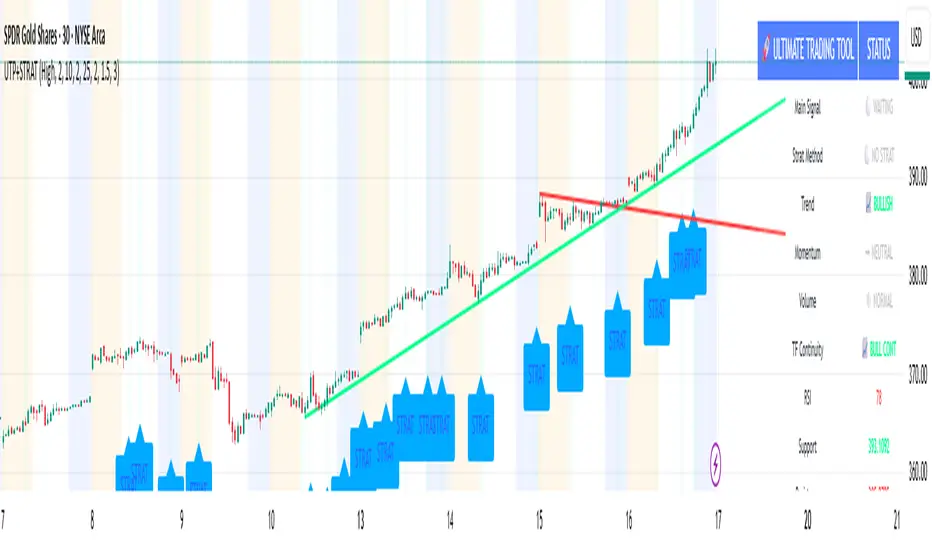
1D Exit Alerts"A Daily Exit LONG" + "B Daily Exit SHORT":
I'm not using this one anymore since they often make me worry more than necessary, and I focus more on aiming to reach specific price targets, or using the 5m Exit alerts instead.
Also swing trades require less time-sensitive operations than day trades, so for me personally they felt a bit redundant.
But maybe it helps some of you:
There are 4 conditions that trigger it. As with 5m Exit Alerts, the triggering reasons show up in the exit alert message (unfortunately only as a number, since alert messages can't have "dynamic text" in TradingView).
Here are the conditions sorted from best to worst:
Gap Up / Down. Better check SPY and the stock whether a Gap Reversal is likely to happen (aka get out) or whether the stock will keep going higher / lower.
Earnings: End of day or Tomorrow morning. Alert is triggered at beginning of morning before earnings, and then again 15m before market close.
Mental stop loss: Broke daily EMA 8 or SMA - in the wrong direction....
Wrong direction: Broke below / above yesterday's Low / High. It's not immediately triggered, but only after re-touching VWAP again, to prevent too impulsive exits.
As with 5m Exit alerts: Always consider how the market and stock looks like, then decide whether to exit or not! These are meant to make you look at the chart, not to FOMO-exit.
"X Candle Close":
Same as in 1D Enter alert: Is triggered 15m before market close (I put it in here as well because I kept forgetting whether I put this one into Enter or Exit alerts...)
More infos: www.reddit.com
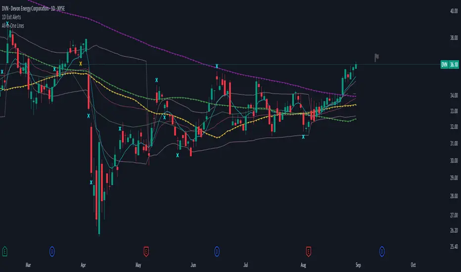
Close Above/Below Prev 2 Candle (Daily Close)This strategy identifies potential trend continuation or breakout signals by analyzing the daily candle closes relative to the previous two daily candles. It generates clear alerts and trade signals only after the daily candle has fully closed, reducing false intraday triggers.
How it works:
Long Entry (Bullish Signal): Triggered when the daily candle closes above the highs of the previous two daily candles.
Short Entry (Bearish Signal): Triggered when the daily candle closes below the lows of the previous two daily candles.
Visual Indicators: Green triangles indicate bullish signals, red triangles indicate bearish signals.
Strategy Features:
Optional long and short entries with configurable risk/reward ratio.
Automatic stop-loss and take-profit calculation based on candle structure.
Works on intraday charts using daily candle analysis.
Alerts:
Alerts trigger only after the daily candle closes above/below the previous two daily candles.
Helps traders receive precise notifications for potential breakout trades.
Benefits:
Reduces noise by using daily candle closes.
Easy to integrate with other swing or trend strategies.
Provides clear visual and alert signals for both bullish and bearish setups.
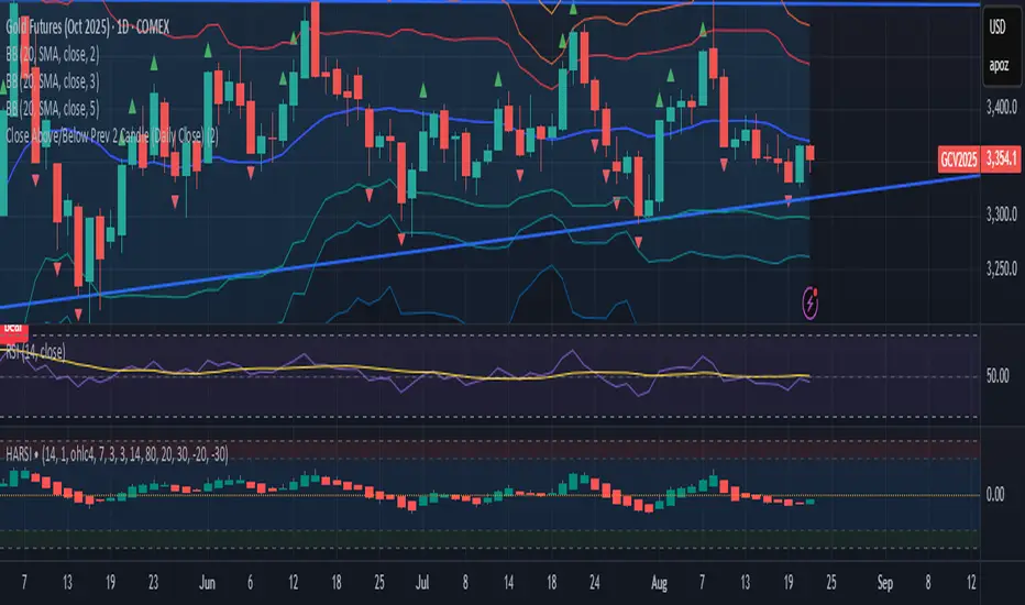
Defense Mode Dashboard ProWhat it is
A one‑look market regime dashboard for ES, NQ, YM, RTY, and SPY that tells you when to play defense, when you might have an offense cue, and when to chill. It blends VIX, VIX term structure, ATR 5 over 60, and session gap signals with clean alerts and a compact table you can park anywhere.
Why traders like it
Because it filters out the noise. Regime first, tactics second. You avoid trading size into landmines and lean in when volatility cooperates.
What it measures
Volatility stress with VIX level and VIX vs 20‑SMA
Term structure using VX1 vs VX2 with two modes
Diff mode: VX1 minus VX2
Ratio mode: VX1 divided by VX2
Realized volatility using ATR5 over ATR60 with optional smoothing
Session risk from RTH opening gaps and overnight range, normalized by ATR
How to use in 30 seconds
Pick a preset in the inputs. ES, NQ, YM, RTY, SPY are ready.
Leave thresholds at defaults to start.
Add one TradingView alert using “Any alert() function call”.
Trade smaller or stand aside when the header reads DEFENSE ON. Consider leaning in only when you see OFFENSE CUE and your playbook agrees.
Defaults we recommend
VIX triggers: 22 and 1.25× the 20‑SMA
Term mode: Diff with tolerance 0.00. Use Ratio at 1.00+ for choppier markets
ATR 5/60 defense: 1.25. Offense cue: 0.85 or lower
ATR smoothing: 1. Try 2 to 3 if you want fewer flips
Gap mode: RTH. Turn Both on if you want ON range to count too
RTH wild gap: 0.60× ATR5. ON wild range: 0.80× ATR5
Alert cadence: Once per RTH session
Snooze: Quick snooze first 30 minutes on. Fire on snooze exit off, unless you really want the catch‑up ping
New since the last description
Multi‑asset presets set symbols and RTH windows for ES, NQ, YM, RTY, SPY
Term ratio mode with near‑flat warning when ratio is between 1.00 and your trigger
ATR smoothing for the 5 over 60 ratio
RTH keying for cadence, so “Once per RTH session” behaves like a trader expects
Snooze upgrades with quick snooze tied to the first N minutes of RTH and an optional fire‑on‑snooze‑exit
Compact title merge and user color controls for labels, values, borders, and background
Exposed series for integrations: DefenseOn(1=yes) and OffenseCue(1=yes)
Debug toggle to visualize gap points, ON range, and term readings
Stronger NA handling with a clear “No core data” row when feeds are missing
Notes
Dynamic alerts require “Any alert() function call”.
Works on any chart timeframe. Daily reads and 1‑minute anchors handle the regime logic.

Gemini Trend Following SystemStrategy Description: The Gemini Trend Following System
Core Philosophy
This is a long-term trend-following system designed for a position trader or a patient swing trader, not a day trader. The fundamental goal is to capture the majority of a stock's major, multi-month or even multi-year uptrend.
The core principle is: "Buy weakness in a confirmed uptrend, and sell only when the uptrend's structure is fundamentally broken."
It operates on the belief that it's more profitable to ride a durable trend than to chase short-term breakouts or worry about daily price fluctuations. It prioritizes staying in a winning trade over frequent trading.
The Three Pillars of the Strategy
The script's logic is built on three distinct pillars, processed in order:
1. The Regime Filter: "Is This Stock in a Healthy Uptrend?"
Before even considering a trade, the script acts as a strict gatekeeper. It will only "watch" a stock if it meets all the criteria of a healthy, long-term uptrend. This is the most important part of the strategy as it filters out weak or speculative stocks.
A stock passes this filter if:
The 50-day Simple Moving Average (SMA) is above the 200-day SMA. This is the classic definition of a "Golden Cross" state, indicating the medium-term trend is stronger than the long-term trend—a hallmark of a bull market for the stock.
The stock's performance over the last year is positive. The Rate of Change (ROC) must be above a minimum threshold (e.g., 15%). This ensures we are only looking at stocks that have already demonstrated significant strength.
The 200-day SMA itself is rising. This is a crucial check to ensure the very foundation of the trend is solid and not flattening out or beginning to decline.
If a stock doesn't meet these conditions, the script ignores it completely.
2. The Entry Trigger: "When to Buy the Dip"
Once a stock is confirmed to be in a healthy uptrend, the script does not buy immediately. Instead, it patiently waits for a point of lower risk and higher potential reward—a pullback.
The entry trigger is a specific, two-step sequence:
The stock price first dips and closes below its 50-day SMA. This signifies a period of temporary weakness or profit-taking.
The price then recovers and closes back above the 50-day SMA within a short period (10 bars).
This sequence is a powerful signal. It suggests that institutional buyers view the 50-day SMA as a key support level and have stepped in to defend it, overpowering the sellers. The entry occurs at this point of confirmed support, marking the likely resumption of the uptrend. On the chart, this event is highlighted with a teal background.
3. The Exit Strategy: "When is the Trend Over?"
The exit logic is designed to keep you in the trade as long as possible and only sell when the trend's character has fundamentally changed. It uses a dual-exit system:
Primary Exit (Trend Failure): The main reason to sell is a "Death Cross"—when the 50-day SMA crosses below the 200-day SMA. This is a robust, albeit lagging, signal that the long-term uptrend is over and a bearish market structure is taking hold. This exit condition is designed to ignore normal market corrections and only trigger when the underlying trend has truly broken. On the chart, this is highlighted with a maroon background.
Safety-Net Exit (Catastrophic Stop-Loss): To protect against a sudden market crash or a company-specific disaster, a "safety-net" stop-loss is placed at the time of entry. This stop is set far below the entry price, typically underneath the 200-day SMA. It is a "just-in-case" measure that should only be triggered in a severe and rapid decline, protecting your capital from an unexpected black swan event.
Who is This Strategy For?
Position Traders: Investors who are comfortable holding a stock for many months to over a year.
Patient Swing Traders: Traders who want to capture large price swings over weeks and months, not days.
Investors using a Rules-Based Approach: Anyone looking to apply a disciplined, non-emotional system to their long-term portfolio.
Ideal Market Conditions
This strategy excels in markets with clear, durable trends. It performs best on strong, leading stocks during a sustained bull market. It will underperform significantly or generate losses in choppy, sideways, or range-bound markets, where the moving averages will frequently cross back and forth, leading to "whipsaw" trades.

NQ Phantom Scalper Pro# 👻 NQ Phantom Scalper Pro
**Advanced VWAP Mean Reversion Strategy with Volume Confirmation**
## 🎯 Strategy Overview
The NQ Phantom Scalper Pro is a sophisticated mean reversion strategy designed specifically for Nasdaq 100 (NQ) futures scalping. This strategy combines Volume Weighted Average Price (VWAP) bands with intelligent volume spike detection to identify high-probability reversal opportunities during optimal market hours.
## 🔧 Key Features
### VWAP Band System
- **Dynamic VWAP Bands**: Automatically adjusting standard deviation bands based on intraday volatility
- **Multiple Band Levels**: Configurable Band #1 (entry trigger) and Band #2 (profit target reference)
- **Flexible Anchoring**: Choose from Session, Week, Month, Quarter, or Year-based VWAP calculations
### Volume Intelligence
- **Volume Spike Detection**: Only triggers entries when volume exceeds SMA by configurable multiplier
- **Relative Volume Display**: Real-time volume strength indicator in info panel
- **Optional Volume Filter**: Can be disabled for testing alternative setups
### Advanced Time Management
- **12-Hour Format**: User-friendly time inputs (9 AM - 4 PM default)
- **Lunch Filter**: Automatically avoids low-liquidity lunch period (12-2 PM)
- **Visual Time Zones**: Color-coded background for active/inactive periods
- **Market Hours Focus**: Optimized for peak NQ trading sessions
### Smart Risk Management
- **ATR-Based Stops**: Volatility-adjusted stop losses using Average True Range
- **Dual Exit Strategy**: VWAP mean reversion + fixed profit targets
- **Adjustable Risk-Reward**: Configurable target ratio to opposite VWAP band
- **Position Sizing**: Percentage-based equity allocation
### Optional Trend Filter
- **EMA Trend Alignment**: Optional trend filter to avoid counter-trend trades
- **Configurable Period**: Adjustable EMA length for trend determination
- **Toggle Functionality**: Enable/disable based on market conditions
## 📊 How It Works
### Entry Logic
**Long Entries**: Triggered when price touches lower VWAP band + volume spike during active hours
**Short Entries**: Triggered when price touches upper VWAP band + volume spike during active hours
### Exit Strategy
1. **VWAP Mean Reversion**: Early exit when price returns to VWAP center line
2. **Profit Target**: Fixed target based on percentage to opposite VWAP band
3. **Stop Loss**: ATR-based protective stop
### Visual Elements
- **VWAP Center Line**: Blue line showing volume-weighted fair value
- **Green Bands**: Entry trigger levels (Band #1)
- **Red Bands**: Extended levels for target reference (Band #2)
- **Orange EMA**: Trend filter line (when enabled)
- **Background Colors**: Yellow (lunch), Gray (after hours), Clear (active trading)
- **Info Panel**: Real-time metrics display
## ⚙️ Recommended Settings
### Timeframes
- **Primary**: 1-5 minute charts for scalping
- **Validation**: Test on 15-minute for swing applications
### Market Conditions
- **Best Performance**: Ranging/choppy markets with good volume
- **Trend Markets**: Enable trend filter to avoid counter-trend trades
- **High Volatility**: Increase ATR multiplier for stops
### Session Optimization
- **Pre-Market**: Generally avoided (low volume)
- **Morning Session**: 9:30 AM - 12:00 PM (high activity)
- **Lunch Period**: 12:00 PM - 2:00 PM (filtered by default)
- **Afternoon Session**: 2:00 PM - 4:00 PM (good volume)
- **After Hours**: Generally avoided (wide spreads)
## ⚠️ Risk Disclaimer
This strategy is for educational purposes only and does not constitute financial advice. Past performance does not guarantee future results. Trading futures involves substantial risk of loss and is not suitable for all investors. Users should:
- Thoroughly backtest on historical data
- Start with small position sizes
- Understand the risks of leveraged trading
- Consider transaction costs and slippage
- Never risk more than you can afford to lose
## 📈 Performance Tips
1. **Volume Threshold**: Adjust volume multiplier based on average NQ volume patterns
2. **Band Sensitivity**: Modify band multipliers for different volatility regimes
3. **Time Filters**: Customize trading hours based on your timezone and preferences
4. **Trend Alignment**: Use trend filter during strong directional markets
5. **Risk Management**: Always maintain consistent position sizing and risk parameters
**Version**: 6.0 Compatible
**Asset**: Optimized for NASDAQ 100 Futures (NQ)
**Style**: Mean Reversion Scalping
**Frequency**: High-Frequency Trading Ready
ALEX - ATR Extensions + ADR + TableALEX - ATR Extensions + ADR + Table
Overview
The ALEX ATR Extensions indicator is a comprehensive volatility and momentum analysis tool that combines Average True Range (ATR), Average Daily Range (ADR), and moving average distance calculations in a single, customizable display. This indicator helps traders assess current price action relative to historical volatility and key moving averages, providing crucial context for risk management and trade planning.
Key Features
Multi-Metric Analysis
- ATR Percentage: Current ATR as a percentage of price for volatility assessment
- ADR Percentage: Average Daily Range as a percentage for typical daily movement
- Low of Day Distance: Distance from current price to daily low
- Moving Average Distance: ATR-normalized distance from 21 and 50 period moving averages
Flexible Moving Average Options
- Configurable MA Types: Choose between EMA or SMA for both 21 and 50 period averages
- Customizable Periods: Adjust moving average lengths to suit your trading style
- Daily Timeframe Data: Uses daily moving averages regardless of chart timeframe
ATR Extension Levels
- Dynamic Price Targets: Calculate extension levels based on ATR multiples from moving averages
- Visual Reference Lines: Optional overlay lines showing ATR extension targets
- Customizable Multipliers: Adjust ATR multipliers for different risk/reward scenarios
Smart Visual Alerts
- Color-Coded Distance Metrics: Automatic color changes based on distance thresholds
- Symbol Plotting: Customizable chart symbols when distance thresholds are exceeded
- Threshold-Based Alerts: Visual cues when price reaches significant ATR distances
Comprehensive Data Table
- Real-Time Metrics: Live updating table with all key measurements
- Customizable Display: Toggle individual metrics on/off based on preference
- Professional Styling: Adjustable colors, fonts, and transparency
How to Use
Volatility Assessment
- High ATR%: Indicates elevated volatility, larger position sizing considerations
- Low ATR%: Suggests compressed volatility, potential for expansion
- ADR% Comparison: Compare current day's range to historical average
Moving Average Analysis
- ATR Distance 21/50: Normalized distance showing how extended price is from key levels
- Positive Values: Price above moving average (bullish positioning)
- Negative Values: Price below moving average (bearish positioning)
- Color Changes: Automatic alerts when reaching threshold levels
Extension Target Planning
- ATR Extension Lines: Visual price targets based on volatility-adjusted projections
- Risk/Reward Planning: Use extension levels for profit target placement
- Breakout Confirmation: Extension levels can confirm breakout validity
Symbol Alert System
- Chart Symbols: Automatic plotting when distance thresholds are breached
- Customizable Triggers: Set your own threshold levels for alerts
- Visual Scanning: Quick identification of extended conditions across multiple charts
Settings
Display Controls
- Show ADR%: Toggle average daily range percentage display
- Show ATR%: Toggle average true range percentage display
- Show LoD Distance: Toggle low of day distance calculation
- Show LoD Price: Toggle actual low of day price display
- Show ATR Distance from 21/50 DMA: Toggle moving average distance metrics
- Show 21/50 DMA Price: Toggle actual moving average price display
- Show ATR Extension Levels: Toggle extension target display in table
Moving Average Configuration
- 21/50 DMA Type: Choose between EMA or SMA calculation methods
- 21/50 DMA Period: Customize moving average lengths
- ADR/ATR Length: Adjust calculation periods for range measurements
Color Thresholds
- Threshold Levels: Set distance levels for color changes (default 2.0 and 5.0)
- Custom Colors: Choose colors for different threshold breaches
- Separate 21/50 Settings: Independent color schemes for each moving average
Symbol Settings
- Show Char Symbol: Toggle symbol plotting for each moving average
- Custom Symbols: Choose any character for chart plotting
- Symbol Colors: Customize colors for visual distinction
- Threshold Levels: Set trigger points for symbol appearance
ATR Extension Lines
- Show Extension Lines: Toggle visual extension level lines
- ATR Multipliers: Customize extension distance (default 2.0x)
- Line Colors: Choose colors for extension level visualization
Table Customization
- Background Color: Adjust table transparency and color
- Text Color: Customize default text appearance
- Font Size: Choose from tiny to huge font options
Advanced Applications
Trend Strength Analysis
- Large ATR distances suggest strong trending moves
- Small ATR distances indicate potential consolidation or reversal zones
- Compare current readings to recent historical ranges
Risk Management
- Use ATR% for position sizing calculations
- Extension levels provide natural profit target zones
- Distance metrics help identify overextended conditions
Multi-Timeframe Context
- Apply to different timeframes for comprehensive analysis
- Daily data provides consistency across all chart intervals
- Combine with weekly/monthly analysis for broader context
Market Regime Identification
- High volatility periods: Increased ATR% readings
- Low volatility periods: Compressed ATR% readings
- Trending markets: Sustained high distance readings
- Consolidating markets: Low distance readings with frequent color changes
Best Practices
Volatility-Adjusted Trading
- Increase position sizes during low volatility periods
- Reduce position sizes during high volatility periods
- Use ATR% for stop-loss placement relative to normal market movement
Extension Level Usage
- Primary targets: 1.5-2.0x ATR extensions
- Secondary targets: 2.5-3.0x ATR extensions
- Avoid chasing prices beyond 3x ATR extensions
Threshold Optimization
- Backtest different threshold levels for your trading style
- Consider market conditions when setting alert levels
- Adjust thresholds based on instrument volatility characteristics
Integration Strategies
- Combine with momentum indicators for confirmation
- Use alongside support/resistance levels
- Incorporate into systematic trading approaches
Technical Specifications
- Compatible with Pine Script v6
- Uses daily timeframe data for consistency
- Optimized for real-time performance
- Works on all chart types and timeframes
- Supports all tradeable instruments
Ideal For
- Swing traders using daily charts
- Position traders seeking volatility context
- Day traders needing intraday reference levels
- Risk managers requiring volatility metrics
- Systematic traders building rule-based strategies
Disclaimer
This indicator is for educational and informational purposes only. It should not be used as the sole basis for trading decisions. Always combine with other forms of analysis, proper risk management techniques, and consider your individual trading plan and risk tolerance. Past performance does not guarantee future results.
Compatible with Pine Script v6 | Optimized for daily timeframe analysis | Works across all markets and instruments

Quarterly Theory ICT 05 [TradingFinder] Doubling Theory Signals🔵 Introduction
Doubling Theory is an advanced approach to price action and market structure analysis that uniquely combines time-based analysis with key Smart Money concepts such as SMT (Smart Money Technique), SSMT (Sequential SMT), Liquidity Sweep, and the Quarterly Theory ICT.
By leveraging fractal time structures and precisely identifying liquidity zones, this method aims to reveal institutional activity specifically smart money entry and exit points hidden within price movements.
At its core, the market is divided into two structural phases: Doubling 1 and Doubling 2. Each phase contains four quarters (Q1 through Q4), which follow the logic of the Quarterly Theory: Accumulation, Manipulation (Judas Swing), Distribution, and Continuation/Reversal.
These segments are anchored by the True Open, allowing for precise alignment with cyclical market behavior and providing a deeper structural interpretation of price action.
During Doubling 1, a Sequential SMT (SSMT) Divergence typically forms between two correlated assets. This time-structured divergence occurs between two swing points positioned in separate quarters (e.g., Q1 and Q2), where one asset breaks a significant low or high, while the second asset fails to confirm it. This lack of confirmation—especially when aligned with the Manipulation and Accumulation phases—often signals early smart money involvement.
Following this, the highest and lowest price points from Doubling 1 are designated as liquidity zones. As the market transitions into Doubling 2, it commonly returns to these zones in a calculated move known as a Liquidity Sweep—a sharp, engineered spike intended to trigger stop orders and pending positions. This sweep, often orchestrated by institutional players, facilitates entry into large positions with minimal slippage.
Bullish :
Bearish :
🔵 How to Use
Applying Doubling Theory requires a simultaneous understanding of temporal structure and inter-asset behavioral divergence. The method unfolds over two main phases—Doubling 1 and Doubling 2—each divided into four quarters (Q1 to Q4).
The first phase focuses on identifying a Sequential SMT (SSMT) divergence, which forms when two correlated assets (e.g., EURUSD and GBPUSD, or NQ and ES) react differently to key price levels across distinct quarters. For example, one asset may break a previous low while the other maintains structure. This misalignment—especially in Q2, the Manipulation phase—often indicates early smart money accumulation or distribution.
Once this divergence is observed, the extreme highs and lows of Doubling 1 are marked as liquidity zones. In Doubling 2, the market gravitates back toward these zones, executing a Liquidity Sweep.
This move is deliberate—designed to activate clustered stop-loss and pending orders and to exploit pockets of resting liquidity. These sweeps are typically driven by institutional forces looking to absorb liquidity and position themselves ahead of the next major price move.
The key to execution lies in the fact that, during the sweep in Doubling 2, a classic SMT divergence should also appear between the two assets. This indicates a weakening of the previous trend and adds an extra layer of confirmation.
🟣 Bullish Doubling Theory
In the bullish scenario, Doubling 1 begins with a bullish SSMT divergence, where one asset forms a lower low while the other maintains its structure. This divergence signals weakening bearish momentum and possible smart money accumulation. In Doubling 2, the market returns to the previous low and sweeps the liquidity zone—breaking below it on one asset, while the second fails to confirm, forming a bullish SMT divergence.
f this move is followed by a bullish PSP and a clear market structure break (MSB), a long entry is triggered. The stop-loss is placed just below the swept liquidity zone, while the target is set in the premium zone, anticipating a move driven by institutional buyers.
🟣 Bearish Doubling Theory
The bearish scenario follows the same structure in reverse. In Doubling 1, a bearish SSMT divergence occurs when one asset prints a higher high while the other fails to do so. This suggests distribution and weakening buying pressure. Then, in Doubling 2, the market returns to the previous high and executes a liquidity sweep, targeting trapped buyers.
A bearish SMT divergence appears, confirming the move, followed by a bearish PSP on the lower timeframe. A short position is initiated after a confirmed MSB, with the stop-loss placed
🔵 Settings
⚙️ Logical Settings
Quarterly Cycles Type : Select the time segmentation method for SMT analysis.
Available modes include : Yearly, Monthly, Weekly, Daily, 90 Minute, and Micro.
These define how the indicator divides market time into Q1–Q4 cycles.
Symbol : Choose the secondary asset to compare with the main chart asset (e.g., XAUUSD, US100, GBPUSD).
Pivot Period : Sets the sensitivity of the pivot detection algorithm. A smaller value increases responsiveness to price swings.
Pivot Sync Threshold : The maximum allowed difference (in bars) between pivots of the two assets for them to be compared.
Validity Pivot Length : Defines the time window (in bars) during which a divergence remains valid before it's considered outdated.
🎨 Display Settings
Show Cycle :Toggles the visual display of the current Quarter (Q1 to Q4) based on the selected time segmentation
Show Cycle Label : Shows the name (e.g., "Q2") of each detected Quarter on the chart.
Show Labels : Displays dynamic labels (e.g., “Q2”, “Bullish SMT”, “Sweep”) at relevant points.
Show Lines : Draws connection lines between key pivot or divergence points.
Color Settings : Allows customization of colors for bullish and bearish elements (lines, labels, and shapes)
🔔 Alert Settings
Alert Name : Custom name for the alert messages (used in TradingView’s alert system).
Message Frequenc y:
All : Every signal triggers an alert.
Once Per Bar : Alerts once per bar regardless of how many signals occur.
Per Bar Close : Only triggers when the bar closes and the signal still exists.
Time Zone Display : Choose the time zone in which alert timestamps are displayed (e.g., UTC).
Bullish SMT Divergence Alert : Enable/disable alerts specifically for bullish signals.
Bearish SMT Divergence Alert : Enable/disable alerts specifically for bearish signals
🔵 Conclusion
Doubling Theory is a powerful and structured framework within the realm of Smart Money Concepts and ICT methodology, enabling traders to detect high-probability reversal points with precision. By integrating SSMT, SMT, Liquidity Sweeps, and the Quarterly Theory into a unified system, this approach shifts the focus from reactive trading to anticipatory analysis—anchored in time, structure, and liquidity.
What makes Doubling Theory stand out is its logical synergy of time cycles, behavioral divergence, liquidity targeting, and institutional confirmation. In both bullish and bearish scenarios, it provides clearly defined entry and exit strategies, allowing traders to engage the market with confidence, controlled risk, and deeper insight into the mechanics of price manipulation and smart money footprints.
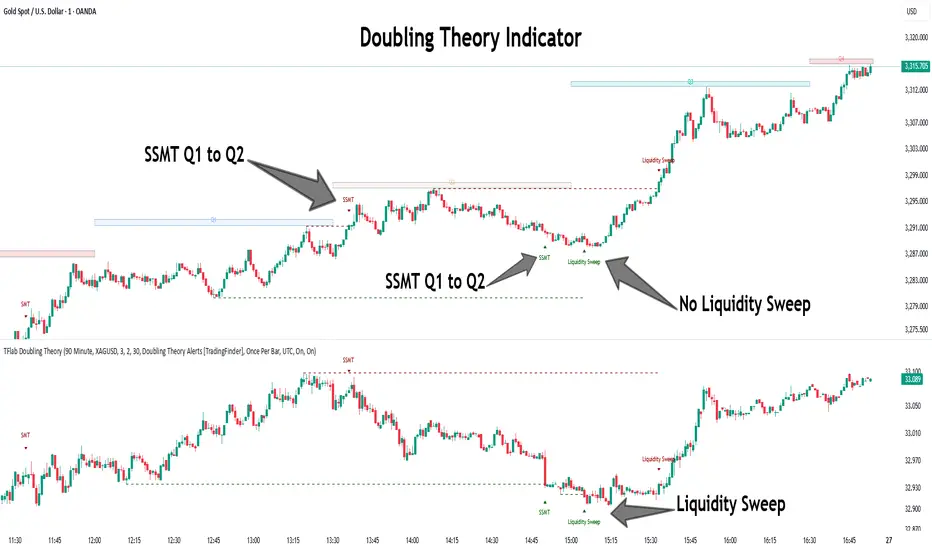
Smart Liquidity Wave [The_lurker]"Smart Liquidity Wave" هو مؤشر تحليلي متطور يهدف لتحديد نقاط الدخول والخروج المثلى بناءً على تحليل السيولة، قوة الاتجاه، وإشارات السوق المفلترة. يتميز المؤشر بقدرته على تصنيف الأدوات المالية إلى أربع فئات سيولة (ضعيفة، متوسطة، عالية، عالية جدًا)، مع تطبيق شروط مخصصة لكل فئة تعتمد على تحليل الموجات السعرية، الفلاتر المتعددة، ومؤشر ADX.
فكرة المؤشر
الفكرة الأساسية هي الجمع بين قياس السيولة اليومية الثابتة وتحليل ديناميكي للسعر باستخدام فلاتر متقدمة لتوليد إشارات دقيقة. المؤشر يركز على تصفية الضوضاء في السوق من خلال طبقات متعددة من التحليل، مما يجعله أداة ذكية تتكيف مع الأدوات المالية المختلفة بناءً على مستوى سيولتها.
طريقة عمل المؤشر
1- قياس السيولة:
يتم حساب السيولة باستخدام متوسط حجم التداول على مدى 14 يومًا مضروبًا في سعر الإغلاق، ويتم ذلك دائمًا على الإطار الزمني اليومي لضمان ثبات القيمة بغض النظر عن الإطار الزمني المستخدم في الرسم البياني.
يتم تصنيف السيولة إلى:
ضعيفة: أقل من 5 ملايين (قابل للتعديل).
متوسطة: من 5 إلى 20 مليون.
عالية: من 20 إلى 50 مليون.
عالية جدًا: أكثر من 50 مليون.
هذا الثبات في القياس يضمن أن تصنيف السيولة لا يتغير مع تغير الإطار الزمني، مما يوفر أساسًا موثوقًا للإشارات.
2- تحليل الموجات السعرية:
يعتمد المؤشر على تحليل الموجات باستخدام متوسطات متحركة متعددة الأنواع (مثل SMA، EMA، WMA، HMA، وغيرها) يمكن للمستخدم اختيارها وتخصيص فتراتها ، يتم دمج هذا التحليل مع مؤشرات إضافية مثل RSI (مؤشر القوة النسبية) وMFI (مؤشر تدفق الأموال) بوزن محدد (40% للموجات، 30% لكل من RSI وMFI) للحصول على تقييم شامل للاتجاه.
3- الفلاتر وطريقة عملها:
المؤشر يستخدم نظام فلاتر متعدد الطبقات لتصفية الإشارات وتقليل الضوضاء، وهي من أبرز الجوانب المخفية التي تعزز دقته:
الفلتر الرئيسي (Main Filter):
يعمل على تنعيم التغيرات السعرية السريعة باستخدام معادلة رياضية تعتمد على تحليل الإشارات (Signal Processing).
يتم تطبيقه على السعر لاستخراج الاتجاهات الأساسية بعيدًا عن التقلبات العشوائية، مع فترة زمنية قابلة للتعديل (افتراضي: 30).
يستخدم تقنية مشابهة للفلاتر عالية التردد (High-Pass Filter) للتركيز على الحركات الكبيرة.
الفلتر الفرعي (Sub Filter):
يعمل كطبقة ثانية للتصفية، مع فترة أقصر (افتراضي: 12)، لضبط الإشارات بدقة أكبر.
يستخدم معادلات تعتمد على الترددات المنخفضة للتأكد من أن الإشارات الناتجة تعكس تغيرات حقيقية وليست مجرد ضوضاء.
إشارة الزناد (Signal Trigger):
يتم تطبيق متوسط متحرك على نتائج الفلتر الرئيسي لتوليد خط إشارة (Signal Line) يُقارن مع عتبات محددة للدخول والخروج.
يمكن تعديل فترة الزناد (افتراضي: 3 للدخول، 5 للخروج) لتسريع أو تبطيء الإشارات.
الفلتر المربع (Square Filter):
خاصية مخفية تُفعّل افتراضيًا تعزز دقة الفلاتر عن طريق تضييق نطاق التذبذبات المسموح بها، مما يقلل من الإشارات العشوائية في الأسواق المتقلبة.
4- تصفية الإشارات باستخدام ADX:
يتم استخدام مؤشر ADX كفلتر نهائي للتأكد من قوة الاتجاه قبل إصدار الإشارة:
ضعيفة ومتوسطة: دخول عندما يكون ADX فوق 40، خروج فوق 50.
عالية: دخول فوق 40، خروج فوق 55.
عالية جدًا: دخول فوق 35، خروج فوق 38.
هذه العتبات قابلة للتعديل، مما يسمح بتكييف المؤشر مع استراتيجيات مختلفة.
5- توليد الإشارات:
الدخول: يتم إصدار إشارة شراء عندما تنخفض خطوط الإشارة إلى ما دون عتبة محددة (مثل -9) مع تحقق شروط الفلاتر، السيولة، وADX.
الخروج: يتم إصدار إشارة بيع عندما ترتفع الخطوط فوق عتبة (مثل 109 أو 106 حسب الفئة) مع تحقق الشروط الأخرى.
تُعرض الإشارات بألوان مميزة (أزرق للدخول، برتقالي للضعيفة والمتوسطة، أحمر للعالية والعالية جدًا) وبثلاثة أحجام (صغير، متوسط، كبير).
6- عرض النتائج:
يظهر مستوى السيولة الحالي في جدول في أعلى يمين الرسم البياني، مما يتيح للمستخدم معرفة فئة الأصل بسهولة.
7- دعم التنبيهات:
تنبيهات فورية لكل فئة سيولة، مما يسهل التداول الآلي أو اليدوي.
%%%%% الجوانب المخفية في الكود %%%%%
معادلات الفلاتر المتقدمة: يستخدم المؤشر معادلات رياضية معقدة مستوحاة من معالجة الإشارات لتنعيم البيانات واستخراج الاتجاهات، مما يجعله أكثر دقة من المؤشرات التقليدية.
التكيف التلقائي: النظام يضبط نفسه داخليًا بناءً على التغيرات في السعر والحجم، مع عوامل تصحيح مخفية (مثل معامل التنعيم في الفلاتر) للحفاظ على الاستقرار.
التوزيع الموزون: الدمج بين الموجات، RSI، وMFI يتم بأوزان محددة (40%، 30%، 30%) لضمان توازن التحليل، وهي تفاصيل غير ظاهرة مباشرة للمستخدم لكنها تؤثر على النتائج.
الفلتر المربع: خيار مخفي يتم تفعيله افتراضيًا لتضييق نطاق الإشارات، مما يقلل من التشتت في الأسواق ذات التقلبات العالية.
مميزات المؤشر
1- فلاتر متعددة الطبقات: تضمن تصفية الضوضاء وإنتاج إشارات موثوقة فقط.
2- ثبات السيولة: قياس السيولة اليومي يجعل التصنيف متسقًا عبر الإطارات الزمنية.
3- تخصيص شامل: يمكن تعديل حدود السيولة، عتبات ADX، فترات الفلاتر، وأنواع المتوسطات المتحركة.
4- إشارات مرئية واضحة: تصميم بصري يسهل التفسير مع تنبيهات فورية.
5- تقليل الإشارات الخاطئة: الجمع بين الفلاتر وADX يعزز الدقة ويقلل من التشتت.
إخلاء المسؤولية
لا يُقصد بالمعلومات والمنشورات أن تكون، أو تشكل، أي نصيحة مالية أو استثمارية أو تجارية أو أنواع أخرى من النصائح أو التوصيات المقدمة أو المعتمدة من TradingView.
#### **What is the Smart Liquidity Wave Indicator?**
"Smart Liquidity Wave" is an advanced analytical indicator designed to identify optimal entry and exit points based on liquidity analysis, trend strength, and filtered market signals. It stands out with its ability to categorize financial instruments into four liquidity levels (Weak, Medium, High, Very High), applying customized conditions for each category based on price wave analysis, multi-layered filters, and the ADX (Average Directional Index).
#### **Concept of the Indicator**
The core idea is to combine a stable daily liquidity measurement with dynamic price analysis using sophisticated filters to generate precise signals. The indicator focuses on eliminating market noise through multiple analytical layers, making it an intelligent tool that adapts to various financial instruments based on their liquidity levels.
#### **How the Indicator Works**
1. **Liquidity Measurement:**
- Liquidity is calculated using the 14-day average trading volume multiplied by the closing price, always based on the daily timeframe to ensure value consistency regardless of the chart’s timeframe.
- Liquidity is classified as:
- **Weak:** Less than 5 million (adjustable).
- **Medium:** 5 to 20 million.
- **High:** 20 to 50 million.
- **Very High:** Over 50 million.
- This consistency in measurement ensures that liquidity classification remains unchanged across different timeframes, providing a reliable foundation for signals.
2. **Price Wave Analysis:**
- The indicator relies on wave analysis using various types of moving averages (e.g., SMA, EMA, WMA, HMA, etc.), which users can select and customize in terms of periods.
- This analysis is integrated with additional indicators like RSI (Relative Strength Index) and MFI (Money Flow Index), weighted specifically (40% waves, 30% RSI, 30% MFI) to provide a comprehensive trend assessment.
3. **Filters and Their Functionality:**
- The indicator employs a multi-layered filtering system to refine signals and reduce noise, a key hidden feature that enhances its accuracy:
- **Main Filter:**
- Smooths rapid price fluctuations using a mathematical equation rooted in signal processing techniques.
- Applied to price data to extract core trends away from random volatility, with an adjustable period (default: 30).
- Utilizes a technique similar to high-pass filters to focus on significant movements.
- **Sub Filter:**
- Acts as a secondary filtering layer with a shorter period (default: 12) for finer signal tuning.
- Employs low-frequency-based equations to ensure resulting signals reflect genuine changes rather than mere noise.
- **Signal Trigger:**
- Applies a moving average to the main filter’s output to generate a signal line, compared against predefined entry and exit thresholds.
- Trigger period is adjustable (default: 3 for entry, 5 for exit) to speed up or slow down signals.
- **Square Filter:**
- A hidden feature activated by default, enhancing filter precision by narrowing the range of permissible oscillations, reducing random signals in volatile markets.
4. **Signal Filtering with ADX:**
- ADX is used as a final filter to confirm trend strength before issuing signals:
- **Weak and Medium:** Entry when ADX exceeds 40, exit above 50.
- **High:** Entry above 40, exit above 55.
- **Very High:** Entry above 35, exit above 38.
- These thresholds are adjustable, allowing the indicator to adapt to different trading strategies.
5. **Signal Generation:**
- **Entry:** A buy signal is triggered when signal lines drop below a specific threshold (e.g., -9) and conditions for filters, liquidity, and ADX are met.
- **Exit:** A sell signal is issued when signal lines rise above a threshold (e.g., 109 or 106, depending on the category) with all conditions satisfied.
- Signals are displayed in distinct colors (blue for entry, orange for Weak/Medium, red for High/Very High) and three sizes (small, medium, large).
6. **Result Display:**
- The current liquidity level is shown in a table at the top-right of the chart, enabling users to easily identify the asset’s category.
7. **Alert Support:**
- Instant alerts are provided for each liquidity category, facilitating both automated and manual trading.
#### **Hidden Aspects in the Code**
- **Advanced Filter Equations:** The indicator uses complex mathematical formulas inspired by signal processing to smooth data and extract trends, making it more precise than traditional indicators.
- **Automatic Adaptation:** The system internally adjusts based on price and volume changes, with hidden correction factors (e.g., smoothing coefficients in filters) to maintain stability.
- **Weighted Distribution:** The integration of waves, RSI, and MFI uses fixed weights (40%, 30%, 30%) for balanced analysis, a detail not directly visible but impactful on results.
- **Square Filter:** A hidden option, enabled by default, narrows signal range to minimize dispersion in high-volatility markets.
#### **Indicator Features**
1. **Multi-Layered Filters:** Ensures noise reduction and delivers only reliable signals.
2. **Liquidity Stability:** Daily liquidity measurement keeps classification consistent across timeframes.
3. **Comprehensive Customization:** Allows adjustments to liquidity thresholds, ADX levels, filter periods, and moving average types.
4. **Clear Visual Signals:** User-friendly design with easy-to-read visuals and instant alerts.
5. **Reduced False Signals:** Combining filters and ADX enhances accuracy and minimizes clutter.
#### **Disclaimer**
The information and publications are not intended to be, nor do they constitute, financial, investment, trading, or other types of advice or recommendations provided or endorsed by TradingView.
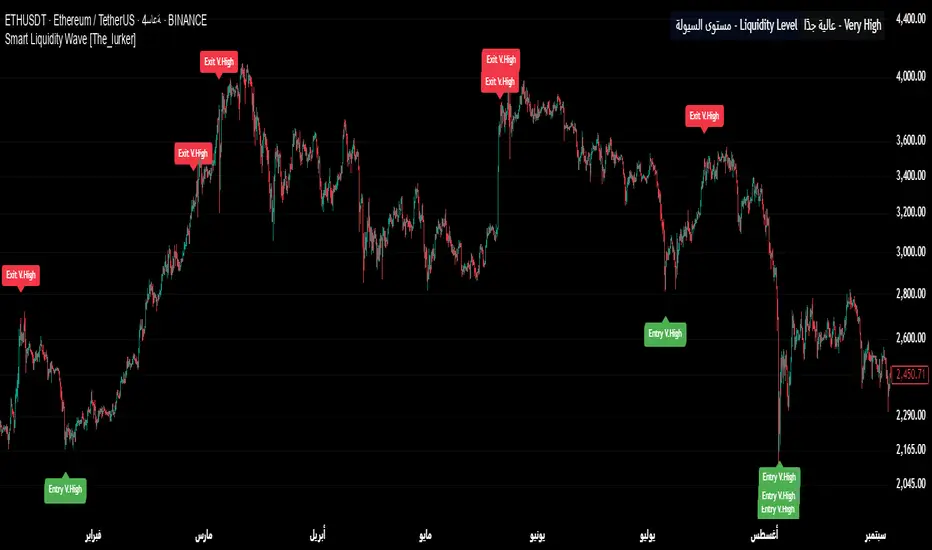
Supertrend + MACD Trend Change with AlertsDetailed Guide
1. Indicator Overview
Purpose:
This script combines the Supertrend and MACD indicators to help you detect potential trend changes. It plots a Supertrend line (green for bullish, red for bearish) and marks the chart with shapes when a trend reversal is signaled by both indicators. In addition, it includes alert conditions so that you can be notified when a potential trend change occurs.
How It Works:
Supertrend: Uses the Average True Range (ATR) to determine dynamic support and resistance levels. When the price crosses these levels, it signals a possible change in trend.
MACD: Focuses on the crossover between the MACD line and the signal line. A bullish crossover (MACD line crossing above the signal line) suggests upward momentum, while a bearish crossover (MACD line crossing below the signal line) suggests downward momentum.
2. Supertrend Component
Key Parameters:
Factor:
Function: Multiplies the ATR to create an offset from the mid-price (hl2).
Adjustment Impact: Lower values make the indicator more sensitive (producing more frequent signals), while higher values result in fewer, more confirmed signals.
ATR Period:
Function: Sets the number of bars over which the ATR is calculated.
Adjustment Impact: A shorter period makes the ATR react more quickly to recent price changes (but can be noisy), whereas a longer period provides a smoother volatility measurement.
Trend Calculation:
The script compares the previous close with the dynamically calculated upper and lower bands. If the previous close is above the upper band, the trend is set to bullish (1); if it’s below the lower band, the trend is bearish (-1). The Supertrend line is then plotted in green for bullish trends and red for bearish trends.
3. MACD Component
Key Parameters:
Fast MA (Fast Moving Average):
Function: Represents a shorter-term average, making the MACD line more sensitive to recent price movements.
Slow MA (Slow Moving Average):
Function: Represents a longer-term average to smooth out the MACD line.
Signal Smoothing:
Function: Defines the period for the signal line, which is a smoothed version of the MACD line.
Crossover Logic:
The script uses the crossover() function to detect when the MACD line crosses above the signal line (bullish crossover) and crossunder() to detect when it crosses below (bearish crossover).
4. Combined Signal Logic
How Signals Are Combined:
Bullish Scenario:
When the MACD shows a bullish crossover (MACD line crosses above the signal line) and the Supertrend indicates a bullish trend (green line), a green upward triangle is plotted below the bar.
Bearish Scenario:
When the MACD shows a bearish crossover (MACD line crosses below the signal line) and the Supertrend indicates a bearish trend (red line), a red downward triangle is plotted above the bar.
Rationale:
By combining the signals from both indicators, you increase the likelihood that the detected trend change is reliable, filtering out some false signals.
5. Alert Functionality
Alert Setup in the Code:
The alertcondition() function is used to define conditions under which TradingView can trigger alerts.
There are two alert conditions:
Bullish Alert: Activated when there is a bullish MACD crossover and the Supertrend confirms an uptrend.
Bearish Alert: Activated when there is a bearish MACD crossover and the Supertrend confirms a downtrend.
What Happens When an Alert Triggers:
When one of these conditions is met, TradingView registers the alert condition. You can then create an alert in TradingView (using the alert dialog) and choose one of these alert conditions. Once set up, you’ll receive notifications (via pop-ups, email, or SMS, depending on your settings) whenever a trend change is signaled.
6. User Adjustments and Their Effects
Factor (Supertrend):
Adjustment: Lowering the factor increases sensitivity, resulting in more frequent signals; raising it will filter out some signals, making them potentially more reliable.
ATR Period (Supertrend):
Adjustment: A shorter ATR period makes the indicator more responsive to recent price movements (but can introduce noise), while a longer period smooths out the response.
MACD Parameters (Fast MA, Slow MA, and Signal Smoothing):
Adjustment:
Shortening the Fast MA increases sensitivity, generating earlier signals that might be less reliable.
Lengthening the Slow MA produces a smoother MACD line, reducing noise.
Adjusting the Signal Smoothing changes how quickly the signal line responds to changes in the MACD line.
7. Best Practices and Considerations
Multiple Confirmation:
Even if both indicators signal a trend change, consider confirming with additional analysis such as volume, price action, or other indicators.
Market Conditions:
These indicators tend to perform best in trending markets. In sideways or choppy conditions, you may experience more false alerts.
Backtesting:
Before applying the indicator in live trading, backtest your settings to ensure they suit your trading style and the market conditions.
Risk Management:
Always use proper risk management, including stop-loss orders and appropriate position sizing, as alerts may occasionally produce late or false signals.
Happy trading!

[SHORT ONLY] ATR Sell the Rip Mean Reversion Strategy█ STRATEGY DESCRIPTION
The "ATR Sell the Rip Mean Reversion Strategy" is a contrarian system that targets overextended price moves on stocks and ETFs. It calculates an ATR‐based trigger level to identify shorting opportunities. When the current close exceeds this smoothed ATR trigger, and if the close is below a 200-period EMA (if enabled), the strategy initiates a short entry, aiming to profit from an anticipated corrective pullback.
█ HOW IS THE ATR SIGNAL BAND CALCULATED?
This strategy computes an ATR-based signal trigger as follows:
Calculate the ATR
The strategy computes the Average True Range (ATR) using a configurable period provided by the user:
atrValue = ta.atr(atrPeriod)
Determine the Threshold
Multiply the ATR by a predefined multiplier and add it to the current close:
atrThreshold = close + atrValue * atrMultInput
Smooth the Threshold
Apply a Simple Moving Average over a specified period to smooth out the threshold, reducing noise:
signalTrigger = ta.sma(atrThreshold, smoothPeriodInput)
█ SIGNAL GENERATION
1. SHORT ENTRY
A Short Signal is triggered when:
The current close is above the smoothed ATR signal trigger.
The trade occurs within the specified trading window (between Start Time and End Time).
If the EMA filter is enabled, the close must also be below the 200-period EMA.
2. EXIT CONDITION
An exit Signal is generated when the current close falls below the previous bar’s low (close < low ), indicating a potential bearish reversal and prompting the strategy to close its short position.
█ ADDITIONAL SETTINGS
ATR Period: The period used to calculate the ATR, allowing for adaptability to different volatility conditions (default is 20).
ATR Multiplier: The multiplier applied to the ATR to determine the raw threshold (default is 1.0).
Smoothing Period: The period over which the raw ATR threshold is smoothed using an SMA (default is 10).
Start Time and End Time: Defines the time window during which trades are allowed.
EMA Filter (Optional): When enabled, short entries are only executed if the current close is below the 200-period EMA, confirming a bearish trend.
█ PERFORMANCE OVERVIEW
This strategy is designed for use on the Daily timeframe, targeting stocks and ETFs by capitalizing on overextended price moves.
It utilizes a dynamic, ATR-based trigger to identify when prices have potentially peaked, setting the stage for a mean reversion short entry.
The optional EMA filter helps align trades with broader market trends, potentially reducing false signals.
Backtesting is recommended to fine-tune the ATR multiplier, smoothing period, and EMA settings to match the volatility and behavior of specific markets.

Big Candle Identifier with RSI Divergence and Advanced Stops1. Strategy Objective
The main goal of this strategy is to:
Identify significant price momentum (big candles).
Enter trades at opportune moments based on market signals (candlestick patterns and RSI divergence).
Limit initial risk through a fixed stop loss.
Maximize profits by using a trailing stop that activates only after the trade moves a specified distance in the profitable direction.
2. Components of the Strategy
A. Big Candle Identification
The strategy identifies big candles as indicators of strong momentum.
A big candle is defined as:
The body (absolute difference between close and open) of the current candle (body0) is larger than the bodies of the last five candles.
The candle is:
Bullish Big Candle: If close > open.
Bearish Big Candle: If open > close.
Purpose: Big candles signal potential continuation or reversal of trends, serving as the primary entry trigger.
B. RSI Divergence
Relative Strength Index (RSI): A momentum oscillator used to detect overbought/oversold conditions and divergence.
Fast RSI: A 5-period RSI, which is more sensitive to short-term price movements.
Slow RSI: A 14-period RSI, which smoothens fluctuations over a longer timeframe.
Divergence: The difference between the fast and slow RSIs.
Positive divergence (divergence > 0): Bullish momentum.
Negative divergence (divergence < 0): Bearish momentum.
Visualization: The divergence is plotted on the chart, helping traders confirm momentum shifts.
C. Stop Loss
Initial Stop Loss:
When entering a trade, an immediate stop loss of 200 points is applied.
This stop loss ensures the maximum risk is capped at a predefined level.
Implementation:
Long Trades: Stop loss is set below the entry price at low - 200 points.
Short Trades: Stop loss is set above the entry price at high + 200 points.
Purpose:
Prevents significant losses if the price moves against the trade immediately after entry.
D. Trailing Stop
The trailing stop is a dynamic risk management tool that adjusts with price movements to lock in profits. Here’s how it works:
Activation Condition:
The trailing stop only starts trailing when the trade moves 200 ticks (profit) in the right direction:
Long Position: close - entry_price >= 200 ticks.
Short Position: entry_price - close >= 200 ticks.
Trailing Logic:
Once activated, the trailing stop:
For Long Positions: Trails behind the price by 150 ticks (trail_stop = close - 150 ticks).
For Short Positions: Trails above the price by 150 ticks (trail_stop = close + 150 ticks).
Exit Condition:
The trade exits automatically if the price touches the trailing stop level.
Purpose:
Ensures profits are locked in as the trade progresses while still allowing room for price fluctuations.
E. Trade Entry Logic
Long Entry:
Triggered when a bullish big candle is identified.
Stop loss is set at low - 200 points.
Short Entry:
Triggered when a bearish big candle is identified.
Stop loss is set at high + 200 points.
F. Trade Exit Logic
Trailing Stop: Automatically exits the trade if the price touches the trailing stop level.
Fixed Stop Loss: Exits the trade if the price hits the predefined stop loss level.
G. 21 EMA
The strategy includes a 21-period Exponential Moving Average (EMA), which acts as a trend filter.
EMA helps visualize the overall market direction:
Price above EMA: Indicates an uptrend.
Price below EMA: Indicates a downtrend.
H. Visualization
Big Candle Identification:
The open and close prices of big candles are plotted for easy reference.
Trailing Stop:
Plotted on the chart to visualize its progression during the trade.
Green Line: Indicates the trailing stop for long positions.
Red Line: Indicates the trailing stop for short positions.
RSI Divergence:
Positive divergence is shown in green.
Negative divergence is shown in red.
3. Key Parameters
trail_start_ticks: The number of ticks required before the trailing stop activates (default: 200 ticks).
trail_distance_ticks: The distance between the trailing stop and price once the trailing stop starts (default: 150 ticks).
initial_stop_loss_points: The fixed stop loss in points applied at entry (default: 200 points).
tick_size: Automatically calculates the minimum tick size for the trading instrument.
4. Workflow of the Strategy
Step 1: Entry Signal
The strategy identifies a big candle (bullish or bearish).
If conditions are met, a trade is entered with a fixed stop loss.
Step 2: Initial Risk Management
The trade starts with an initial stop loss of 200 points.
Step 3: Trailing Stop Activation
If the trade moves 200 ticks in the profitable direction:
The trailing stop is activated and follows the price at a distance of 150 ticks.
Step 4: Exit the Trade
The trade is exited if:
The price hits the trailing stop.
The price hits the initial stop loss.
5. Advantages of the Strategy
Risk Management:
The fixed stop loss ensures that losses are capped.
The trailing stop locks in profits after the trade becomes profitable.
Momentum-Based Entries:
The strategy uses big candles as entry triggers, which often indicate strong price momentum.
Divergence Confirmation:
RSI divergence helps validate momentum and avoid false signals.
Dynamic Profit Protection:
The trailing stop adjusts dynamically, allowing the trade to capture larger moves while protecting gains.
6. Ideal Market Conditions
This strategy performs best in:
Trending Markets:
Big candles and momentum signals are more effective in capturing directional moves.
High Volatility:
Larger price swings improve the probability of reaching the trailing stop activation level (200 ticks).
SPX Open vs SMA AlertThis indicator is specifically designed to identify the first market-relevant candle of the S&P 500 (SPX) after the market opens. The opening price of the trading day is compared to a customizable simple moving average (SMA) period. A visual marker and an alert are triggered when the opening price is above the SMA. Perfect for traders seeking early market trends or integrating automated trading strategies.
Features:
Market Open: The indicator uses the New York market open time (09:30 ET), accounting for time zones and daylight saving time changes.
Flexible Time Offset: Users can set a time offset to trigger alerts after the market opens.
Customizable SMA: The SMA period is adjustable, with a default value of 10.
Visual Representation: A step-line SMA is plotted directly on the chart with subtle transparency and clean markers.
Alert Functionality: Alerts are triggered when conditions are met (opening price > SMA).
Usage:
This indicator is ideal for identifying relevant trading signals early in the session.
Alerts can also serve as triggers for automated trading, e.g., in conjunction with the Trading Automation Toolbox.
Supports both intraday and daily charts.
Alarm Settings:
Select the appropriate symbol (e.g., SPX) and the alert condition "SPX Open > SMA10".
Trigger Settings:
Choose "Once Per Bar Close" to ensure the condition is evaluated at the end of each candle.
If you prefer to evaluate the condition immediately when it becomes true, choose "Once Per Minute".
Duration:
Set the alarm to "Open-ended" if you want it to remain active indefinitely.
Alternatively, set a specific expiration date for the alarm.

Gaussian SWMA For LoopGaussian SWMA For Loop Indicator
The "Gaussian SWMA For Loop" is a sophisticated indicator designed to identify potential trading opportunities by combining a Gaussian-weighted moving average (WMA) with a simple moving average (SMA), enhanced by a loop-based scoring system. This indicator is tailored for traders looking to capture trends and reversals with a refined approach, making use of advanced filtering techniques and custom thresholds for signal generation.
Key Features:
1. Gaussian Weighted Moving Average (WMA):
The indicator starts by applying a Gaussian filter to the input price data (default is the closing price). The Gaussian filter smooths the data by applying weights according to a Gaussian distribution, determined by the Gaussian Sigma parameter. This results in a smooth, noise-reduced WMA, which is more responsive to significant price movements while ignoring minor fluctuations.
2. Simple Moving Average (SMA) on Smoothed Data:
After the data is smoothed using the Gaussian filter, an SMA is calculated over this smoothed data. The length of this SMA can be adjusted via the SMA Length input, allowing users to control the level of additional smoothing applied to the already filtered data.
3. Loop-Based Scoring System:
Range Analysis: The core feature of this indicator is the loop-based scoring system. It evaluates the filtered SMA by comparing its current value to previous values over a specified range, defined by the From and To parameters.
Score Calculation: The loop iterates through each value within the defined range and adjusts a score based on whether the current filtered SMA is higher or lower than its historical values. This score is a measure of the trend's strength and direction.
Thresholds for Signal Generation: Users can define custom thresholds for long (Long Threshold) and short (Short Threshold) signals. The score is compared against these thresholds to generate buy and sell signals.
4. Signal Generation:
Buy Signal (L): Triggered when the score exceeds the user-defined Long Threshold.
Sell Signal (S): Triggered when the score falls below the Short Threshold.
5. Visual Enhancements:
The indicator plots the filtered SMA on the chart, with the line and bar colors changing based on the buy and sell signals:
Teal (color.rgb(0, 255, 187)) for a buy signal.
Magenta (color.rgb(255, 0, 157)) for a sell signal.
Gray for a neutral condition.
Additionally, the fill between the current and previous SMA values is colored based on the signal, providing a clear visual cue for trend direction and strength.
6. Alert Conditions:
The indicator includes customizable alerts that notify the user when a buy or sell signal is generated:
Long Alert: Notifies when a buy signal is triggered.
Short Alert: Notifies when a sell signal is triggered.
Configurable Inputs:
Main Group:
WMA Length (length): Sets the length of the Gaussian-weighted moving average.
SMA Length (len): Specifies the period for the SMA applied to the Gaussian-smoothed data.
Source (src): The price data used for calculations (default is the closing price).
Gaussian Sigma (sigma): Determines the standard deviation of the Gaussian distribution, influencing the smoothing effect.
For Loop Group:
From (a): The starting point for the loop-based score analysis.
To (b): The endpoint for the loop-based score analysis.
Threshold Group:
Long Threshold (threshold_L): Defines the score threshold above which a buy signal is triggered.
Short Threshold (threshold_S): Defines the score threshold below which a sell signal is triggered.
Practical Use:
This indicator is ideal for traders who want to identify trends and potential reversals with precision. The combination of Gaussian smoothing, SMA, and the loop-based scoring system offers a robust method to filter out noise and focus on significant market moves. The customizable thresholds and alert system further enhance its utility, making it a powerful tool for both manual and automated trading strategies.
Note: As with any trading indicator, it's recommended to backtest the "Gaussian SWMA For Loop" under various market conditions and use it in conjunction with other analysis techniques to confirm signals before making trading decisions.
Smart Money Concept [TradingFinder] Major OB + FVG + Liquidity🔵 Introduction
"Smart Money" refers to funds under the control of institutional investors, central banks, funds, market makers, and other financial entities. Ordinary people recognize investments made by those who have a deep understanding of market performance and possess information typically inaccessible to regular investors as "Smart Money".
Consequently, when market movements often diverge from expectations, traders identify the footprints of smart money. For example, when a classic pattern forms in the market, traders take short positions. However, the market might move upward instead. They attribute this contradiction to smart money and seek to capitalize on such inconsistencies in their trades.
The "Smart Money Concept" (SMC) is one of the primary styles of technical analysis that falls under the subset of "Price Action". Price action encompasses various subcategories, with one of the most significant being "Supply and Demand", in which SMC is categorized.
The SMC method aims to identify trading opportunities by emphasizing the impact of large traders (Smart Money) on the market, offering specific patterns, techniques, and trading strategies.
🟣 Key Terms of Smart Money Concept (SMC)
• Market Structure (Trend)
• Change of Character (ChoCh)
• Break of Structure (BoS)
• Order Blocks (Supply and Demand)
• Imbalance (IMB)
• Inefficiency (IFC)
• Fair Value Gap (FVG)
• Liquidity
• Premium and Discount
🔵 How Does the "Smart Money Concept Indicator" Work?
🟣 Market Structure
a. Accumulation
b. Market-Up
c. Distribution
d. Market-Down
a) Accumulation Phase : During the accumulation period, typically following a downtrend, smart money enters the market without significantly affecting the pricing trend.
b) Market-Up Phase : In this phase, the price of an asset moves upward from the accumulation range and begins to rise. Usually, the buying by retail investors is the main driver of this trend, and due to positive market sentiment, it continues.
c) Distribution Phase : The distribution phase, unlike the accumulation stage, occurs after an uptrend. In this phase, smart money attempts to exit the market without causing significant price fluctuations.
d) Market-Down Phase : In this stage, the price of an asset moves downward from the distribution phase, initiating a prolonged downtrend. Smart money liquidates all its positions by creating selling pressure, trapping latecomer investors.
The result of these four phases in the market becomes the market trend.
Types of Trends in Financial Markets :
a. Up-Trend
b. Down Trend
c. Range (No Trend)
a) Up-Trend : The market breaks consecutive highs.
b) Down Trend : The market breaks consecutive lows.
c) No Trend or Range : The market oscillates within a range without breaking either highs or lows.
🟣 Change of Character (ChoCh)
The "ChoCh" or "Change of Character" pattern indicates an initial change in order flow in financial markets. This structural change occurs when a major pivot in the opposite direction of the market trend fails. It signals a potential change in the market trend and can serve as a signal for short-term or long-term trend changes in a trading symbol.
🟣 Break of Structure (BoS)
The "BoS" or "Break of Structure" pattern indicates the continuation of the trend in financial markets. This structure forms when, in an uptrend, the price breaks its ceiling or, in a downtrend, the price breaks its floor.
🟣 Order Blocks (Supply and Demand)
Order blocks consist of supply and demand areas where the likelihood of price reversal is higher. There are six order blocks in this indicator, categorized based on their origin and formation reasons.
a. Demand Main Zone, "ChoCh" Origin.
b. Demand Sub Zone, "ChoCh" Origin.
c. Demand All Zone, "BoS" Origin.
d. Supply Main Zone, "ChoCh" Origin.
e. Supply Sub Zone, "ChoCh" Origin.
f. Supply All Zone, "BoS" Origin.
🟣 FVG | Inefficiency | Imbalance
These three terms are almost synonymous. They describe the presence of gaps between consecutive candle shadows. This inefficiency occurs when the market moves rapidly. Primarily, imbalances and these rapid movements stem from the entry of smart money and the imbalance between buyer and seller power. Therefore, identifying these movements is crucial for traders.
These areas are significant because prices often return to fill these gaps or even before they occur to fill price gaps.
🟣 Liquidity
Liquidity zones are areas where there is a likelihood of congestion of stop-loss orders. Liquidity is considered the driving force of the entire market, and market makers may manipulate the market using these zones. However, in many cases, this does not happen because there is insufficient liquidity in some areas.
Types of Liquidity in Financial Markets :
a. Trend Lines
b. Double Tops | Double Bottoms
c. Triple Tops | Triple Bottoms
d. Support Lines | Resistance Lines
All four types of liquidity in this indicator are automatically identified.
🟣 Premium and Discount
Premium and discount zones can assist traders in making better decisions. For instance, they may sell positions in expensive ranges and buy in cheaper ranges. The closer the price is to the major resistance, the more expensive it is, and the closer it is to the major support, the cheaper it is.
🔵 How to Use
🟣 Change of Character (ChoCh) and Break of Structure (BoS)
This indicator detects "ChoCh" and "BoS" in both Minor and Major states. You can turn on the display of these lines by referring to the last part of the settings.
🟣 Order Blocks (Supply and Demand)
Order blocks are Zones where the probability of price reversal is higher. In demand Zones you can buy opportunities and in supply Zones you can check sell opportunities.
The "Refinement" feature allows you to adjust the width of the order block according to your strategy. There are two modes, "Aggressive" and "Defensive," in the "Order Block Refine". The difference between "Aggressive" and "Defensive" lies in the width of the order block.
For risk-averse traders, the "Defensive" mode is suitable as it provides a lower loss limit and a greater reward-to-risk ratio. For risk-taking traders, the "Aggressive" mode is more appropriate. These traders prefer to enter trades at higher prices, and this mode, which has a wider order block width, is more suitable for this group of individuals.
🟣 Fair Value Gap (FVG) | Imbalance (IMB) | Inefficiency (IFC)
In order to identify the "fair value gap" on the chart, it must be analyzed candle by candle. In this process, it is important to pay attention to candles with a large size, and a candle and a candle should be examined before that.
Candles before and after this central candle should have long shadows and their bodies should not overlap with the central candle body. The distance between the shadows of the first and third candles is known as the FVG range.
These areas work in two ways :
• Supply and demand area : In this case, the price reacts to these areas and the trend is reversed.
• Liquidity zone : In this scenario, the price "fills" the zone and then reaches the order block.
Important note : In most cases, the FVG zone of very small width acts as a supply and demand zone, while the zone of significant width acts as a liquidity zone and absorbs price.
When the FVG filter is activated, the FVG regions are filtered based on the specified algorithm.
FVG filter types include the following :
1. Very Aggressive Mode : In addition to the initial condition, an additional condition is considered. For bullish FVG, the maximum price of the last candle must be greater than the maximum price of the middle candle.
Similarly, for a bearish FVG, the minimum price of the last candle must be lower than the minimum price of the middle candle. This mode removes the minimum number of FVGs.
2. Aggressive : In addition to the very aggressive condition, the size of the middle candle is also considered. The size of the center candle should not be small and therefore more FVGs are removed in this case.
3. Defensive : In addition to the conditions of the very aggressive mode, this mode also considers the size of the middle pile, which should be relatively large and make up the majority of the body.
Also, to identify bullish FVGs, the second and third candles must be positive, while for bearish FVGs, the second and third candles must be negative. This mode filters out a significant number of FVGs and keeps only those of good quality.
4. Very Defensive : In addition to the conditions of the defensive mode, in this mode the first and third candles should not be very small-bodied doji candles. This mode filters out most FVGs and only the best quality ones remain.
🟣 Liquidity
These levels are where traders intend to exit their trades. "Market makers" or smart money usually accumulate or distribute their trading positions near these levels, where many retail traders have placed their "stop loss" orders. When liquidity is collected from these losses, the price often reverses.
A "Stop hunt" is a move designed to offset liquidity generated by established stop losses. Banks often use major news events to trigger stop hunts and capture liquidity released into the market. For example, if they intend to execute heavy buy orders, they encourage others to sell through stop-hots.
Consequently, if there is liquidity in the market before reaching the order block area, the validity of that order block is higher. Conversely, if the liquidity is close to the order block, that is, the price reaches the order block before reaching the liquidity limit, the validity of that order block is lower.
🟣 Alert
With the new alert functionality in this indicator, you won't miss any important trading signals. Alerts are activated when the price hits the last order block.
1. It is possible to set alerts for each "symbol" and "time frame". The system will automatically detect both and include them in the warning message.
2. Each alert provides the exact date and time it was triggered. This helps you measure the timeliness of the signal and evaluate its relevance.
3. Alerts include target order block price ranges. The "Proximal" level represents the initial price level strike, while the "Distal" level represents the maximum price gap in the block. These details are included in the warning message.
4. You can customize the alert name through the "Alert Name" entry.
5. Create custom messages for "long" and "short" alerts to be sent with notifications.
🔵 Setting
a. Pivot Period of Order Blocks Detector :
Using this parameter, you can set the zigzag period that is formed based on the pivots.
b. Order Blocks Validity Period (Bar) :
You can set the validity period of each Order Block based on the number of candles that have passed since the origin of the Order Block.
c. Demand Main Zone, "ChoCh" Origin :
You can control the display or not display as well as the color of Demand Main Zone, "ChoCh" Origin.
d. Demand Sub Zone, "ChoCh" Origin :
You can control the display or not display as well as the color of Demand Sub Zone, "ChoCh" Origin.
e. Demand All Zone, "BoS" Origin :
You can control the display or not display as well as the color of Demand All Zone, "BoS" Origin.
f. Supply Main Zone, "ChoCh" Origin :
You can control the display or not display as well as the color of Supply Main Zone, "ChoCh" Origin.
g. Supply Sub Zone, "ChoCh" Origin :
You can control the display or not display as well as the color of Supply Sub Zone, "ChoCh" Origin.
h. Supply All Zone, "BoS" Origin :
You can control the display or not display as well as the color of Supply All Zone, "BoS" Origin.
i. Refine Demand Main : You can choose to be refined or not and also the type of refining.
j. Refine Demand Sub : You can choose to be refined or not and also the type of refining.
k. Refine Demand BoS : You can choose to be refined or not and also the type of refining.
l. Refine Supply Main : You can choose to be refined or not and also the type of refining.
m. Refine Supply Sub : You can choose to be refined or not and also the type of refining.
n. Refine Supply BoS : You can choose to be refined or not and also the type of refining.
o. Show Demand FVG : You can choose to show or not show Demand FVG.
p. Show Supply FVG : You can choose to show or not show Supply FVG
q. FVG Filter : You can choose whether FVG is filtered or not. Also specify the type of filter you want to use.
r. Show Statics High Liquidity Line : Show or not show Statics High Liquidity Line.
s. Show Statics Low Liquidity Line : Show or not show Statics Low Liquidity Line.
t. Show Dynamics High Liquidity Line : Show or not show Dynamics High Liquidity Line.
u. Show Dynamics Low Liquidity Line : Show or not show Dynamics Low Liquidity Line.
v. Statics Period Pivot :
Using this parameter, you can set the Swing period that is formed based on Static Liquidity Lines.
w. Dynamics Period Pivot :
Using this parameter, you can set the Swing period that is formed based Dynamics Liquidity Lines.
x. Statics Liquidity Line Sensitivity :
is a number between 0 and 0.4. Increasing this number decreases the sensitivity of the "Statics Liquidity Line Detection" function and increases the number of lines identified. The default value is 0.3.
y. Dynamics Liquidity Line Sensitivity :
is a number between 0.4 and 1.95. Increasing this number increases the sensitivity of the "Dynamics Liquidity Line Detection" function and decreases the number of lines identified. The default value is 1.
z. Alerts Name : You can customize the alert name using this input and set it to your desired name.
aa. Alert Demand Main Mitigation :
If you want to receive the alert about Demand Main 's mitigation after setting the alerts, leave this tick on. Otherwise, turn it off.
bb. Alert Demand Sub Mitigation :
If you want to receive the alert about Demand Sub's mitigation after setting the alerts, leave this tick on. Otherwise, turn it off.
cc. Alert Demand BoS Mitigation :
If you want to receive the alert about Demand BoS's mitigation after setting the alerts, leave this tick on. Otherwise, turn it off.
dd. Alert Supply Main Mitigation :
If you want to receive the alert about Supply Main's mitigation after setting the alerts, leave this tick on. Otherwise, turn it off.
ee. Alert Supply Sub Mitigation :
If you want to receive the alert about Supply Sub's mitigation after setting the alerts, leave this tick on. Otherwise, turn it off.
ff. Alert Supply BoS Mitigation :
If you want to receive the alert about Supply BoS's mitigation after setting the alerts, leave this tick on. Otherwise, turn it off.
gg. Message Frequency :
This parameter, represented as a string, determines the frequency of announcements. Options include: 'All' (triggers the alert every time the function is called), 'Once Per Bar' (triggers the alert only on the first call within the bar), and 'Once Per Bar Close' (activates the alert only during the final script execution of the real-time bar upon closure). The default setting is 'Once per Bar'.
hh. Show Alert time by Time Zone :
The date, hour, and minute displayed in alert messages can be configured to reflect any chosen time zone. For instance, if you prefer London time, you should input 'UTC+1'. By default, this input is configured to the 'UTC' time zone.
ii. Display More Info : The 'Display More Info' option provides details regarding the price range of the order blocks (Zone Price), along with the date, hour, and minute. If you prefer not to include this information in the alert message, you should set it to 'Off'.
You also have access to display or not to display, choose the Style and Color of all the lines below :
a. Major Bullish "BoS" Lines
b. Major Bearish "BoS" Lines
c. Minor Bullish "BoS" Lines
d. Minor Bearish "BoS" Lines
e. Major Bullish "ChoCh" Lines
f. Major Bearish "ChoCh" Lines
g. Minor Bullish "ChoCh" Lines
h. Minor Bearish "ChoCh" Lines
i. Last Major Support Line
j. Last Major Resistance Line
k. Last Minor Support Line
l. Last Minor Resistance Line

Linear Cross Trading StrategyLinear Cross Trading Strategy
The Linear Cross trading strategy is a technical analysis strategy that uses linear regression to predict the future price of a stock. The strategy is based on the following principles:
The price of a stock tends to follow a linear trend over time.
The slope of the linear trend can be used to predict the future price of the stock.
The strategy enters a long position when the predicted price crosses above the current price, and exits the position when the predicted price crosses below the current price.
The Linear Cross trading strategy is implemented in the TradingView Pine script below. The script first calculates the linear regression of the stock price over a specified period of time. The script then plots the predicted price and the current price on the chart. The script also defines two signals:
Long signal: The long signal is triggered when the predicted price crosses above the current price.
Short signal: The short signal is triggered when the predicted price crosses below the current price.
The script enters a long position when the long signal is triggered and exits the position when the short signal is triggered.
Here is a more detailed explanation of the steps involved in the Linear Cross trading strategy:
Calculate the linear regression of the stock price over a specified period of time.
Plot the predicted price and the current price on the chart.
Define two signals: the long signal and the short signal.
Enter a long position when the long signal is triggered.
Exit the long position when the short signal is triggered.
The Linear Cross trading strategy is a simple and effective way to trade stocks. However, it is important to note that no trading strategy is guaranteed to be profitable. It is always important to do your own research and backtest the strategy before using it to trade real money.
Here are some additional things to keep in mind when using the Linear Cross trading strategy:
The length of the linear regression period is a key parameter that affects the performance of the strategy. A longer period will smooth out the noise in the price data, but it will also make the strategy less responsive to changes in the price.
The strategy is more likely to generate profitable trades when the stock price is trending. However, the strategy can also generate profitable trades in ranging markets.
The strategy is not immune to losses. It is important to use risk management techniques to protect your capital when using the strategy.
I hope this blog post helps you understand the Linear Cross trading strategy better. Booost and share with your friend, if you like.
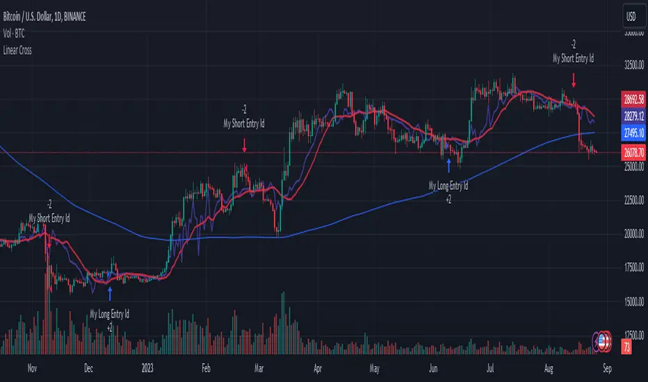
12/26-IT strategyBase of this Strategy is crossover of 12EMA on 26EMA.
Also multiple other criteria has to meet for buy signal, Criterias mentioned below
//////////////////////////////////
There two entry option to select. Either one or both can be selected:
1. Only 12/26 Cross over
a. 12/26 crossover.
b. RSI (14) value to be between a range (RSI is inbuilt, but lower and upper range can be defined in settings)
c. MACD (12, 26) to be positive and above signal line (this is inbuilt)
2. Recent 12/26 Cross over and closing above pivot point(resistance)
a. 12/26 crossover has to be recent, CrossOverLookbackCandles value will look for crossover in # previous candles..
b. RSI (14) value to be between a range (RSI is inbuilt, but lower and upper range can be defined in settings)
c. MACD (12, 26) to be positive and above signal line (this is inbuilt)
d. closing above resistance line
//////////////////////////////////
For Exit we have three options. you can select any SL as per your need, multiple SLs can also be selected
1. Trailing Stop Loss.
Source for TSL is adjustable(open, close, high or low), also you have to mention % below your source TSL has to be placed.
Once closing is below TSL, exit will be triggered.
2. Closing below 7SMA
After 7SMA SL is enabled, 7SMA will be plotted on chart and exit signal will be triggered when closing is below 7SMA.
Choose this option for LESS risk and rewards
3. 12/26 Crossdown
Once 12EMA crossdown below 26EMA, exit will be triggered.
Choose this option for HIGH risk and rewards
//////////////////////////////////
Resistance line is plotted based on left and right candles, if 10(can be changed) is used for both left and right, indicator will look for 10 candles in left and 10 candles in right and if both left and right candle are lower then a line is plotted.
Source has to be selected (close or high)
//////////////////////////////////
Qty mentioned in Buy trigger will be based on BUYVALUE entered
//////////////////////////////////
Multiple Target option is available, if first target is matched how much percentage of qty to be sold can be defined.
If you wish to have only one Target, then exit qty in first target must be 100
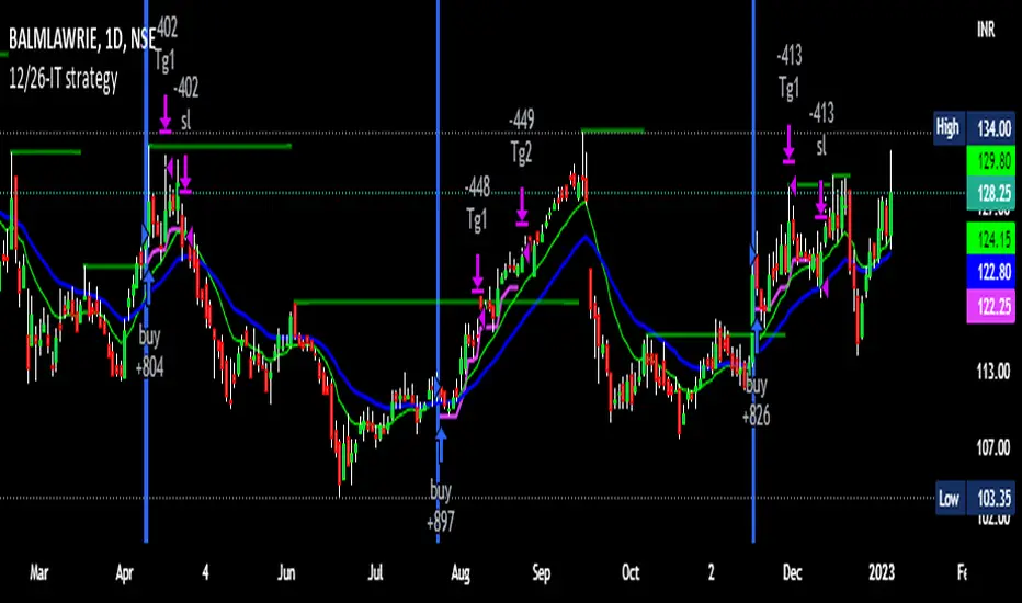
[KBCUSTOM] Histogramified Stochastic RSI The public and regular stoch RSI does not come with a histogram which makes it hard to tell the magnitude of any cross. This version comes with one enabled by default and with includes buy and sell triggers on specified crosses.
Buy & Sell Options:
KB Cross Factor: this is the minimum stochastic change between candles that needs to be exceeded in order to trigger a buy or sell signal. For instance, if the previous candle has a value of -20, and the next one has 10, then the factor should be 30 in order for it to trigger a signal.
KB Cross Threshold: in order to minimize bad signals due to weak trend, you can set the minimum stochastic value any candle should have for an order signal to trigger. For instance, say the stochastic has a good cross factor (i.e. 30) and is met, and the stochastic has a value of 10 but your cross threshold is set at 20, then the signal will not trigger unless it is actually 20 or higher.
Let me know how it works.
Cheers.

Multiple MACD RSI simple strategySimple strategy script I've had for a while but looks like I never published.
Although it is one of my most simple it seems to have the best profitability. It is pretty rough though. the Stoch RSI has only a little weight to the trade trigger. I'll refine it more over time or you can by all means. Basically the Stoch RSI current K line has to be OVER 40 to trigger a SELL. It has no effect on buy side.
The triggers are roughly as follows:
Year - since so many assets have gone 2x, 3x, 10x+ since 2013 having a strategy that earns a 500% return from 2013 to now isn't that good if buy-and-holding would have got you 800%. This eliminates some of that noise and makes it a little easier to quickly gauge success. So buy/sell trigger need a value of greater or equal to 2018 (default)
MACD 1 - First MACD (short) needs to indicate greater than 0 to buy or less than 0 to sell.
MACD 2 - Same as MACD1 but for second MACD set (long)
Uptrend - Latest close + high divided by last periods close + high needs to be grater than 1. So if latest is 34.30 close and 34.60 high and previous interval is 34.80 close and 34.82 high, that is 0.99 and will not trigger a buy trade.
Downtrend - Same thing but close + low and less than 1.
This script/strategy is pretty rough but if there is interest I'll polish it more since it is a pretty solid but simple strategy for most assets.
