Smart Cloud by Ilker (Custom Matriks)A Proprietary Hybrid Trend System for All Major Financial Assets
This indicator, originally developed for the Matriks platform, is a highly effective hybrid trend identification system designed for day-to-day analysis across all major asset classes, including Stocks, Forex, Indices, and Cryptocurrencies. It combines the forward-looking principle of the Ichimoku Kinko Hyo Cloud with heavily smoothed Moving Averages (MAs) to create a clear, visually guided trading signal. (Daily Timeframe recommended for optimal results).
📊 Algorithmic Structure and Parameters
The "Smart Cloud" utilizes six primary user-adjustable parameters that govern its sensitivity and shape, moving away from standard Ichimoku settings to provide a robust, customized trend view:
P1, P2, P3 (60, 56, 248): These long-term settings define the core structure and width of the cloud, acting as the primary dynamic support and resistance zone. The significantly longer P3 (Lagging Period) ensures the cloud reflects strong, deep market cycles.
P4 (Displacement 26): Maintains the traditional Ichimoku principle of projecting the cloud 26 periods forward to provide a predictive view of future trend support/resistance.
P5 (MA50 - Blue) & P6 (MA10 - Purple): These are the two primary Moving Averages plotted inside the cloud. They serve as fast-response momentum lines:
P5 (MA50): Represents the middle-term trend average.
P6 (MA10): Represents the short-term market momentum.
📈 Core Trend and Signal Interpretation
The indicator provides powerful trend identification based on three key components:
The Cloud (Kumo):
Green Cloud (Bullish): Indicates the dominant trend is up, suggesting dynamic support for price action.
Red Cloud (Bearish): Indicates the dominant trend is down, suggesting dynamic resistance.
The thickness and slope of the cloud are key indicators of trend strength.
MA Crossover Signal (Blue/Purple):
Buy Signal: When the faster Purple MA (P6=10) crosses above the slower Blue MA (P5=50).
Sell Signal: When the faster Purple MA (P6=10) crosses below the slower Blue MA (P5=50).
Price Action & Confirmation:
The most powerful signals occur when a MA Crossover is confirmed by price breaking out of the cloud in the same direction.
Price above the cloud and MA crossover to the upside suggests a strong buy entry.
Disclaimer: This tool is intended for analysis and decision-making support. It is not financial advice. Always use stop-loss orders and manage your risk accordingly.
Algotrading

Apex Edge – Wolfe Wave HunterApex Edge – Wolfe Wave Hunter
The modern Wolfe Wave, rebuilt for the algo era
This isn’t just another Wolfe Wave indicator. Classic Wolfe detection is rigid, outdated, and rarely tradable. Apex Edge – Wolfe Wave Hunter re-engineers the pattern into a modern, SMC-driven model that adapts to today’s liquidity-dominated markets. It’s not about drawing pretty shapes – it’s about extracting precision entries with asymmetric risk-to-reward potential.
🔎 What it does
Automatic Wolfe Wave Detection
Identifies bullish and bearish Wolfe Wave structures using pivot-based logic, symmetry filters, and slope tolerances.
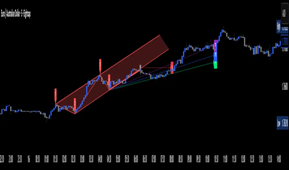
Channel Glow Zones
Highlights the Wolfe channel and projects it forward into the future (bars are user-defined). This allows you to see the full potential of the trade before price even begins its move.
Stop Loss (SL) & Entry Arrow
At the completion of Wave 5, the algo prints a Stop Loss line and a tiny entry arrow (green for bullish, red for bearish). but the colours can be changed in user settings. This is the “execution point” — where the Wolfe setup becomes tradable.
Target Projection Lines
TP1 (EPA): Derived from the traditional 1–4 line projection.
TP2 (1.272 Fib): Optional secondary profit target.
TP3 (1.618 Fib): Optional extended target for large runners.
All TP lines extend into the future, so you can track them as price evolves.
Volume Confirmation (optional)
A relative volume filter ensures Wave 5 is formed with meaningful market participation before a setup is confirmed.
Alerts (ready out of the box)
Custom alerts can be fired whenever a bullish or bearish Wolfe Wave is confirmed. No need to babysit the charts — let the script notify you.
⚙️ Customisation & User Control
Every trader’s market and style is different. That’s why Wolfe Wave Hunter is fully customisable:
Arrow Colours & Size
Works on both light and dark charts. Choose your own bullish/bearish entry arrow colours for maximum visibility.
Tolerance Levels
Adjust symmetry and slope tolerance to refine how strict the channel rules are.
Tighter settings = fewer but cleaner zones.
Looser settings = more frequent setups, but with slightly lower structural quality.
Channel Glow Projection
Define how many bars forward the channel is drawn. This controls how far into the future your Wolfe zones are extended.
Stop Loss Line Length
Keep the SL visible without it extending infinitely across your chart.
Take Profit Line Colors
Each TP projection can be styled to your preference, allowing you to clearly separate TP1, TP2, and TP3.
This isn’t a one-size-fits-all tool. You can shape Wolfe detection logic to match the pairs, timeframes, and market conditions you trade most.
🚀 Why it’s different
Classic Wolfe waves are rare — this script adapts the model into something practical and tradeable in modern markets.
Liquidity-aligned — many setups align with structural sweeps of Wave 3 liquidity before driving into profit.
Entry built-in — most Wolfe scripts only draw the structure. Wolfe Wave Hunter gives you a precise entry point, SL, and projected TPs.
Backtest-friendly — you’ll quickly discover which assets respect Wolfe waves and which don’t, creating your own high-probability Wolfe watchlist.
⚠️ Limitations & Disclaimer
Not all markets respect Wolfe Waves. Some FX pairs, metals, and indices respect the structure beautifully; others do not. Backtest and create your own shortlist.
No guaranteed sweeps. Many entries occur after a liquidity sweep of Wave 3, but not all. The algo is designed to detect Wolfe completion, not enforce textbook liquidity rules.
Probabilistic, not predictive. Wolfe setups don’t win every time. Always use risk management.
High-RR focus. This is not a high-frequency tool. It’s designed for precision, asymmetric setups where risk is small and reward potential is large.
✅ The Bottom Line
Apex Edge – Wolfe Wave Hunter is a modern reimagination of the Wolfe Wave. It blends structural geometry, liquidity dynamics, and algo-driven execution into a single tool that:
Detects the pattern automatically
Provides SL, entry, and TP levels
Offers alerts for hands-off trading
Allows deep customisation for different markets
When it hits, it delivers outstanding risk-to-reward. Backtest, refine your tolerances, and build your watchlist of assets where Wolfe structures consistently pay.
This isn’t just Wolfe detection — it’s Wolfe trading, rebuilt for the modern trader.
Developer Notes - As always with the Apex Edge Brand, user feedback and recommendations will always be respected. Simply drop us a message with your comments and we will endeavour to address your needs in future version updates.
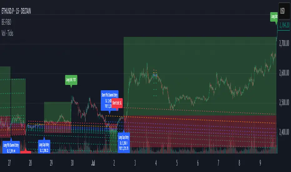
BE-Fib Channel 2 Sided Trading█ Overview:
"BE-Fib Channel 2 Sided Trading" indicator is built with the thought of 2 profound setups named "Cup & Handle (C&H)" and "Fibonacci Channel Trading (FCT)" with the context of "day trading" or with a minimum holding period.
█ Similarities, Day Trading Context & Error Patterns:
While the known fact is that both C&H and FCT provide setups with lesser risk with bigger returns, they both share the similar "Base Pattern".
Note: Inverse of the above Image shall switch the setups between long vs short.
Since the indicator is designed for smaller time-frame candles, there may be instances where the "base pattern" does not visually resemble a Cup & Handle (C&H) pattern. However, patterns are validated using pivot points. The points labeled "A" and "C" can be equal or slightly slanted. Settings of the Indicator allows traders a flexibility to control the angle of these points to spot the strategies according to set conditions. Therefore, understanding the nuances of these patterns is crucial for effective decision-making.
█ 2 Sided Edge: FCT suggests to take trade closer to the yellow line to get better RR ratio. this leaves a small chance of doubt as to; what if price is intended to break the Yellow line thereby activating the C&H.
Wait for the confirmation is a Big FOMO with a compromised RR.
Hence, This indicator is designed to handle both the patterns based on the strength, FIFO and pattern occurring delay.
█ How to Use this Indicator:
Step 1: Enable the Show Sample Sensitivity option to understand the angle of yellow line shown in the sample image. By enabling this option, On the last bar you shall see 4 lines being plotted depicting the max angle which is acceptable for both long and short trades.
Note: Angle can be controlled via setting "Sensitivity".
Higher Sensitivity --> Higher Setup identification --> can lead to failed setups due to 2 sided trading.
Lower Sensitivity --> Lower Setup identification --> can increase the changes of being right.
Step 2: Adjust the look back & look forward periods which shall be used for identifying patterns.
Note: Smaller values can lead to more setups being identified but can hamper the performance of the indicator while increasing the chances of failures. larger values identifies more significant setup but leads to more waiting period thereby compromising on the RR.
Step 3: Adjust the Base Range.
Note: Smaller values can lead to more setups being identified but can hamper the performance of the indicator while increasing the chances of failures. larger values identifies more significant setup but leads to more Risk on play.
Step 4: set the Entry level for FCT & Set the SL for Both FCT & C&H and Target Reward ratio for C&H.
█ Features of Indicator & How it works:
1. Patterns are being identified using Pivot Points method.
2. Tracks & validates both the setups simultaneously on every candle and traded one at a time based on FIFO, New setups found in-between, Defined Entry Levels while on wait for the other pattern to get activated.
3. Alerts added for trade events.
4. FCT setups are generally traded with trailed SL level and increasing Target level on every completed bar. while C&H has the standard SL & TP level with no Trail SL option.
DISCLAIMER: No sharing, copying, reselling, modifying, or any other forms of use are authorized for our documents, script / strategy, and the information published with them. This informational planning script / strategy is strictly for individual use and educational purposes only. This is not financial or investment advice. Investments are always made at your own risk and are based on your personal judgement. I am not responsible for any losses you may incur. Please invest wisely.
Happy to receive suggestions and feedback in order to improve the performance of the indicator better.
PnL Bubble [%] | Fractalyst1. What's the indicator purpose?
The PnL Bubble indicator transforms your strategy's trade PnL percentages into an interactive bubble chart with professional-grade statistics and performance analytics. It helps traders quickly assess system profitability, understand win/loss distribution patterns, identify outliers, and make data-driven strategy improvements.
How does it work?
Think of this indicator as a visual report card for your trading performance. Here's what it does:
What You See
Colorful Bubbles: Each bubble represents one of your trades
Blue/Cyan bubbles = Winning trades (you made money)
Red bubbles = Losing trades (you lost money)
Bigger bubbles = Bigger wins or losses
Smaller bubbles = Smaller wins or losses
How It Organizes Your Trades:
Like a Photo Album: Instead of showing all your trades at once (which would be messy), it shows them in "pages" of 500 trades each:
Page 1: Your first 500 trades
Page 2: Trades 501-1000
Page 3: Trades 1001-1500, etc.
What the Numbers Tell You:
Average Win: How much money you typically make on winning trades
Average Loss: How much money you typically lose on losing trades
Expected Value (EV): Whether your trading system makes money over time
Positive EV = Your system is profitable long-term
Negative EV = Your system loses money long-term
Payoff Ratio (R): How your average win compares to your average loss
R > 1 = Your wins are bigger than your losses
R < 1 = Your losses are bigger than your wins
Why This Matters:
At a Glance: You can instantly see if you're a profitable trader or not
Pattern Recognition: Spot if you have more big wins than big losses
Performance Tracking: Watch how your trading improves over time
Realistic Expectations: Understand what "average" performance looks like for your system
The Cool Visual Effects:
Animation: The bubbles glow and shimmer to make the chart more engaging
Highlighting: Your biggest wins and losses get extra attention with special effects
Tooltips: hover any bubble to see details about that specific trade.
What are the underlying calculations?
The indicator processes trade PnL data using a dual-matrix architecture for optimal performance:
Dual-Matrix System:
• Display Matrix (display_matrix): Bounded to 500 trades for rendering performance
• Statistics Matrix (stats_matrix): Unbounded storage for complete statistical accuracy
Trade Classification & Aggregation:
// Separate wins, losses, and break-even trades
if val > 0.0
pos_sum += val // Sum winning trades
pos_count += 1 // Count winning trades
else if val < 0.0
neg_sum += val // Sum losing trades
neg_count += 1 // Count losing trades
else
zero_count += 1 // Count break-even trades
Statistical Averages:
avg_win = pos_count > 0 ? pos_sum / pos_count : na
avg_loss = neg_count > 0 ? math.abs(neg_sum) / neg_count : na
Win/Loss Rates:
total_obs = pos_count + neg_count + zero_count
win_rate = pos_count / total_obs
loss_rate = neg_count / total_obs
Expected Value (EV):
ev_value = (avg_win × win_rate) - (avg_loss × loss_rate)
Payoff Ratio (R):
R = avg_win ÷ |avg_loss|
Contribution Analysis:
ev_pos_contrib = avg_win × win_rate // Positive EV contribution
ev_neg_contrib = avg_loss × loss_rate // Negative EV contribution
How to integrate with any trading strategy?
Equity Change Tracking Method:
//@version=6
strategy("Your Strategy with Equity Change Export", overlay=true)
float prev_trade_equity = na
float equity_change_pct = na
if barstate.isconfirmed and na(prev_trade_equity)
prev_trade_equity := strategy.equity
trade_just_closed = strategy.closedtrades != strategy.closedtrades
if trade_just_closed and not na(prev_trade_equity)
current_equity = strategy.equity
equity_change_pct := ((current_equity - prev_trade_equity) / prev_trade_equity) * 100
prev_trade_equity := current_equity
else
equity_change_pct := na
plot(equity_change_pct, "Equity Change %", display=display.data_window)
Integration Steps:
1. Add equity tracking code to your strategy
2. Load both strategy and PnL Bubble indicator on the same chart
3. In bubble indicator settings, select your strategy's equity tracking output as data source
4. Configure visualization preferences (colors, effects, page navigation)
How does the pagination system work?
The indicator uses an intelligent pagination system to handle large trade datasets efficiently:
Page Organization:
• Page 1: Trades 1-500 (most recent)
• Page 2: Trades 501-1000
• Page 3: Trades 1001-1500
• Page N: Trades to
Example: With 1,500 trades total (3 pages available):
• User selects Page 1: Shows trades 1-500
• User selects Page 4: Automatically falls back to Page 3 (trades 1001-1500)
5. Understanding the Visual Elements
Bubble Visualization:
• Color Coding: Cyan/blue gradients for wins, red gradients for losses
• Size Mapping: Bubble size proportional to trade magnitude (larger = bigger P&L)
• Priority Rendering: Largest trades displayed first to ensure visibility
• Gradient Effects: Color intensity increases with trade magnitude within each category
Interactive Tooltips:
Each bubble displays quantitative trade information:
tooltip_text = outcome + " | PnL: " + pnl_str +
" Date: " + date_str + " " + time_str +
" Trade #" + str.tostring(trade_number) + " (Page " + str.tostring(active_page) + ")" +
" Rank: " + str.tostring(rank) + " of " + str.tostring(n_display_rows) +
" Percentile: " + str.tostring(percentile, "#.#") + "%" +
" Magnitude: " + str.tostring(magnitude_pct, "#.#") + "%"
Example Tooltip:
Win | PnL: +2.45%
Date: 2024.03.15 14:30
Trade #1,247 (Page 3)
Rank: 5 of 347
Percentile: 98.6%
Magnitude: 85.2%
Reference Lines & Statistics:
• Average Win Line: Horizontal reference showing typical winning trade size
• Average Loss Line: Horizontal reference showing typical losing trade size
• Zero Line: Threshold separating wins from losses
• Statistical Labels: EV, R-Ratio, and contribution analysis displayed on chart
What do the statistical metrics mean?
Expected Value (EV):
Represents the mathematical expectation per trade in percentage terms
EV = (Average Win × Win Rate) - (Average Loss × Loss Rate)
Interpretation:
• EV > 0: Profitable system with positive mathematical expectation
• EV = 0: Break-even system, profitability depends on execution
• EV < 0: Unprofitable system with negative mathematical expectation
Example: EV = +0.34% means you expect +0.34% profit per trade on average
Payoff Ratio (R):
Quantifies the risk-reward relationship of your trading system
R = Average Win ÷ |Average Loss|
Interpretation:
• R > 1.0: Wins are larger than losses on average (favorable risk-reward)
• R = 1.0: Wins and losses are equal in magnitude
• R < 1.0: Losses are larger than wins on average (unfavorable risk-reward)
Example: R = 1.5 means your average win is 50% larger than your average loss
Contribution Analysis (Σ):
Breaks down the components of expected value
Positive Contribution (Σ+) = Average Win × Win Rate
Negative Contribution (Σ-) = Average Loss × Loss Rate
Purpose:
• Shows how much wins contribute to overall expectancy
• Shows how much losses detract from overall expectancy
• Net EV = Σ+ - Σ- (Expected Value per trade)
Example: Σ+: 1.23% means wins contribute +1.23% to expectancy
Example: Σ-: -0.89% means losses drag expectancy by -0.89%
Win/Loss Rates:
Win Rate = Count(Wins) ÷ Total Trades
Loss Rate = Count(Losses) ÷ Total Trades
Shows the probability of winning vs losing trades
Higher win rates don't guarantee profitability if average losses exceed average wins
7. Demo Mode & Synthetic Data Generation
When using built-in sources (close, open, etc.), the indicator generates realistic demo trades for testing:
if isBuiltInSource(source_data)
// Generate random trade outcomes with realistic distribution
u_sign = prand(float(time), float(bar_index))
if u_sign < 0.5
v_push := -1.0 // Loss trade
else
// Skewed distribution favoring smaller wins (realistic)
u_mag = prand(float(time) + 9876.543, float(bar_index) + 321.0)
k = 8.0 // Skewness factor
t = math.pow(u_mag, k)
v_push := 2.5 + t * 8.0 // Win trade
Demo Characteristics:
• Realistic win/loss distribution mimicking actual trading patterns
• Skewed distribution favoring smaller wins over large wins
• Deterministic randomness for consistent demo results
• Includes jitter effects to prevent visual overlap
8. Performance Limitations & Optimizations
Display Constraints:
points_count = 500 // Maximum 500 dots per page for optimal performance
Pine Script v6 Limits:
• Label Count: Maximum 500 labels per indicator
• Line Count: Maximum 100 lines per indicator
• Box Count: Maximum 50 boxes per indicator
• Matrix Size: Efficient memory management with dual-matrix system
Optimization Strategies:
• Pagination System: Handle unlimited trades through 500-trade pages
• Priority Rendering: Largest trades displayed first for maximum visibility
• Dual-Matrix Architecture: Separate display (bounded) from statistics (unbounded)
• Smart Fallback: Automatic page clamping prevents empty displays
Impact & Workarounds:
• Visual Limitation: Only 500 trades visible per page
• Statistical Accuracy: Complete dataset used for all calculations
• Navigation: Use page input to browse through entire trade history
• Performance: Smooth operation even with thousands of trades
9. Statistical Accuracy Guarantees
Data Integrity:
• Complete Dataset: Statistics matrix stores ALL trades without limit
• Proper Aggregation: Separate tracking of wins, losses, and break-even trades
• Mathematical Precision: Pine Script v6's enhanced floating-point calculations
• Dual-Matrix System: Display limitations don't affect statistical accuracy
Calculation Validation:
// Verified formulas match standard trading mathematics
avg_win = pos_sum / pos_count // Standard average calculation
win_rate = pos_count / total_obs // Standard probability calculation
ev_value = (avg_win * win_rate) - (avg_loss * loss_rate) // Standard EV formula
Accuracy Features:
• Mathematical Correctness: Formulas follow established trading statistics
• Data Preservation: Complete dataset maintained for all calculations
• Precision Handling: Proper rounding and boundary condition management
• Real-Time Updates: Statistics recalculated on every new trade
10. Advanced Technical Features
Real-Time Animation Engine:
// Shimmer effects with sine wave modulation
offset = math.sin(shimmer_t + phase) * amp
// Dynamic transparency with organic flicker
new_transp = math.min(flicker_limit, math.max(-flicker_limit, cur_transp + dir * flicker_step))
• Sine Wave Shimmer: Dynamic glowing effects on bubbles
• Organic Flicker: Random transparency variations for natural feel
• Extreme Value Highlighting: Special visual treatment for outliers
• Smooth Animations: Tick-based updates for fluid motion
Magnitude-Based Priority Rendering:
// Sort trades by magnitude for optimal visual hierarchy
sort_indices_by_magnitude(values_mat)
• Largest First: Most important trades always visible
• Intelligent Sorting: Custom bubble sort algorithm for trade prioritization
• Performance Optimized: Efficient sorting for real-time updates
• Visual Hierarchy: Ensures critical trades never get hidden
Professional Tooltip System:
• Quantitative Data: Pure numerical information without interpretative language
• Contextual Ranking: Shows trade position within page dataset
• Percentile Analysis: Performance ranking as percentage
• Magnitude Scaling: Relative size compared to page maximum
• Professional Format: Clean, data-focused presentation
11. Quick Start Guide
Step 1: Add Indicator
• Search for "PnL Bubble | Fractalyst" in TradingView indicators
• Add to your chart (works on any timeframe)
Step 2: Configure Data Source
• Demo Mode: Leave source as "close" to see synthetic trading data
• Strategy Mode: Select your strategy's PnL% output as data source
Step 3: Customize Visualization
• Colors: Set positive (cyan), negative (red), and neutral colors
• Page Navigation: Use "Trade Page" input to browse trade history
• Visual Effects: Built-in shimmer and animation effects are enabled by default
Step 4: Analyze Performance
• Study bubble patterns for win/loss distribution
• Review statistical metrics: EV, R-Ratio, Win Rate
• Use tooltips for detailed trade analysis
• Navigate pages to explore full trade history
Step 5: Optimize Strategy
• Identify outlier trades (largest bubbles)
• Analyze risk-reward profile through R-Ratio
• Monitor Expected Value for system profitability
• Use contribution analysis to understand win/loss impact
12. Why Choose PnL Bubble Indicator?
Unique Advantages:
• Advanced Pagination: Handle unlimited trades with smart fallback system
• Dual-Matrix Architecture: Perfect balance of performance and accuracy
• Professional Statistics: Institution-grade metrics with complete data integrity
• Real-Time Animation: Dynamic visual effects for engaging analysis
• Quantitative Tooltips: Pure numerical data without subjective interpretations
• Priority Rendering: Intelligent magnitude-based display ensures critical trades are always visible
Technical Excellence:
• Built with Pine Script v6 for maximum performance and modern features
• Optimized algorithms for smooth operation with large datasets
• Complete statistical accuracy despite display optimizations
• Professional-grade calculations matching institutional trading analytics
Practical Benefits:
• Instantly identify system profitability through visual patterns
• Spot outlier trades and risk management issues
• Understand true risk-reward profile of your strategies
• Make data-driven decisions for strategy optimization
• Professional presentation suitable for performance reporting
Disclaimer & Risk Considerations:
Important: Historical performance metrics, including positive Expected Value (EV), do not guarantee future trading success. Statistical measures are derived from finite sample data and subject to inherent limitations:
• Sample Bias: Historical data may not represent future market conditions or regime changes
• Ergodicity Assumption: Markets are non-stationary; past statistical relationships may break down
• Survivorship Bias: Strategies showing positive historical EV may fail during different market cycles
• Parameter Instability: Optimal parameters identified in backtesting often degrade in forward testing
• Transaction Cost Evolution: Slippage, spreads, and commission structures change over time
• Behavioral Factors: Live trading introduces psychological elements absent in backtesting
• Black Swan Events: Extreme market events can invalidate statistical assumptions instantaneously

Follow-up Buy / Sell Volume Pressure at Supply / Demand Zones█ Overview:
BE-Volume Footprint & Pressure Candles, is an indicator which is preliminarily designed to analyze the supply and demand patterns based on Rally Base Rally (RBR), Drop Base Drop (DBD), Drop Base Rally (DBR) & Rally Base Drop (RBD) concepts in conjunction to volume pressure. Understanding these concepts are crucial. Let's break down why the "Base" is you Best friend in this context.
Commonness in RBR, DBD, DBR, RBD patterns ?
There is an impulse price movement at first, be it rally (price moving up) or the Drop (price moving down), followed by a period of consolidation which is referred as "BASE" and later with another impulse move of price (Rally or Drop).
Why is the Base Important
1. Market Balance: Base represents a balance between buyers and sellers. This is where decisions are made.
2. Confirmation: It confirms the strength of previous impulse move which has happened.
Base & the Liquidity Play:
Supply & Demand Zone predict the presence of all large orders within the limits of the Base Zone. Price is expected to return to the zone to fill the unfilled orders placed by large players.
For the price to move in the intended direction Liquidity plays the major role. hence indicator aims to help traders in identifying those zones where liquidity exists and the volume pressure helps in confirming that liquidity is making its play.
Bottom pane in the below snapshots is a visual representation of Buyers volume pressure (Green Line & the Green filled area) making the price move upwards vs Sellers volume pressure (Red Line & the Red filled area) making the price move downwards.
Top pane in the below snapshots is a visual representation on the pattern identification (Blue marked zone & the Blue line referred as Liquidity level)
Bullish Pressure On Buy Liquidity:
Bearish Pressure On Sell Liquidity:
█ How It Works:
1. Indicator computes technical & mathematical operations such as ATR, delta of Highs & Lows of the candle and Candle ranges to identify the patterns and marks the liquidity lines accordingly.
2. Indicator then waits for price to return to the liquidity levels and checks if Directional volume pressure to flow-in while the prices hover near the Liquidity zones.
3. Once the Volume pressure is evident, loop in to the ride.
█ When It wont Work:
When there no sufficient Liquidity or sustained Opposite volume pressure, trades are expected to fail.
█ Limitations:
Works only on the scripts which has volume info. Relays on LTF candles to determine intra-bar volumes. Hence, Use on TF greater than 1 min and lesser than 15 min.
█ Indicator Features:
1. StrictEntries: employs' tighter rules (rather most significant setups) on the directional volume pressure applied for the price to move. If unchecked, liberal rules applied on the directional volume pressure leading to more setups being identified.
2. Setup Confirmation period: Indicates Waiting period to analyze the directional volume pressure. Early (lesser wait period) is Risky and Late (longer wait period) is too late for the
ride. Find the quant based on the accuracy of the setup provided in the bottom right table.
3. Algo Enabled with Place Holders:
Indicator is equipped with algo alerts, supported with necessary placeholders to trade any instrument like stock, options etc.
Accepted PlaceHolders (Case Sensitive!!)
1. {{ticker}}-->InstrumentName
2. {{datetime}}-->Date & Time Of Order Placement
3. {{close}}-->LTP Price of Script
4. {{TD}}-->Current Level:
Note: Negative Numbers for Short Setup
5. {{EN}} {{SL}} {{TGT}} {{T1}} {{T2}} --> Trade Levels
6. {{Qty}} {{Qty*x}} --> Qty -> Trade Qty mapped in Settings. Replace x with actual number of your choice for the multiplier
7. {{BS}}-->Based on the Direction of Trade Output shall be with B or S (B == Long Trade & S == Short Trade)
8. {{BUYSELL}}-->Based on the Direction of Trade Output shall be with BUY or SELL (BUY == Long Trade & SELL == Short Trade)
9. {{IBUYSELL}}-->Based on the Direction of Trade Output shall be with BUY or SELL (BUY == SHORT Trade & SELL == LONG Trade)
Dynamic Alerts:
10. { {100R0} }-->Dynamic Place Holder 100 Refers to Strike Difference and Zero refers to ATM
11. { {100R-1} }-->Dynamic Place Holder 100 Refers to Strike Difference and -1 refers to
ATM - 100 strike
12. { {50R2} }-->Dynamic Place Holder 50 Refers to Strike Difference and 2 refers to
ATM + (2 * 50 = 100) strike
13. { {"ddMMyy", 0} }-->Dynamically Picks today date in the specified format.
14. { {"ddMMyy", n} }-->replace n with actual number of your choice to Pick date post today date in the specified format.
15. { {"ddMMyy", "MON"} }-->dynamically pick Monday date (coming Monday, if today is not Monday)
Note. for the 2nd Param-->you can choose to specify either Number OR any letter from =>
16. {{CEPE}} {{ICEPE}} {{CP}} {{ICP}} -> Dynamic Option Side CE or C refers to Calls and PE or P refers to Puts. If "I" is used in PlaceHolder text, On long entries PUTs shall be used
Indicator is equipped with customizable Trade & Risk management settings like multiple Take profit levels, Trailing SL.

Markov Chain [3D] | FractalystWhat exactly is a Markov Chain?
This indicator uses a Markov Chain model to analyze, quantify, and visualize the transitions between market regimes (Bull, Bear, Neutral) on your chart. It dynamically detects these regimes in real-time, calculates transition probabilities, and displays them as animated 3D spheres and arrows, giving traders intuitive insight into current and future market conditions.
How does a Markov Chain work, and how should I read this spheres-and-arrows diagram?
Think of three weather modes: Sunny, Rainy, Cloudy.
Each sphere is one mode. The loop on a sphere means “stay the same next step” (e.g., Sunny again tomorrow).
The arrows leaving a sphere show where things usually go next if they change (e.g., Sunny moving to Cloudy).
Some paths matter more than others. A more prominent loop means the current mode tends to persist. A more prominent outgoing arrow means a change to that destination is the usual next step.
Direction isn’t symmetric: moving Sunny→Cloudy can behave differently than Cloudy→Sunny.
Now relabel the spheres to markets: Bull, Bear, Neutral.
Spheres: market regimes (uptrend, downtrend, range).
Self‑loop: tendency for the current regime to continue on the next bar.
Arrows: the most common next regime if a switch happens.
How to read: Start at the sphere that matches current bar state. If the loop stands out, expect continuation. If one outgoing path stands out, that switch is the typical next step. Opposite directions can differ (Bear→Neutral doesn’t have to match Neutral→Bear).
What states and transitions are shown?
The three market states visualized are:
Bullish (Bull): Upward or strong-market regime.
Bearish (Bear): Downward or weak-market regime.
Neutral: Sideways or range-bound regime.
Bidirectional animated arrows and probability labels show how likely the market is to move from one regime to another (e.g., Bull → Bear or Neutral → Bull).
How does the regime detection system work?
You can use either built-in price returns (based on adaptive Z-score normalization) or supply three custom indicators (such as volume, oscillators, etc.).
Values are statistically normalized (Z-scored) over a configurable lookback period.
The normalized outputs are classified into Bull, Bear, or Neutral zones.
If using three indicators, their regime signals are averaged and smoothed for robustness.
How are transition probabilities calculated?
On every confirmed bar, the algorithm tracks the sequence of detected market states, then builds a rolling window of transitions.
The code maintains a transition count matrix for all regime pairs (e.g., Bull → Bear).
Transition probabilities are extracted for each possible state change using Laplace smoothing for numerical stability, and frequently updated in real-time.
What is unique about the visualization?
3D animated spheres represent each regime and change visually when active.
Animated, bidirectional arrows reveal transition probabilities and allow you to see both dominant and less likely regime flows.
Particles (moving dots) animate along the arrows, enhancing the perception of regime flow direction and speed.
All elements dynamically update with each new price bar, providing a live market map in an intuitive, engaging format.
Can I use custom indicators for regime classification?
Yes! Enable the "Custom Indicators" switch and select any three chart series as inputs. These will be normalized and combined (each with equal weight), broadening the regime classification beyond just price-based movement.
What does the “Lookback Period” control?
Lookback Period (default: 100) sets how much historical data builds the probability matrix. Shorter periods adapt faster to regime changes but may be noisier. Longer periods are more stable but slower to adapt.
How is this different from a Hidden Markov Model (HMM)?
It sets the window for both regime detection and probability calculations. Lower values make the system more reactive, but potentially noisier. Higher values smooth estimates and make the system more robust.
How is this Markov Chain different from a Hidden Markov Model (HMM)?
Markov Chain (as here): All market regimes (Bull, Bear, Neutral) are directly observable on the chart. The transition matrix is built from actual detected regimes, keeping the model simple and interpretable.
Hidden Markov Model: The actual regimes are unobservable ("hidden") and must be inferred from market output or indicator "emissions" using statistical learning algorithms. HMMs are more complex, can capture more subtle structure, but are harder to visualize and require additional machine learning steps for training.
A standard Markov Chain models transitions between observable states using a simple transition matrix, while a Hidden Markov Model assumes the true states are hidden (latent) and must be inferred from observable “emissions” like price or volume data. In practical terms, a Markov Chain is transparent and easier to implement and interpret; an HMM is more expressive but requires statistical inference to estimate hidden states from data.
Markov Chain: states are observable; you directly count or estimate transition probabilities between visible states. This makes it simpler, faster, and easier to validate and tune.
HMM: states are hidden; you only observe emissions generated by those latent states. Learning involves machine learning/statistical algorithms (commonly Baum–Welch/EM for training and Viterbi for decoding) to infer both the transition dynamics and the most likely hidden state sequence from data.
How does the indicator avoid “repainting” or look-ahead bias?
All regime changes and matrix updates happen only on confirmed (closed) bars, so no future data is leaked, ensuring reliable real-time operation.
Are there practical tuning tips?
Tune the Lookback Period for your asset/timeframe: shorter for fast markets, longer for stability.
Use custom indicators if your asset has unique regime drivers.
Watch for rapid changes in transition probabilities as early warning of a possible regime shift.
Who is this indicator for?
Quants and quantitative researchers exploring probabilistic market modeling, especially those interested in regime-switching dynamics and Markov models.
Programmers and system developers who need a probabilistic regime filter for systematic and algorithmic backtesting:
The Markov Chain indicator is ideally suited for programmatic integration via its bias output (1 = Bull, 0 = Neutral, -1 = Bear).
Although the visualization is engaging, the core output is designed for automated, rules-based workflows—not for discretionary/manual trading decisions.
Developers can connect the indicator’s output directly to their Pine Script logic (using input.source()), allowing rapid and robust backtesting of regime-based strategies.
It acts as a plug-and-play regime filter: simply plug the bias output into your entry/exit logic, and you have a scientifically robust, probabilistically-derived signal for filtering, timing, position sizing, or risk regimes.
The MC's output is intentionally "trinary" (1/0/-1), focusing on clear regime states for unambiguous decision-making in code. If you require nuanced, multi-probability or soft-label state vectors, consider expanding the indicator or stacking it with a probability-weighted logic layer in your scripting.
Because it avoids subjectivity, this approach is optimal for systematic quants, algo developers building backtested, repeatable strategies based on probabilistic regime analysis.
What's the mathematical foundation behind this?
The mathematical foundation behind this Markov Chain indicator—and probabilistic regime detection in finance—draws from two principal models: the (standard) Markov Chain and the Hidden Markov Model (HMM).
How to use this indicator programmatically?
The Markov Chain indicator automatically exports a bias value (+1 for Bullish, -1 for Bearish, 0 for Neutral) as a plot visible in the Data Window. This allows you to integrate its regime signal into your own scripts and strategies for backtesting, automation, or live trading.
Step-by-Step Integration with Pine Script (input.source)
Add the Markov Chain indicator to your chart.
This must be done first, since your custom script will "pull" the bias signal from the indicator's plot.
In your strategy, create an input using input.source()
Example:
//@version=5
strategy("MC Bias Strategy Example")
mcBias = input.source(close, "MC Bias Source")
After saving, go to your script’s settings. For the “MC Bias Source” input, select the plot/output of the Markov Chain indicator (typically its bias plot).
Use the bias in your trading logic
Example (long only on Bull, flat otherwise):
if mcBias == 1
strategy.entry("Long", strategy.long)
else
strategy.close("Long")
For more advanced workflows, combine mcBias with additional filters or trailing stops.
How does this work behind-the-scenes?
TradingView’s input.source() lets you use any plot from another indicator as a real-time, “live” data feed in your own script (source).
The selected bias signal is available to your Pine code as a variable, enabling logical decisions based on regime (trend-following, mean-reversion, etc.).
This enables powerful strategy modularity : decouple regime detection from entry/exit logic, allowing fast experimentation without rewriting core signal code.
Integrating 45+ Indicators with Your Markov Chain — How & Why
The Enhanced Custom Indicators Export script exports a massive suite of over 45 technical indicators—ranging from classic momentum (RSI, MACD, Stochastic, etc.) to trend, volume, volatility, and oscillator tools—all pre-calculated, centered/scaled, and available as plots.
// Enhanced Custom Indicators Export - 45 Technical Indicators
// Comprehensive technical analysis suite for advanced market regime detection
//@version=6
indicator('Enhanced Custom Indicators Export | Fractalyst', shorttitle='Enhanced CI Export', overlay=false, scale=scale.right, max_labels_count=500, max_lines_count=500)
// |----- Input Parameters -----| //
momentum_group = "Momentum Indicators"
trend_group = "Trend Indicators"
volume_group = "Volume Indicators"
volatility_group = "Volatility Indicators"
oscillator_group = "Oscillator Indicators"
display_group = "Display Settings"
// Common lengths
length_14 = input.int(14, "Standard Length (14)", minval=1, maxval=100, group=momentum_group)
length_20 = input.int(20, "Medium Length (20)", minval=1, maxval=200, group=trend_group)
length_50 = input.int(50, "Long Length (50)", minval=1, maxval=200, group=trend_group)
// Display options
show_table = input.bool(true, "Show Values Table", group=display_group)
table_size = input.string("Small", "Table Size", options= , group=display_group)
// |----- MOMENTUM INDICATORS (15 indicators) -----| //
// 1. RSI (Relative Strength Index)
rsi_14 = ta.rsi(close, length_14)
rsi_centered = rsi_14 - 50
// 2. Stochastic Oscillator
stoch_k = ta.stoch(close, high, low, length_14)
stoch_d = ta.sma(stoch_k, 3)
stoch_centered = stoch_k - 50
// 3. Williams %R
williams_r = ta.stoch(close, high, low, length_14) - 100
// 4. MACD (Moving Average Convergence Divergence)
= ta.macd(close, 12, 26, 9)
// 5. Momentum (Rate of Change)
momentum = ta.mom(close, length_14)
momentum_pct = (momentum / close ) * 100
// 6. Rate of Change (ROC)
roc = ta.roc(close, length_14)
// 7. Commodity Channel Index (CCI)
cci = ta.cci(close, length_20)
// 8. Money Flow Index (MFI)
mfi = ta.mfi(close, length_14)
mfi_centered = mfi - 50
// 9. Awesome Oscillator (AO)
ao = ta.sma(hl2, 5) - ta.sma(hl2, 34)
// 10. Accelerator Oscillator (AC)
ac = ao - ta.sma(ao, 5)
// 11. Chande Momentum Oscillator (CMO)
cmo = ta.cmo(close, length_14)
// 12. Detrended Price Oscillator (DPO)
dpo = close - ta.sma(close, length_20)
// 13. Price Oscillator (PPO)
ppo = ta.sma(close, 12) - ta.sma(close, 26)
ppo_pct = (ppo / ta.sma(close, 26)) * 100
// 14. TRIX
trix_ema1 = ta.ema(close, length_14)
trix_ema2 = ta.ema(trix_ema1, length_14)
trix_ema3 = ta.ema(trix_ema2, length_14)
trix = ta.roc(trix_ema3, 1) * 10000
// 15. Klinger Oscillator
klinger = ta.ema(volume * (high + low + close) / 3, 34) - ta.ema(volume * (high + low + close) / 3, 55)
// 16. Fisher Transform
fisher_hl2 = 0.5 * (hl2 - ta.lowest(hl2, 10)) / (ta.highest(hl2, 10) - ta.lowest(hl2, 10)) - 0.25
fisher = 0.5 * math.log((1 + fisher_hl2) / (1 - fisher_hl2))
// 17. Stochastic RSI
stoch_rsi = ta.stoch(rsi_14, rsi_14, rsi_14, length_14)
stoch_rsi_centered = stoch_rsi - 50
// 18. Relative Vigor Index (RVI)
rvi_num = ta.swma(close - open)
rvi_den = ta.swma(high - low)
rvi = rvi_den != 0 ? rvi_num / rvi_den : 0
// 19. Balance of Power (BOP)
bop = (close - open) / (high - low)
// |----- TREND INDICATORS (10 indicators) -----| //
// 20. Simple Moving Average Momentum
sma_20 = ta.sma(close, length_20)
sma_momentum = ((close - sma_20) / sma_20) * 100
// 21. Exponential Moving Average Momentum
ema_20 = ta.ema(close, length_20)
ema_momentum = ((close - ema_20) / ema_20) * 100
// 22. Parabolic SAR
sar = ta.sar(0.02, 0.02, 0.2)
sar_trend = close > sar ? 1 : -1
// 23. Linear Regression Slope
lr_slope = ta.linreg(close, length_20, 0) - ta.linreg(close, length_20, 1)
// 24. Moving Average Convergence (MAC)
mac = ta.sma(close, 10) - ta.sma(close, 30)
// 25. Trend Intensity Index (TII)
tii_sum = 0.0
for i = 1 to length_20
tii_sum += close > close ? 1 : 0
tii = (tii_sum / length_20) * 100
// 26. Ichimoku Cloud Components
ichimoku_tenkan = (ta.highest(high, 9) + ta.lowest(low, 9)) / 2
ichimoku_kijun = (ta.highest(high, 26) + ta.lowest(low, 26)) / 2
ichimoku_signal = ichimoku_tenkan > ichimoku_kijun ? 1 : -1
// 27. MESA Adaptive Moving Average (MAMA)
mama_alpha = 2.0 / (length_20 + 1)
mama = ta.ema(close, length_20)
mama_momentum = ((close - mama) / mama) * 100
// 28. Zero Lag Exponential Moving Average (ZLEMA)
zlema_lag = math.round((length_20 - 1) / 2)
zlema_data = close + (close - close )
zlema = ta.ema(zlema_data, length_20)
zlema_momentum = ((close - zlema) / zlema) * 100
// |----- VOLUME INDICATORS (6 indicators) -----| //
// 29. On-Balance Volume (OBV)
obv = ta.obv
// 30. Volume Rate of Change (VROC)
vroc = ta.roc(volume, length_14)
// 31. Price Volume Trend (PVT)
pvt = ta.pvt
// 32. Negative Volume Index (NVI)
nvi = 0.0
nvi := volume < volume ? nvi + ((close - close ) / close ) * nvi : nvi
// 33. Positive Volume Index (PVI)
pvi = 0.0
pvi := volume > volume ? pvi + ((close - close ) / close ) * pvi : pvi
// 34. Volume Oscillator
vol_osc = ta.sma(volume, 5) - ta.sma(volume, 10)
// 35. Ease of Movement (EOM)
eom_distance = high - low
eom_box_height = volume / 1000000
eom = eom_box_height != 0 ? eom_distance / eom_box_height : 0
eom_sma = ta.sma(eom, length_14)
// 36. Force Index
force_index = volume * (close - close )
force_index_sma = ta.sma(force_index, length_14)
// |----- VOLATILITY INDICATORS (10 indicators) -----| //
// 37. Average True Range (ATR)
atr = ta.atr(length_14)
atr_pct = (atr / close) * 100
// 38. Bollinger Bands Position
bb_basis = ta.sma(close, length_20)
bb_dev = 2.0 * ta.stdev(close, length_20)
bb_upper = bb_basis + bb_dev
bb_lower = bb_basis - bb_dev
bb_position = bb_dev != 0 ? (close - bb_basis) / bb_dev : 0
bb_width = bb_dev != 0 ? (bb_upper - bb_lower) / bb_basis * 100 : 0
// 39. Keltner Channels Position
kc_basis = ta.ema(close, length_20)
kc_range = ta.ema(ta.tr, length_20)
kc_upper = kc_basis + (2.0 * kc_range)
kc_lower = kc_basis - (2.0 * kc_range)
kc_position = kc_range != 0 ? (close - kc_basis) / kc_range : 0
// 40. Donchian Channels Position
dc_upper = ta.highest(high, length_20)
dc_lower = ta.lowest(low, length_20)
dc_basis = (dc_upper + dc_lower) / 2
dc_position = (dc_upper - dc_lower) != 0 ? (close - dc_basis) / (dc_upper - dc_lower) : 0
// 41. Standard Deviation
std_dev = ta.stdev(close, length_20)
std_dev_pct = (std_dev / close) * 100
// 42. Relative Volatility Index (RVI)
rvi_up = ta.stdev(close > close ? close : 0, length_14)
rvi_down = ta.stdev(close < close ? close : 0, length_14)
rvi_total = rvi_up + rvi_down
rvi_volatility = rvi_total != 0 ? (rvi_up / rvi_total) * 100 : 50
// 43. Historical Volatility
hv_returns = math.log(close / close )
hv = ta.stdev(hv_returns, length_20) * math.sqrt(252) * 100
// 44. Garman-Klass Volatility
gk_vol = math.log(high/low) * math.log(high/low) - (2*math.log(2)-1) * math.log(close/open) * math.log(close/open)
gk_volatility = math.sqrt(ta.sma(gk_vol, length_20)) * 100
// 45. Parkinson Volatility
park_vol = math.log(high/low) * math.log(high/low)
parkinson = math.sqrt(ta.sma(park_vol, length_20) / (4 * math.log(2))) * 100
// 46. Rogers-Satchell Volatility
rs_vol = math.log(high/close) * math.log(high/open) + math.log(low/close) * math.log(low/open)
rogers_satchell = math.sqrt(ta.sma(rs_vol, length_20)) * 100
// |----- OSCILLATOR INDICATORS (5 indicators) -----| //
// 47. Elder Ray Index
elder_bull = high - ta.ema(close, 13)
elder_bear = low - ta.ema(close, 13)
elder_power = elder_bull + elder_bear
// 48. Schaff Trend Cycle (STC)
stc_macd = ta.ema(close, 23) - ta.ema(close, 50)
stc_k = ta.stoch(stc_macd, stc_macd, stc_macd, 10)
stc_d = ta.ema(stc_k, 3)
stc = ta.stoch(stc_d, stc_d, stc_d, 10)
// 49. Coppock Curve
coppock_roc1 = ta.roc(close, 14)
coppock_roc2 = ta.roc(close, 11)
coppock = ta.wma(coppock_roc1 + coppock_roc2, 10)
// 50. Know Sure Thing (KST)
kst_roc1 = ta.roc(close, 10)
kst_roc2 = ta.roc(close, 15)
kst_roc3 = ta.roc(close, 20)
kst_roc4 = ta.roc(close, 30)
kst = ta.sma(kst_roc1, 10) + 2*ta.sma(kst_roc2, 10) + 3*ta.sma(kst_roc3, 10) + 4*ta.sma(kst_roc4, 15)
// 51. Percentage Price Oscillator (PPO)
ppo_line = ((ta.ema(close, 12) - ta.ema(close, 26)) / ta.ema(close, 26)) * 100
ppo_signal = ta.ema(ppo_line, 9)
ppo_histogram = ppo_line - ppo_signal
// |----- PLOT MAIN INDICATORS -----| //
// Plot key momentum indicators
plot(rsi_centered, title="01_RSI_Centered", color=color.purple, linewidth=1)
plot(stoch_centered, title="02_Stoch_Centered", color=color.blue, linewidth=1)
plot(williams_r, title="03_Williams_R", color=color.red, linewidth=1)
plot(macd_histogram, title="04_MACD_Histogram", color=color.orange, linewidth=1)
plot(cci, title="05_CCI", color=color.green, linewidth=1)
// Plot trend indicators
plot(sma_momentum, title="06_SMA_Momentum", color=color.navy, linewidth=1)
plot(ema_momentum, title="07_EMA_Momentum", color=color.maroon, linewidth=1)
plot(sar_trend, title="08_SAR_Trend", color=color.teal, linewidth=1)
plot(lr_slope, title="09_LR_Slope", color=color.lime, linewidth=1)
plot(mac, title="10_MAC", color=color.fuchsia, linewidth=1)
// Plot volatility indicators
plot(atr_pct, title="11_ATR_Pct", color=color.yellow, linewidth=1)
plot(bb_position, title="12_BB_Position", color=color.aqua, linewidth=1)
plot(kc_position, title="13_KC_Position", color=color.olive, linewidth=1)
plot(std_dev_pct, title="14_StdDev_Pct", color=color.silver, linewidth=1)
plot(bb_width, title="15_BB_Width", color=color.gray, linewidth=1)
// Plot volume indicators
plot(vroc, title="16_VROC", color=color.blue, linewidth=1)
plot(eom_sma, title="17_EOM", color=color.red, linewidth=1)
plot(vol_osc, title="18_Vol_Osc", color=color.green, linewidth=1)
plot(force_index_sma, title="19_Force_Index", color=color.orange, linewidth=1)
plot(obv, title="20_OBV", color=color.purple, linewidth=1)
// Plot additional oscillators
plot(ao, title="21_Awesome_Osc", color=color.navy, linewidth=1)
plot(cmo, title="22_CMO", color=color.maroon, linewidth=1)
plot(dpo, title="23_DPO", color=color.teal, linewidth=1)
plot(trix, title="24_TRIX", color=color.lime, linewidth=1)
plot(fisher, title="25_Fisher", color=color.fuchsia, linewidth=1)
// Plot more momentum indicators
plot(mfi_centered, title="26_MFI_Centered", color=color.yellow, linewidth=1)
plot(ac, title="27_AC", color=color.aqua, linewidth=1)
plot(ppo_pct, title="28_PPO_Pct", color=color.olive, linewidth=1)
plot(stoch_rsi_centered, title="29_StochRSI_Centered", color=color.silver, linewidth=1)
plot(klinger, title="30_Klinger", color=color.gray, linewidth=1)
// Plot trend continuation
plot(tii, title="31_TII", color=color.blue, linewidth=1)
plot(ichimoku_signal, title="32_Ichimoku_Signal", color=color.red, linewidth=1)
plot(mama_momentum, title="33_MAMA_Momentum", color=color.green, linewidth=1)
plot(zlema_momentum, title="34_ZLEMA_Momentum", color=color.orange, linewidth=1)
plot(bop, title="35_BOP", color=color.purple, linewidth=1)
// Plot volume continuation
plot(nvi, title="36_NVI", color=color.navy, linewidth=1)
plot(pvi, title="37_PVI", color=color.maroon, linewidth=1)
plot(momentum_pct, title="38_Momentum_Pct", color=color.teal, linewidth=1)
plot(roc, title="39_ROC", color=color.lime, linewidth=1)
plot(rvi, title="40_RVI", color=color.fuchsia, linewidth=1)
// Plot volatility continuation
plot(dc_position, title="41_DC_Position", color=color.yellow, linewidth=1)
plot(rvi_volatility, title="42_RVI_Volatility", color=color.aqua, linewidth=1)
plot(hv, title="43_Historical_Vol", color=color.olive, linewidth=1)
plot(gk_volatility, title="44_GK_Volatility", color=color.silver, linewidth=1)
plot(parkinson, title="45_Parkinson_Vol", color=color.gray, linewidth=1)
// Plot final oscillators
plot(rogers_satchell, title="46_RS_Volatility", color=color.blue, linewidth=1)
plot(elder_power, title="47_Elder_Power", color=color.red, linewidth=1)
plot(stc, title="48_STC", color=color.green, linewidth=1)
plot(coppock, title="49_Coppock", color=color.orange, linewidth=1)
plot(kst, title="50_KST", color=color.purple, linewidth=1)
// Plot final indicators
plot(ppo_histogram, title="51_PPO_Histogram", color=color.navy, linewidth=1)
plot(pvt, title="52_PVT", color=color.maroon, linewidth=1)
// |----- Reference Lines -----| //
hline(0, "Zero Line", color=color.gray, linestyle=hline.style_dashed, linewidth=1)
hline(50, "Midline", color=color.gray, linestyle=hline.style_dotted, linewidth=1)
hline(-50, "Lower Midline", color=color.gray, linestyle=hline.style_dotted, linewidth=1)
hline(25, "Upper Threshold", color=color.gray, linestyle=hline.style_dotted, linewidth=1)
hline(-25, "Lower Threshold", color=color.gray, linestyle=hline.style_dotted, linewidth=1)
// |----- Enhanced Information Table -----| //
if show_table and barstate.islast
table_position = position.top_right
table_text_size = table_size == "Tiny" ? size.tiny : table_size == "Small" ? size.small : size.normal
var table info_table = table.new(table_position, 3, 18, bgcolor=color.new(color.white, 85), border_width=1, border_color=color.gray)
// Headers
table.cell(info_table, 0, 0, 'Category', text_color=color.black, text_size=table_text_size, bgcolor=color.new(color.blue, 70))
table.cell(info_table, 1, 0, 'Indicator', text_color=color.black, text_size=table_text_size, bgcolor=color.new(color.blue, 70))
table.cell(info_table, 2, 0, 'Value', text_color=color.black, text_size=table_text_size, bgcolor=color.new(color.blue, 70))
// Key Momentum Indicators
table.cell(info_table, 0, 1, 'MOMENTUM', text_color=color.purple, text_size=table_text_size, bgcolor=color.new(color.purple, 90))
table.cell(info_table, 1, 1, 'RSI Centered', text_color=color.purple, text_size=table_text_size)
table.cell(info_table, 2, 1, str.tostring(rsi_centered, '0.00'), text_color=color.purple, text_size=table_text_size)
table.cell(info_table, 0, 2, '', text_color=color.blue, text_size=table_text_size)
table.cell(info_table, 1, 2, 'Stoch Centered', text_color=color.blue, text_size=table_text_size)
table.cell(info_table, 2, 2, str.tostring(stoch_centered, '0.00'), text_color=color.blue, text_size=table_text_size)
table.cell(info_table, 0, 3, '', text_color=color.red, text_size=table_text_size)
table.cell(info_table, 1, 3, 'Williams %R', text_color=color.red, text_size=table_text_size)
table.cell(info_table, 2, 3, str.tostring(williams_r, '0.00'), text_color=color.red, text_size=table_text_size)
table.cell(info_table, 0, 4, '', text_color=color.orange, text_size=table_text_size)
table.cell(info_table, 1, 4, 'MACD Histogram', text_color=color.orange, text_size=table_text_size)
table.cell(info_table, 2, 4, str.tostring(macd_histogram, '0.000'), text_color=color.orange, text_size=table_text_size)
table.cell(info_table, 0, 5, '', text_color=color.green, text_size=table_text_size)
table.cell(info_table, 1, 5, 'CCI', text_color=color.green, text_size=table_text_size)
table.cell(info_table, 2, 5, str.tostring(cci, '0.00'), text_color=color.green, text_size=table_text_size)
// Key Trend Indicators
table.cell(info_table, 0, 6, 'TREND', text_color=color.navy, text_size=table_text_size, bgcolor=color.new(color.navy, 90))
table.cell(info_table, 1, 6, 'SMA Momentum %', text_color=color.navy, text_size=table_text_size)
table.cell(info_table, 2, 6, str.tostring(sma_momentum, '0.00'), text_color=color.navy, text_size=table_text_size)
table.cell(info_table, 0, 7, '', text_color=color.maroon, text_size=table_text_size)
table.cell(info_table, 1, 7, 'EMA Momentum %', text_color=color.maroon, text_size=table_text_size)
table.cell(info_table, 2, 7, str.tostring(ema_momentum, '0.00'), text_color=color.maroon, text_size=table_text_size)
table.cell(info_table, 0, 8, '', text_color=color.teal, text_size=table_text_size)
table.cell(info_table, 1, 8, 'SAR Trend', text_color=color.teal, text_size=table_text_size)
table.cell(info_table, 2, 8, str.tostring(sar_trend, '0'), text_color=color.teal, text_size=table_text_size)
table.cell(info_table, 0, 9, '', text_color=color.lime, text_size=table_text_size)
table.cell(info_table, 1, 9, 'Linear Regression', text_color=color.lime, text_size=table_text_size)
table.cell(info_table, 2, 9, str.tostring(lr_slope, '0.000'), text_color=color.lime, text_size=table_text_size)
// Key Volatility Indicators
table.cell(info_table, 0, 10, 'VOLATILITY', text_color=color.yellow, text_size=table_text_size, bgcolor=color.new(color.yellow, 90))
table.cell(info_table, 1, 10, 'ATR %', text_color=color.yellow, text_size=table_text_size)
table.cell(info_table, 2, 10, str.tostring(atr_pct, '0.00'), text_color=color.yellow, text_size=table_text_size)
table.cell(info_table, 0, 11, '', text_color=color.aqua, text_size=table_text_size)
table.cell(info_table, 1, 11, 'BB Position', text_color=color.aqua, text_size=table_text_size)
table.cell(info_table, 2, 11, str.tostring(bb_position, '0.00'), text_color=color.aqua, text_size=table_text_size)
table.cell(info_table, 0, 12, '', text_color=color.olive, text_size=table_text_size)
table.cell(info_table, 1, 12, 'KC Position', text_color=color.olive, text_size=table_text_size)
table.cell(info_table, 2, 12, str.tostring(kc_position, '0.00'), text_color=color.olive, text_size=table_text_size)
// Key Volume Indicators
table.cell(info_table, 0, 13, 'VOLUME', text_color=color.blue, text_size=table_text_size, bgcolor=color.new(color.blue, 90))
table.cell(info_table, 1, 13, 'Volume ROC', text_color=color.blue, text_size=table_text_size)
table.cell(info_table, 2, 13, str.tostring(vroc, '0.00'), text_color=color.blue, text_size=table_text_size)
table.cell(info_table, 0, 14, '', text_color=color.red, text_size=table_text_size)
table.cell(info_table, 1, 14, 'EOM', text_color=color.red, text_size=table_text_size)
table.cell(info_table, 2, 14, str.tostring(eom_sma, '0.000'), text_color=color.red, text_size=table_text_size)
// Key Oscillators
table.cell(info_table, 0, 15, 'OSCILLATORS', text_color=color.purple, text_size=table_text_size, bgcolor=color.new(color.purple, 90))
table.cell(info_table, 1, 15, 'Awesome Osc', text_color=color.blue, text_size=table_text_size)
table.cell(info_table, 2, 15, str.tostring(ao, '0.000'), text_color=color.blue, text_size=table_text_size)
table.cell(info_table, 0, 16, '', text_color=color.red, text_size=table_text_size)
table.cell(info_table, 1, 16, 'Fisher Transform', text_color=color.red, text_size=table_text_size)
table.cell(info_table, 2, 16, str.tostring(fisher, '0.000'), text_color=color.red, text_size=table_text_size)
// Summary Statistics
table.cell(info_table, 0, 17, 'SUMMARY', text_color=color.black, text_size=table_text_size, bgcolor=color.new(color.gray, 70))
table.cell(info_table, 1, 17, 'Total Indicators: 52', text_color=color.black, text_size=table_text_size)
regime_color = rsi_centered > 10 ? color.green : rsi_centered < -10 ? color.red : color.gray
regime_text = rsi_centered > 10 ? "BULLISH" : rsi_centered < -10 ? "BEARISH" : "NEUTRAL"
table.cell(info_table, 2, 17, regime_text, text_color=regime_color, text_size=table_text_size)
This makes it the perfect “indicator backbone” for quantitative and systematic traders who want to prototype, combine, and test new regime detection models—especially in combination with the Markov Chain indicator.
How to use this script with the Markov Chain for research and backtesting:
Add the Enhanced Indicator Export to your chart.
Every calculated indicator is available as an individual data stream.
Connect the indicator(s) you want as custom input(s) to the Markov Chain’s “Custom Indicators” option.
In the Markov Chain indicator’s settings, turn ON the custom indicator mode.
For each of the three custom indicator inputs, select the exported plot from the Enhanced Export script—the menu lists all 45+ signals by name.
This creates a powerful, modular regime-detection engine where you can mix-and-match momentum, trend, volume, or custom combinations for advanced filtering.
Backtest regime logic directly.
Once you’ve connected your chosen indicators, the Markov Chain script performs regime detection (Bull/Neutral/Bear) based on your selected features—not just price returns.
The regime detection is robust, automatically normalized (using Z-score), and outputs bias (1, -1, 0) for plug-and-play integration.
Export the regime bias for programmatic use.
As described above, use input.source() in your Pine Script strategy or system and link the bias output.
You can now filter signals, control trade direction/size, or design pairs-trading that respect true, indicator-driven market regimes.
With this framework, you’re not limited to static or simplistic regime filters. You can rigorously define, test, and refine what “market regime” means for your strategies—using the technical features that matter most to you.
Optimize your signal generation by backtesting across a universe of meaningful indicator blends.
Enhance risk management with objective, real-time regime boundaries.
Accelerate your research: iterate quickly, swap indicator components, and see results with minimal code changes.
Automate multi-asset or pairs-trading by integrating regime context directly into strategy logic.
Add both scripts to your chart, connect your preferred features, and start investigating your best regime-based trades—entirely within the TradingView ecosystem.
References & Further Reading
Ang, A., & Bekaert, G. (2002). “Regime Switches in Interest Rates.” Journal of Business & Economic Statistics, 20(2), 163–182.
Hamilton, J. D. (1989). “A New Approach to the Economic Analysis of Nonstationary Time Series and the Business Cycle.” Econometrica, 57(2), 357–384.
Markov, A. A. (1906). "Extension of the Limit Theorems of Probability Theory to a Sum of Variables Connected in a Chain." The Notes of the Imperial Academy of Sciences of St. Petersburg.
Guidolin, M., & Timmermann, A. (2007). “Asset Allocation under Multivariate Regime Switching.” Journal of Economic Dynamics and Control, 31(11), 3503–3544.
Murphy, J. J. (1999). Technical Analysis of the Financial Markets. New York Institute of Finance.
Brock, W., Lakonishok, J., & LeBaron, B. (1992). “Simple Technical Trading Rules and the Stochastic Properties of Stock Returns.” Journal of Finance, 47(5), 1731–1764.
Zucchini, W., MacDonald, I. L., & Langrock, R. (2017). Hidden Markov Models for Time Series: An Introduction Using R (2nd ed.). Chapman and Hall/CRC.
On Quantitative Finance and Markov Models:
Lo, A. W., & Hasanhodzic, J. (2009). The Heretics of Finance: Conversations with Leading Practitioners of Technical Analysis. Bloomberg Press.
Patterson, S. (2016). The Man Who Solved the Market: How Jim Simons Launched the Quant Revolution. Penguin Press.
TradingView Pine Script Documentation: www.tradingview.com
TradingView Blog: “Use an Input From Another Indicator With Your Strategy” www.tradingview.com
GeeksforGeeks: “What is the Difference Between Markov Chains and Hidden Markov Models?” www.geeksforgeeks.org
What makes this indicator original and unique?
- On‑chart, real‑time Markov. The chain is drawn directly on your chart. You see the current regime, its tendency to stay (self‑loop), and the usual next step (arrows) as bars confirm.
- Source‑agnostic by design. The engine runs on any series you select via input.source() — price, your own oscillator, a composite score, anything you compute in the script.
- Automatic normalization + regime mapping. Different inputs live on different scales. The script standardizes your chosen source and maps it into clear regimes (e.g., Bull / Bear / Neutral) without you micromanaging thresholds each time.
- Rolling, bar‑by‑bar learning. Transition tendencies are computed from a rolling window of confirmed bars. What you see is exactly what the market did in that window.
- Fast experimentation. Switch the source, adjust the window, and the Markov view updates instantly. It’s a rapid way to test ideas and feel regime persistence/switch behavior.
Integrate your own signals (using input.source())
- In settings, choose the Source . This is powered by input.source() .
- Feed it price, an indicator you compute inside the script, or a custom composite series.
- The script will automatically normalize that series and process it through the Markov engine, mapping it to regimes and updating the on‑chart spheres/arrows in real time.
Credits:
Deep gratitude to @RicardoSantos for both the foundational Markov chain processing engine and inspiring open-source contributions, which made advanced probabilistic market modeling accessible to the TradingView community.
Special thanks to @Alien_Algorithms for the innovative and visually stunning 3D sphere logic that powers the indicator’s animated, regime-based visualization.
Disclaimer
This tool summarizes recent behavior. It is not financial advice and not a guarantee of future results.

Order Blocks v2Order Blocks v2 – Smart OB Detection with Time & FVG Filters
Order Blocks v2 is an advanced tool designed to identify potential institutional footprints in the market by dynamically plotting bullish and bearish order blocks.
This indicator refines classic OB logic by combining:
Fractal-based break conditions
Time-level filtering (Power of 3)
Optional Fair Value Gap (FVG) confirmation
Real-time plotting and auto-invalidation
Perfect for traders using ICT, Smart Money, or algorithmic timing models like Hopplipka.
🧠 What the indicator does
Detects order blocks after break of bullish/bearish fractals
Supports 3-bar or 5-bar fractal structures
Allows OB detection based on close breaks or high/low breaks
Optionally confirms OBs only if followed by a Fair Value Gap within N candles
Filters OBs based on specific time levels (3, 7, 11, 14) — core anchors in many algorithmic models
Automatically deletes invalidated OBs once price closes through the zone
⚙️ How it works
The indicator:
Tracks local fractal highs/lows
Once a fractal is broken by price, it backtracks to identify the best OB candle (highest bullish or lowest bearish)
Validates the level by checking:
OB type logic (close or HL break)
Time stamp match with algorithmic time anchors (e.g. 3, 7, 11, 14 – known from the Power of 3 concept)
Optional FVG confirmation after OB
Plots OB zones as lines (body or wick-based) and removes them if invalidated by a candle close
This ensures traders see only valid, active levels — removing noise from broken or out-of-context zones.
🔧 Customization
Choose 3-bar or 5-bar fractals
OB detection type: close break or HL break
Enable/disable OBs only on times 3, 7, 11, 14 (Hopplipka style)
Optional: require nearby FVG for validation
Line style: solid, dashed, or dotted
Adjust OB length, width, color, and use body or wick for OB height
🚀 How to use it
Add the script to your chart
Choose your preferred OB detection mode and filters
Use plotted OB zones to:
Anticipate price rejections and reversals
Validate Smart Money or ICT-based entry zones
Align setups with algorithmic time sequences (3, 7, 11, 14)
Filter out invalid OBs automatically, keeping your chart clean
The tool is useful on any timeframe but performs best when combined with a liquidity-based or time-anchored trading model.
💡 What makes it original
Combines fractal logic with OB confirmation and time anchors
Implements time-based filtering inspired by Hopplipka’s interpretation of the "Power of 3"
Allows OB validation via optional FVG follow-up — rarely available in public indicators
Auto-cleans invalidated OBs to reduce clutter
Designed to reflect market structure logic used by institutions and algorithms
💬 Why it’s worth using
Order Blocks v2 simplifies one of the most nuanced parts of SMC: identifying clean and high-probability OBs.
It removes subjectivity, adds clear timing logic, and integrates optional confluence tools — like FVG.
For traders serious about algorithmic-level structure and clean setups, this tool delivers both logic and clarity.
⚠️ Important
This indicator:
Is not a signal generator or financial advice tool
Is intended for experienced traders using OB/SMC/time-based logic
Does not predict market direction — it provides visual structural levels only
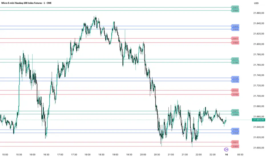
PriceLevels GBGoldbach Price Levels – Identify Algorithmic Key Zones
This open-source indicator is designed to help traders identify potential algorithmic key zones by highlighting price levels ending with specific numbers such as 03, 11, 29, 35, 65, and 71. These levels may act as inflection points or hesitation areas based on observed behavioral patterns in price movement.
What It Does:
📌 Scans and plots horizontal price levels where the price ends with one of the selected number combinations
🎯 Toggle on/off visibility for each number ending
🎨 Customize color and thickness for each level
🏷️ Shows price labels at the end of each line
🌗 Label styles (color/transparency) are adjustable for both dark and light chart themes
🧠 Why Use It:
This tool is ideal for discretionary traders who study market structure through static price anchors. It provides a visual reference for recurring numerical levels that may be used in algorithmic trading models or serve as psychological price zones.
⚠️ Disclaimer:
This script is open-source and intended for educational and analytical purposes only. No trading signals or performance guarantees are provided. Please use your own judgment when applying this tool in a trading context.
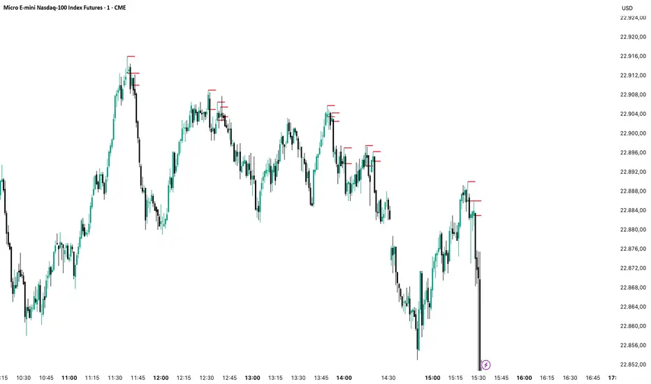
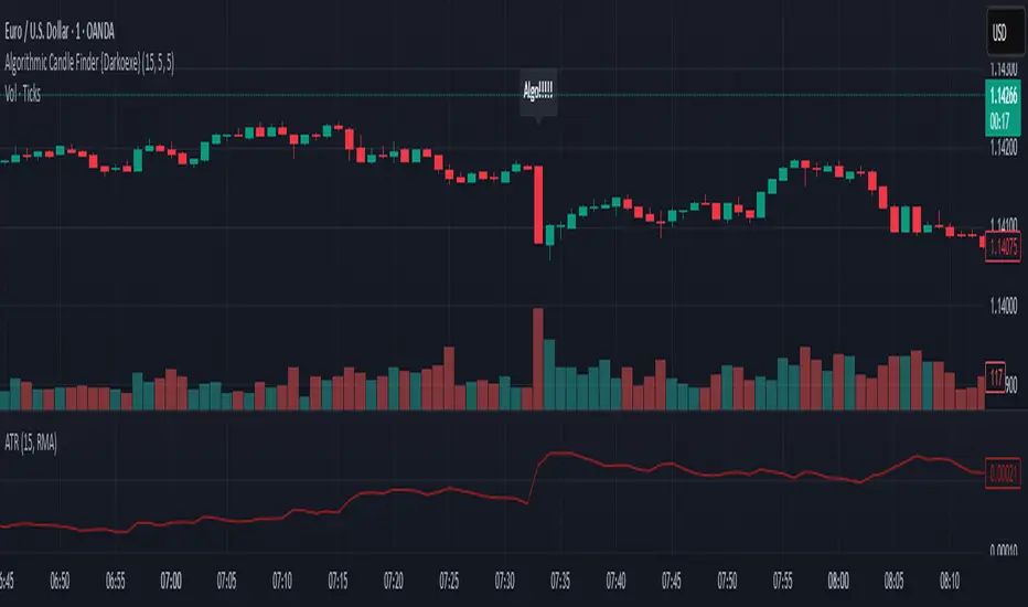
Algorithmic Candle Finder {Darkoexe}Algorithmic Candle Finder Indicator
Algorithmic candles are candles whose size and direction are significantly influenced by institutions or large players using market algorithms. These entities can move large amounts of capital in or out of the market, creating price moves that are often difficult for retail traders to predict or react to.
This can make short-term retail trading risky and inconsistent, especially when unaware of such institutional activity. The goal of this indicator is to help identify such candles, allowing traders to avoid trading during times of potential algorithmic influence.
Detection Criteria:
A candle is marked as algorithmic if either of the following conditions are met:
Size-Based Detection: If the current candle’s size exceeds the Average True Range (ATR) of the previous candle multiplied by the ATR factor input.
Volume-Based Detection: If the current candle’s volume exceeds the average volume of recent candles (e.g., last N candles) multiplied by the volume factor input.
When a candle is deemed algorithmic, a label saying "Algo!!!!!" will appear on the chart above the candle where the condition occurred.
Usage:
Use this indicator to study which times of day algorithmic candles frequently appear. This can help you adjust your strategy to avoid trading during these unpredictable moments.
Analogy:
Think of the market like the game Agar.io: small players (retail traders) collect small pellets to grow, while larger players (institutions) devour smaller ones. The small players must avoid the big ones to survive. Likewise, in trading, retail traders should aim to avoid high-impact algorithmic activity that could “consume” their trades.
Cumulative Intraday Volume with Long/Short LabelsThis indicator calculates a running total of volume for each trading day, then shows on the price chart when that total crosses levels you choose. Every day at 6:00 PM Eastern Time, the total goes back to zero so it always reflects only the current day’s activity. From that moment on, each time a new candle appears the indicator looks at whether the candle closed higher than it opened or lower. If it closed higher, the candle’s volume is added to the running total; if it closed lower, the same volume amount is subtracted. As a result, the total becomes positive when buyers have dominated so far today and negative when sellers have dominated.
Because futures markets close at 6 PM ET, the running total resets exactly then, mirroring the way most intraday traders think in terms of a single session. Throughout the day, you will see this running total move up or down according to whether more volume is happening on green or red candles. Once the total goes above a number you specify (for example, one hundred thousand contracts), the indicator will place a small “Long” label at that candle on the main price chart to let you know buying pressure has reached that level. Similarly, once the total goes below a negative number you choose (for example, minus one hundred thousand), a “Short” label will appear at that candle to signal that selling pressure has reached your chosen threshold. You can set these threshold numbers to whatever makes sense for your trading style or the market you follow.
Because raw volume alone never turns negative, this design uses candle direction as a sign. Green candles (where the close is higher than the open) add volume, and red candles (where the close is lower than the open) subtract volume. Summing those signed volume values tells you in a single number whether buying or selling has been stronger so far today. That number resets every evening, so it does not carry over any buying or selling from previous sessions.
Once you have this indicator on your chart, you simply watch the “summed volume” line as it moves throughout the day. If it climbs past your long threshold, you know buyers are firmly in control and a long entry might make sense. If it falls past your short threshold, you know sellers are firmly in control and a short entry might make sense. In quieter markets or times of low volume, you might use a smaller threshold so that even modest buying or selling pressure will trigger a label. During very active periods, a larger threshold will prevent too many signals when volume spikes frequently.
This approach is straightforward but can be surprisingly powerful. It does not rely on complex formulas or hidden statistical measures. Instead, it simply adds and subtracts daily volume based on candle color, then alerts you when that total reaches levels you care about. Over several years of historical testing, this formula has shown an ability to highlight moments when intraday sentiment shifts decisively from buyers to sellers or vice versa. Because the indicator resets every day at 6 PM, it always reflects only today’s sentiment and remains easy to interpret without carrying over past data. You can use it on any intraday timeframe, but it works especially well on five-minute or fifteen-minute charts for futures contracts.
If you want a clear gauge of whether buyers or sellers are dominating in real time, and you prefer a rule-based method rather than a complex model, this indicator gives you exactly that. It shows net buying or selling pressure at a glance, resets each session like most intraday traders do, and marks the moments when that pressure crosses the levels you decide are important. By combining a daily reset with signed volume, you get a single number that tells you precisely what the crowd is doing at any given moment, without any of the guesswork or hidden calculations that more complicated indicators often carry.

RSI Classic calculationClassic RSI with Moving Average
This script implements the Classic RSI (Relative Strength Index) method with the option to use either an Exponential Moving Average (EMA) or a Simple Moving Average (SMA) for smoothing the gains and losses. This custom implementation primarily aims to resolve a specific issue I encountered when cross-referencing RSI values with Python-based data, which is calculated differently than in Pine Script. However, the methodology here can benefit anyone who needs to align RSI calculations across different programming languages or platforms.
The Problem:
When working with Python for data analysis, the RSI values are calculated differently. The smoothing method, for example, can vary—RMA (Relative Moving Average) may be used instead of SMA or EMA, resulting in discrepancies when comparing RSI values across systems. To solve this problem, this script allows for the same type of smoothing to be applied (EMA or SMA) as used in Python, ensuring consistency in the data.
Why This Implementation:
The main goal of this approach was to align RSI calculations across Python and Pine Script so that I could cross-check the results accurately. By offering both EMA and SMA options, this script bridges the gap between Pine Script and Python, ensuring that the data is comparable and consistent. While this particular issue arose from my work with Python, this solution is valuable for anyone dealing with cross-platform RSI comparisons in different coding languages or systems.
Benefits:
Cross-Platform Consistency: This script ensures that RSI values calculated in Pine Script are directly comparable to those from Python (or any other platform), which is crucial for accurate analysis, especially in automated trading systems.
Flexibility: The ability to choose between EMA and SMA provides flexibility in line with the specific needs of your strategy or data source.
Ease of Use: The RSI is plotted with overbought and oversold levels clearly marked, making it easy to visualize and use in decision-making processes.
Limitations:
Calculation Differences: While this script bridges the gap between Pine Script and Python, if you're working with a different platform or coding language that uses variations like RMA, small discrepancies may still arise.
Sensitivity Trade-Off: The choice between EMA and SMA impacts the sensitivity of the RSI. EMA responds quicker to recent price changes, which could lead to faster signals, while SMA provides a more stable but slower response.
Conclusion:
This Classic RSI script, with its customizable moving average type (EMA or SMA), not only solves the issue I faced with Python-based calculations but also provides a solution for anyone needing consistency across different programming languages and platforms. Whether you're working with Pine Script, Python, or other languages, this script ensures that your RSI values are aligned for more accurate cross-platform analysis. However, always be mindful of the small differences that can arise when different smoothing techniques (like RMA) are used in other systems.

MACD & Bollinger Bands Overbought OversoldMACD & Bollinger Bands Reversal Detector
This indicator combines the power of MACD divergence analysis with Bollinger Bands to help traders identify potential reversal points in the market.
Key Features:
MACD Calculation & Divergence:
The script calculates the standard MACD components (MACD line, Signal line, and Histogram) using configurable fast, slow, and signal lengths. It includes a simplified divergence detection mechanism that flags potential bearish divergence—when the price makes a new swing high but the MACD fails to confirm the move. This divergence can serve as an early warning that the bullish momentum is waning.
Bollinger Bands:
A 20-period simple moving average (SMA) is used as the basis, with upper and lower bands drawn at 2 standard deviations. These bands help visualize overbought and oversold conditions. For example, a close at or above the upper band suggests the market may be overextended (overbought), while a close at or below the lower band may indicate oversold conditions.
Visual Alerts:
The indicator plots the Bollinger Bands on the chart along with labels marking overbought and oversold conditions. Additionally, it marks potential bearish divergence with a downward triangle, providing a quick visual cue to traders.
Usage Suggestions:
Confluence with Other Signals:
Use the divergence signals and Bollinger Band conditions as filters. For example, even if another indicator suggests a long entry, you might avoid it if the price is overbought or if MACD divergence warns of weakening momentum.
Customization:
All key parameters, such as the MACD lengths, Bollinger Band period, and multiplier, are fully configurable. This flexibility allows you to adjust the indicator to suit different markets or trading styles.
Disclaimer:
This script is provided for educational purposes only. Always perform your own analysis and backtesting before trading with live capital.
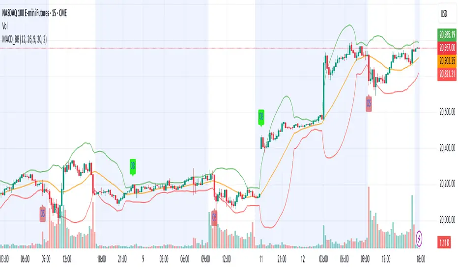
Ichimoku Score Indicator [tanayroy]The Ichimoku Cloud is a comprehensive indicator that provides a clear view of market states through five key components. By analyzing the interaction between these components and the asset's price, traders can gain insights into trend direction, momentum, and potential reversals.
Introducing the Ichimoku Score System
I have developed a scoring system that quantifies these interactions, offering an objective method to evaluate market conditions. The score is calculated based on the relative positioning of Ichimoku components, with adjustable weightings via user input.
Scoring Criteria
Each component contributes to the overall score as follows:
Price vs. Cloud (Kumo) & Other Components
Price vs. Kumo → 2 Points
Price vs. Kumo Shadow → 0.5 Points
Tenkan vs. Kijun
Tenkan vs. Kijun → 2 Points
Tenkan vs. Kumo → 0.5 Points
Kijun vs. Kumo → 0.5 Points
Tenkan Slope → 0.5 Points
Kijun Slope → 0.5 Points
Chikou Span Interactions
Price vs. Chikou → 2 Points
Chikou vs. Kumo → 0.5 Points
Chikou Consolidation → 0.5 Points
Senkou Span Analysis
Senkou A vs. Senkou B → 2 Points
Senkou Slope → 0.5 Points
Price vs. Key Levels
Price vs. Tenkan → 2 Points
Price vs. Kijun → 2 Points
Interpreting the Score
The aggregate score functions as an oscillator, fluctuating between a range of ±16.0.
A higher score indicates strong bullish momentum.
A lower score suggests bearish market conditions.
To enhance readability and smooth fluctuations, a 9-period SMA is applied to the score.
Application in Algorithmic Trading
This scoring system helps integrate Ichimoku Cloud principles into algorithmic trading strategies by providing a structured and quantifiable method for assessing market conditions.
Would love to hear your feedback! 🚀 Let me know how this system works for you.
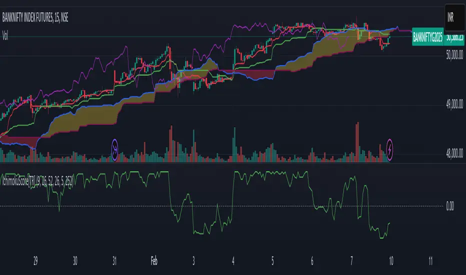
Weekly RSI Buy/Sell SignalsWeekly RSI Buy/Sell Signal Indicator
This indicator is designed to help traders identify high-probability buy and sell opportunities on the weekly chart by using the Relative Strength Index (RSI). By utilizing weekly RSI values, this indicator ensures signals align with broader market trends, providing a clearer view of potential price reversals and continuation.
How It Works:
Weekly RSI Calculation: This script calculates the RSI using a 14-period setting, focusing on the weekly timeframe regardless of the user’s current chart view. The weekly RSI is derived using request.security, allowing for consistent signals even on intraday charts.
Signal Conditions:
Buy Signal: A buy signal appears when the RSI crosses above the oversold threshold of 30, suggesting that price may be gaining momentum after a potential bottom.
Sell Signal: A sell signal triggers when the RSI crosses below the overbought threshold of 70, indicating a possible momentum shift downwards.
Visual Cues:
Buy/Sell Markers: Clear green "BUY" and red "SELL" markers are displayed on the chart when buy or sell conditions are met, making it easy to identify entry and exit points.
RSI Line and Thresholds: The weekly RSI value is plotted in real time with color-coded horizontal lines at 30 (oversold) and 70 (overbought), providing a visual reference for key levels.
This indicator is ideal for traders looking for reliable, trend-based signals on higher timeframes and can be a helpful tool for filtering out shorter-term market noise.
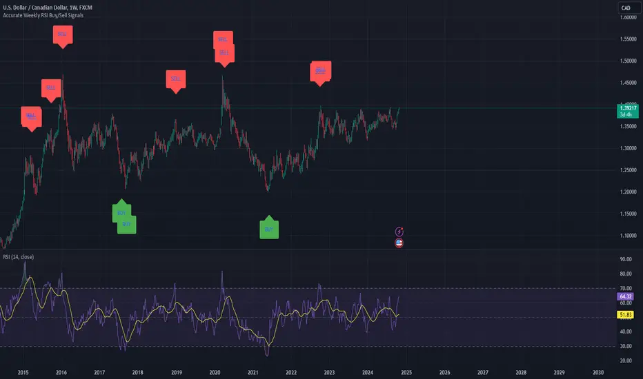
Rolling Straddle PremiumScript is Basically intended to provide insight's on the Rolling Straddle premium for the selected index based on the input settings.
Important thing to consider for the script to work seamlessly:
Specify the LTP in the input field (need not be very accurate)
Specify the Expiry Date for the Option Strike.
Ensure Profile matches to the chart script (Index Script)
Note: Zones marked in Blue, is the max level that indicator can track the option prices. beyond which it may fail to track, during such time consider reloading the indicator with Latest LTP .
Labels on the chart indicate that If i had shorted the Straddle, what would be my current position of that Straddle. however the rational behind shorting is only the pivot high points (not sure if this is right or wrong! )
Note On Labels: Labels are delayed basis the pivot point candles specified in the indicator settings.
EN: Entry Price (Straddle Premium) of the Strike Specified.
Cur: Current Price ( Current Straddle Premium ) of the Strike Specified.
SH: Max Straddle Premium ( Increase in Premium ) since position is active.
SL: Min Straddle Premium ( Premium Erosion ) since position is active.
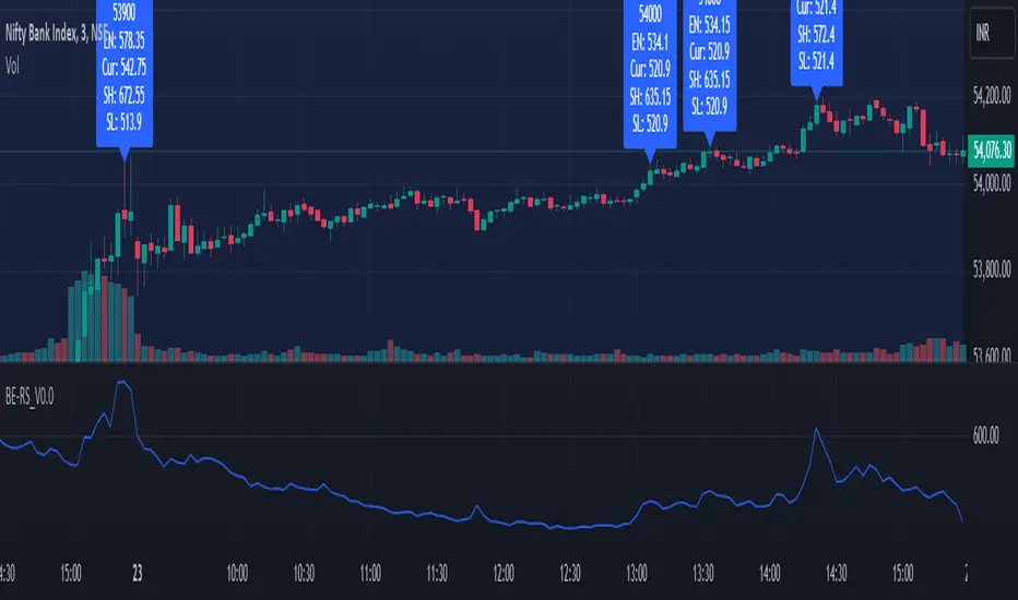
Approximate Spectral Entropy-Based Market Momentum (SEMM)Overview
The Approximate Spectral Entropy-Based Market Momentum (SEMM) indicator combines the concepts of spectral entropy and traditional momentum to provide traders with insights into both the strength and the complexity of market movements. By measuring the randomness or predictability of price changes, SEMM helps traders understand whether the market is in a trending or consolidating state and how strong that trend or consolidation might be.
Key Features
Entropy Measurement: Calculates the approximate spectral entropy of price movements to quantify market randomness.
Momentum Analysis: Integrates entropy with rate-of-change (ROC) to highlight periods of strong or weak momentum.
Dynamic Market Insight: Provides a dual perspective on market behavior—both the trend strength and the underlying complexity.
Customizable Parameters: Adjustable window length for entropy calculation, allowing for fine-tuning to suit different market conditions.
Concepts Underlying the Calculations
The indicator utilizes Shannon entropy, a concept from information theory, to approximate the spectral entropy of price returns. Spectral entropy traditionally involves a Fourier Transform to analyze the frequency components of a signal, but due to Pine Script limitations, this indicator uses a simplified approach. It calculates log returns over a rolling window, normalizes them, and then computes the Shannon entropy. This entropy value represents the level of disorder or complexity in the market, which is then multiplied by traditional momentum measures like the rate of change (ROC).
How It Works
Price Returns Calculation: The indicator first computes the log returns of price data over a specified window length.
Entropy Calculation: These log returns are normalized and used to calculate the Shannon entropy, representing market complexity.
Momentum Integration: The calculated entropy is then multiplied by the rate of change (ROC) of prices to generate the SEMM value.
Signal Generation: High SEMM values indicate strong momentum with higher randomness, while low SEMM values indicate lower momentum with more predictable trends.
How Traders Can Use It
Trend Identification: Use SEMM to identify strong trends or potential trend reversals. Low entropy values can indicate a trending market, whereas high entropy suggests choppy or consolidating conditions.
Market State Analysis: Combine SEMM with other indicators or chart patterns to confirm the market's state—whether it's trending, ranging, or transitioning between states.
Risk Management: Consider high SEMM values as a signal to be cautious, as they suggest increased market unpredictability.
Example Usage Instructions
Add the Indicator: Apply the "Approximate Spectral Entropy-Based Market Momentum (SEMM)" indicator to your chart.
Adjust Parameters: Modify the length parameter to suit your trading timeframe. Shorter lengths are more responsive, while longer lengths smooth out the signal.
Analyze the Output: Observe the blue line for entropy and the red line for SEMM. Look for divergences or confirmations with price action to guide your trades.
Combine with Other Tools: Use SEMM alongside moving averages, support/resistance levels, or other indicators to build a comprehensive trading strategy.
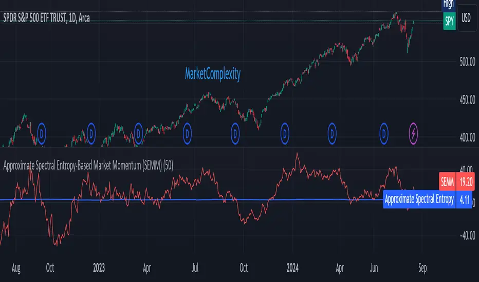
Multi-Spectral RSI Deviations [AlgoAlpha]🌌 Multi-Spectral RSI Deviations by AlgoAlpha - Dive into Market Dynamics! 🌠
Dive deep into the essence of market trends with our 🚀 Multi-Spectral RSI Deviations indicator, a comprehensive tool designed by AlgoAlpha to enhance your trading strategy. By harnessing the power of multiple RSI lengths and innovative smoothing techniques, this indicator offers a unique perspective on market momentum and potential reversals.
🔍 Key Features:
🎨 Customizable up and down colors for immediate trend recognition.
🔢 Three RSI lengths for multi-layered market analysis.
🔄 Various Moving Average (MA) types including SMA, EMA, and more for tailored smoothing.
✅ Bullish and Bearish divergence plotting for spotting potential reversals.
🕵️♂️ Adjustable divergence sensitivity settings to fine-tune signal detection.
🔔 Built-in alerts for trend shifts and reversal conditions, ensuring you never miss a trading opportunity.
🚀 Quick Guide to Using the Multi-Spectral RSI Deviations Indicator
🛠 Add the Indicator: Search for "Multi-Spectral RSI Deviations" in TradingView's Indicators & Strategies. Adjust the RSI lengths and MA settings to suit your trading strategy.
🔍 Market Analysis: Keep an eye on the color changes for trend direction and use divergence plots to anticipate potential market reversals.
🔔 Alerts Setup: Activate the built-in alerts for trend shifts and reversals to stay ahead of the game without having to constantly monitor the charts.
🧠 How It Works:
At the core of the Multi-Spectral RSI Deviations indicator is its ability to analyze the market through various RSI lengths, providing a comprehensive view of momentum. The indicator calculates the Relative Strength Index (RSI) over three different periods, creating a spectrum of momentum insights. These RSI values are then compared to each other to identify the momentum shifts within the market.
To refine these insights, the differences between these RSI values are smoothed using a selected Moving Average type, such as SMA, EMA, etc., based on user preference. This smoothing process helps in highlighting the overall trend direction and potential reversal points with greater clarity.
Furthermore, the indicator employs a color-coding system, where the plotted line changes color based on the momentum's direction—shifting to an up color for positive momentum and a down color for negative momentum. This visual cue enables traders to quickly discern the market trend at a glance.
Divergences between the price action and the indicator's values are another cornerstone of this tool. By plotting potential bullish and bearish divergences, the indicator provides early signals of possible trend reversals, offering traders a strategic advantage.
Embrace the power of our 🌌 Multi-Spectral RSI Deviations and elevate your trading to stellar heights! 🌠✨

Enhanced Candle Sticks [AlgoAlpha]🚀🌟 Introducing the Enhanced Candle Sticks by AlgoAlpha, a Pine Script tool designed to provide traders with an enhanced view of market dynamics through candlestick analysis. This script aims to visualise if price has hit the high or low of the candle first, aiding in back-testing, and to identify smaller trends using market structure.📊🔍
Key Features:
Timeframe Flexibility: Users can select their desired timeframe for analysis, offering a range of options from M15 to H12. This flexibility allows for detailed and specific timeframe analysis.
Micro Trend Identification: The script includes an option to enable 'MicroTrends', giving traders insights into smaller movements and trends within the larger market context.
Customizable Visuals: Traders can customize the colors of bullish and bearish candlesticks, enhancing visual clarity and personalizing the chart to their preferences.
State Tracking: The script tracks the 'state' of the market on lower timeframes to detect if the high or the low was formed first.
Warning System: When the selected timeframe does not match the chart timeframe, the script generates a warning, ensuring accurate analysis and preventing potential misinterpretations.
Usages:
Enhanced Back-testing: Users can now get a more accurate interpretation of the candlesticks by know if the high or the low came first (denoted with ⩚ or ⩛), especially in scenarios where the high and the low of the larger timeframe candle is touching both the take-profit and stop-loss levels.
Squeeze Analysis: Users can identify squeezes in price when the microtrend shows both an uptrend and a downtrend, possibly giving more insight into the market.
Lower Timeframe Market Structure Analysis: Microtrends form when the low of the candle is consecutively increasing and the high is consecutively falling, which means on a lower timeframe, price is forming higher lows or lower highs.
Basic Logic Explanation:
- The script starts by setting up the necessary parameters and importing the required library. Users can customize the timeframe, colors, and whether to enable micro trends and candlestick plotting.
- It then calculates the lower timeframe (1/12th of the current timeframe) for more detailed analysis. The `minutes` function helps in converting the selected timeframe into minutes.
- The script tracks new bars and calculates the highest and lowest values within an hour, using `ta.highestSince` and `ta.lowestSince`.
- It determines the market 'state' by checking if the current high is breaking the previous high and if the current low is breaking the previous low on lower timeframes to determine if the high or the low was formed first.
- The script uses the `plotchar` and `plotcandle` functions to visually represent these trends and states on the chart. This visual representation is key for quick and effective analysis.
Alerts:
Alerts can be set for microtrend formations:
This script is a valuable tool for traders looking to deepen their market analysis with enhanced candlestick visualization and micro trend tracking. 📈🔶💡
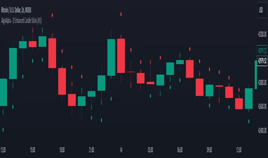
Standardized Median Proximity [AlgoAlpha]Introducing the Standardized Median Proximity by AlgoAlpha 🚀📊 – a dynamic tool designed to enhance your trading strategy by analyzing price fluctuations relative to the median value. This indicator is built to provide clear visual cues on the price deviation from its median, allowing for a nuanced understanding of market trends and potential reversals.
🔍 Key Features:
1. 📈 Median Tracking: At the core of this indicator is the calculation of the median price over a specified lookback period. By evaluating the current price against this median, the indicator provides a sense of whether the price is trending above or below its recent median value.
medianValue = ta.median(priceSource, lookbackLength)
2. 🌡️ Normalization of Price Deviation: The deviation of the price from the median is normalized using standard deviation, ensuring that the indicator's readings are consistent and comparable across different time frames and instruments.
standardDeviation = ta.stdev(priceDeviation, 45)
normalizedValue = priceDeviation / (standardDeviation + standardDeviation)
3. 📌 Boundary Calculations: The indicator sets upper and lower boundaries based on the normalized values, helping to identify overbought and oversold conditions.
upperBoundary = ta.ema(positiveValues, lookbackLength) + ta.stdev(positiveValues, lookbackLength) * stdDevMultiplier
lowerBoundary = ta.ema(negativeValues, lookbackLength) - ta.stdev(negativeValues, lookbackLength) * stdDevMultiplier
4. 🎨 Visual Appeal and Clarity: With carefully chosen colors, the plots provide an intuitive and clear representation of market states. Rising trends are indicated in a shade of green, while falling trends are shown in red.
5. 🚨 Alert Conditions: Stay ahead of market movements with customizable alerts for trend shifts and impulse signals, enabling timely decisions.
alertcondition(ta.crossover(normalizedValue, 0), "Bullish Trend Shift", "Median Proximity Crossover Zero Line")
🔧 How to Use:
- 🎯 Set your preferred lookback lengths and standard deviation multipliers to tailor the indicator to your trading style.
- 💹 Utilize the boundary plots to understand potential overbought or oversold conditions.
- 📈 Analyze the color-coded column plots for quick insights into the market's direction relative to the median.
- ⏰ Set alerts to notify you of significant trend changes or conditions that match your trading criteria.
Basic Logic Explained:
- The indicator first calculates the median of the selected price source over your chosen lookback period. This median serves as a baseline for measuring price deviation.
- It then standardizes this deviation by dividing it by the standard deviation of the price deviation over a 45-period lookback, creating a normalized value.
- Upper and lower boundaries are computed using the exponential moving average (EMA) and standard deviation of these normalized values, adjusted by your selected multiplier.
- Finally, color-coded plots provide a visual representation of these calculations, offering at-a-glance insights into market conditions.
Remember, while this tool offers valuable insights, it's crucial to use it as part of a comprehensive trading strategy, complemented by other analysis and indicators. Happy trading!
🚀
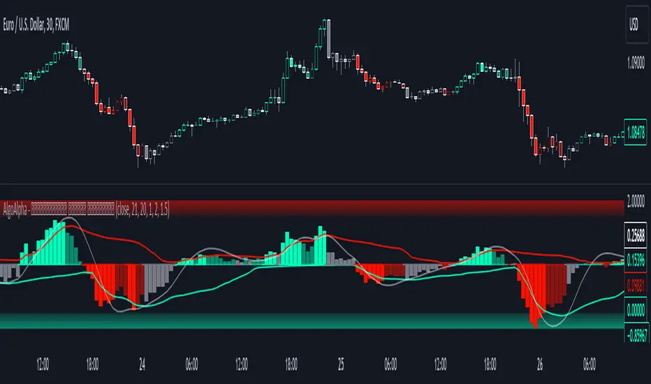
Median Proximity Percentile [AlgoAlpha]📊🚀 Introducing the "Median Proximity Percentile" by AlgoAlpha, a dynamic and sophisticated trading indicator designed to enhance your market analysis! This tool efficiently tracks median price proximity over a specified lookback period and finds it's percentile between 2 dynamic standard deviation bands, offering valuable insights for traders looking to make informed decisions.
🌟 Key Features:
Color-Coded Visuals: Easily interpret market trends with color-coded plots indicating bullish or bearish signals.
Flexibility: Customize the indicator with your preferred price source and lookback lengths to suit your trading strategy.
Advanced Alert System: Stay ahead with customizable alerts for key trend shifts and market conditions.
🔍 Deep Dive into the Code:
Choose your preferred price data source and define lookback lengths for median and EMA calculations. priceSource = input.source(close, "Source") and lookbackLength = input.int(21, minval = 1, title = "Lookback Length")
Calculate median value, price deviation, and normalized value to analyze market position relative to the median. medianValue = ta.median(priceSource, lookbackLength)
Determine upper and lower boundaries based on standard deviation and EMA. upperBoundary = ta.ema(positiveValues, lookbackLength) + ta.stdev(positiveValues, lookbackLength) * stdDevMultiplier
lowerBoundary = ta.ema(negativeValues, lookbackLength) - ta.stdev(negativeValues, lookbackLength) * stdDevMultiplier
Compute the percentile value to track market position within these boundaries. percentileValue = 100 * (normalizedValue - lowerBoundary)/(upperBoundary - lowerBoundary) - 50
Enhance your analysis with Hull Moving Average (HMA) for smoother trend identification. emaValue = ta.hma(percentileValue, emaLookbackLength)
Visualize trends with color-coded plots and characters for easy interpretation. plotColor = percentileValue > 0 ? colorUp : percentileValue < 0 ? colorDown : na
Set up advanced alerts to stay informed about significant market movements. // Alerts
alertcondition(ta.crossover(emaValue, 0), "Bullish Trend Shift", "Median Proximity Percentile Crossover Zero Line")
alertcondition(ta.crossunder(emaValue, 0), "Bearish Trend Shift", "Median Proximity Percentile Crossunder Zero Line")
alertcondition(ta.crossunder(emaValue,emaValue ) and emaValue > 90, "Bearish Reversal", "Median Proximity Percentile Bearish Reversal")
alertcondition(ta.crossunder(emaValue ,emaValue) and emaValue < -90, "Bullish Reversal", "Median Proximity Percentile Bullish Reversal")
🚨 Remember, the "Median Proximity Percentile " is a tool to aid your analysis. It’s essential to combine it with other analysis techniques and market understanding for best results. Happy trading! 📈📉

Momentum Bias Index [AlgoAlpha]Description:
The Momentum Bias Index by AlgoAlpha is designed to provide traders with a powerful tool for assessing market momentum bias. The indicator calculates the positive and negative bias of momentum to gauge which one is greater to determine the trend.
Key Features:
Comprehensive Momentum Analysis: The script aims to detect momentum-trend bias, typically when in an uptrend, the momentum oscillator will oscillate around the zero line but will have stronger positive values than negative values, similarly for a downtrend the momentum will have stronger negative values. This script aims to quantify this phenomenon.
Overlay Mode: Traders can choose to overlay the indicator on the price chart for a clear visual representation of market momentum.
Take-profit Signals: The indicator includes signals to lock in profits, they appear as labels in overlay mode and as crosses when overlay mode is off.
Impulse Boundary: The script includes an impulse boundary, the impulse boundary is a threshold to visualize significant spikes in momentum.
Standard Deviation Multiplier: Users can adjust the standard deviation multiplier to increase the noise tolerance of the impulse boundary.
Bias Length Control: Traders can customize the length for evaluating bias, enabling them to fine-tune the indicator according to their trading preferences. A higher length will give a longer-term bias in trend.
Squeeze & Release [AlgoAlpha]Introduction:
💡The Squeeze & Release by AlgoAlpha is an innovative tool designed to capture price volatility dynamics using a combination of EMA-based calculations and ATR principles. This script aims to provide traders with clear visual cues to spot potential market squeezes and release scenarios. Hence it is important to note that this indicator shows information on volatility, not direction.
Core Logic and Components:
🔶EMA Calculations: The script utilizes the Exponential Moving Average (EMA) in multiple ways to smooth out the data and provide indicator direction. There are specific lengths for the EMAs that users can modify as per their preference.
🔶ATR Dynamics: Average True Range (ATR) is a core component of the script. The differential between the smoothed ATR and its EMA is used to plot the main line. This differential, when represented as a percentage of the high-low range, provides insights into volatility.
🔶Squeeze and Release Detection: The script identifies and highlights squeeze and release scenarios based on the crossover and cross-under events between our main line and its smoothed version. Squeezes are potential setups where the market may be consolidating, and releases indicate a potential breakout or breakdown.
🔶Hyper Squeeze Detection: A unique feature that detects instances when the main line is rising consistently over a user-defined period. Hyper squeeze marks areas of extremely low volatility.
Visual Components:
The main line (ATR-based) changes color depending on its position relative to its EMA.
A middle line plotted at zero level which provides a quick visual cue about the main line's position. If the main line is above the zero level, it indicates that the price is squeezing on a longer time horizon, even if the indicator indicates a shorter-term release.
"𝓢" and "𝓡" characters are plotted to represent 'Squeeze' and 'Release' scenarios respectively.
Standard Deviation Bands are plotted to help users gauge the extremity and significance of the signal from the indicator, if the indicator is closer to either the upper or lower deviation bands, this means that statistically, the current value is considered to be more extreme and as it is further away from the mean where the indicator is oscillating at for the majority of the time. Thus indicating that the price has experienced an unusual amount or squeeze or release depending on the value of the indicator.
Usage Guidelines:
☝️Traders can use the script to:
Identify potential consolidation (squeeze) zones.
Gauge potential breakout or breakdown scenarios (release).
Fine-tune their entries and exits based on volatility.
Adjust the various lengths provided in the input for better customization based on individual trading styles and the asset being traded.

Bollinger Bands Percentile + Stdev Channels (BBPct) [AlgoAlpha]Description:
The "Bollinger Bands Percentile (BBPct) + STD Channels" mean reversion indicator, developed by AlgoApha, is a technical analysis tool designed to analyze price positions using Bollinger Bands and Standard Deviation Channels (STDC). The combination of these two indicators reinforces a stronger reversal signal. BBPct calculates the percentile rank of the price's standard deviation relative to a specified lookback period. Standard deviation channels operate by utilizing a moving average as the central line, with upper and lower lines equidistant from the average based on the market's volatility, helping to identify potential price boundaries and deviations.
How it Works:
The BBPct indicator utilizes Bollinger Bands, which consist of a moving average (basis) and upper and lower bands based on a specified standard deviation multiplier. By default, it uses a 20-period moving average and a standard deviation multiplier of 2. The upper band is calculated by adding the basis to the standard deviation multiplied by the multiplier, while the lower band is calculated by subtracting the same value. The BBPct indicator calculates the position of the current price between the lower and upper Bollinger Bands as a percentile value. It determines this position by comparing the price's distance from the lower band to the overall range between the upper and lower bands. A value of 0 indicates that the price is at the lower band, while a value of 100 indicates that the price is at the upper band. The indicator also includes an optional Bollinger Band standard deviation percentage (%Stdev) histogram, representing the deviation of the current price from the moving average as a percentage of the price itself.
Standard deviation channels, also known as volatility channels, aid in identifying potential buying and selling opportunities while minimizing unfavorable trades. These channels are constructed by two lines that run parallel to a moving average. The separation between these lines is determined by the market's volatility, represented by standard deviation. By designating upper and lower channel lines, the channels demarcate the borders between typical and atypical price movements. Consequently, when the market's price falls below the lower channel line, it suggests undervaluation, whereas prices surpassing the upper channel line indicate overvaluation.
Signals
The chart displays potential reversal points through the use of red and green arrows. A red arrow indicates a potential bearish retracement, signaling a possible downward movement, while a green arrow represents a potential pullback to the positive, suggesting a potential upward movement. These signals are generated only when both the BBPct (Bollinger Bands Percentage) and the STDC (Standard Deviation Channel) indicators align with bullish or bearish conditions. Consequently, traders might consider opening long positions when the green arrow appears and short positions when the red arrow is plotted.
Usage:
This indicator can be utilized by traders and investors to effectively identify pullbacks, reversals, and mean regression, thereby enhancing their trading opportunities. Notably, extreme values of the BBPct, such as below -5 or above 105, indicate oversold or overbought conditions, respectively. Moreover, the presence of extreme STDC zones occurs when prices fall below the lower channel line or cross above the upper channel line. Traders can leverage this information as a mean reversion tool by identifying instances of peak overbought and oversold values. These distinctive characteristics facilitate the identification of potential entry and exit points, thus augmenting trading decisions and enhancing market analysis.
The indicator's parameters, such as the length of the moving average, the data source, and the standard deviation multiplier, can be customized to align with individual trading strategies and preferences.
Originality:
The BBPct + STDC indicator, developed by AlgoAlpha, is an original implementation that combines the calculation of Bollinger Bands, percentile ranking, the %Stdev histogram and the STDC. While it shares some similarities with the Bollinger Bands %B indicator, the BBPct indicator introduces additional elements and customization options tailored to AlgoAlpha's methodology. The script is released under the Mozilla Public License 2.0, granting users the freedom to utilize and modify it while adhering to the license terms.
