Crypto McClellan Oscillator (SLN Fix)This is an adaption of the Mcclellan Oscillator for crypto. Instead of tracking the S&P500 it tracks a selection of cryptos to make sure the indicator follows this sector instead.
Full credit goes to the creator of this indicator: Fadior. It has since been fixed by SLN.
The following description explains the standard McClellan Oscillator. Full credit to Investopedia , my fav source of financial explanations.
The same principles applies to its use in the crypto sector, but please be cautious of the last point, the limitations. Since crypto is more volatile, that could amplify choppy behavior.
This is not financial advice, please be extremely cautious. This indicator is only suitable as a confirmation signal and needs support of other signals to be profitable.
This indicator usually produces the best signals on slightly above daily time frame. I personally like 2 or 3 day, but you have to find the settings suitable for your trading style.
What Is the McClellan Oscillator?
The McClellan Oscillator is a market breadth indicator that is based on the difference between the number of advancing and declining issues on a stock exchange, such as the New York Stock Exchange (NYSE) or NASDAQ.
The indicator is used to show strong shifts in sentiment in the indexes, called breadth thrusts. It also helps in analyzing the strength of an index trend via divergence or confirmation.
The McClellan Oscillator formula can be applied to any stock exchange or group of stocks.
A reading above zero helps confirm a rise in the index, while readings below zero confirm a decline in the index.
When the index is rising but the oscillator is falling, that warns that the index could start declining too. When the index is falling and the oscillator is rising, that indicates the index could start rising soon. This is called divergence.
A significant change, such as moving 100 points or more, from a negative reading to a positive reading is called a breadth thrust. It may indicate a strong reversal from downtrend to uptrend is underway on the stock exchange.
How to Calculate the McClellan Oscillator
To get the calculation started, track Advances - Declines on a stock exchange for 19 and 39 days. Calculate a simple average for these, not exponential moving average (EMA).
Use these simple values as the Prior Day EMA values in the 19- and 39-day EMA formulas.
Calculate the 19- and 39-day EMAs.
Calculate the McClellan Oscillator value.
Now that the value has been calculated, on the next calculation use this value for the Prior Day EMA. Start calculating EMAs for the formula instead of simple averages.
If using the adjusted formula, the steps are the same, except use ANA instead of using Advances - Declines.
What Does the McClellan Oscillator Tell You?
The McClellan Oscillator is an indicator based on market breadth which technical analysts can use in conjunction with other technical tools to determine the overall state of the stock market and assess the strength of its current trend.
Since the indicator is based on all the stocks in an exchange, it is compared to the price movements of indexes that reflect that exchange, or compared to major indexes such as the S&P 500.
Positive and negative values indicate whether more stocks, on average, are advancing or declining. The indicator is positive when the 19-day EMA is above the 39-day EMA, and negative when the 19-day EMA is below the 39-day EMA.
A positive and rising indicator suggests that stocks on the exchange are being accumulated. A negative and falling indicator signals that stocks are being sold. Typically such action confirms the current trend in the index.
Crossovers from positive to negative, or vice versa, may signal the trend has changed in the index or exchange being tracked. When the indicator makes a large move, typically of 100 points or more, from negative to positive territory, that is called a breadth thrust.
It means a large number of stocks moved up after a bearish move. Since the stock market tends to rise over time, this a positive signal and may indicate that a bottom in the index is in and prices are heading higher overall.
When index prices and the indicator are moving in different directions, then the current index trend may lack strength. Bullish divergence occurs when the oscillator is rising while the index is falling. This indicates the index could head higher soon since more stocks are starting to advance.
Bearish divergence is when the index is rising and the indicator is falling. This means fewer stocks are keeping the advance going and prices may start to head lower.
Limitations of Using the McClellan Oscillator
The indicator tends to produce lots of signals. Breadth thrusts, divergence, and crossovers all occur with some frequency, but not all these signals will result in the price/index moving in the expected direction.
The indicator is prone to producing false signals and therefore should be used in conjunction with price action analysis and other technical indicators.
The indicator can also be quite choppy, moving between positive and negative territory rapidly. Such action indicates a choppy market, but this isn't evident until the indicator has made this whipsaw move a few times.
Good luck and a big thanks to Fadior!
在脚本中搜索"19亿美元是多少人民币"

Pre-COVID High and COVID LowOverview
The "Pre-COVID High and COVID Low" indicator is designed to identify and mark significant price levels on your chart, specifically targeting the pre-COVID-19 high and the low during the initial COVID-19 market impact. This script is particularly useful for traders who are interested in analyzing how stocks or other financial instruments reacted during the onset of the COVID-19 pandemic, providing a historical perspective that may help in making informed trading decisions.
How It Works
Date Ranges : The script uses predefined date ranges to calculate the highest and lowest price levels before and during the early stages of the COVID-19 pandemic. These ranges are:
Pre-COVID High: Between January 1, 2020, and March 31, 2020.
COVID Low: Between March 1, 2020, and March 31, 2020.
Calculation Method :
The highest price during the pre-COVID period is tracked and recorded as the "Pre-COVID High".
The lowest price during the specified COVID period is tracked and recorded as the "COVID Low".
Visibility Conditions : The script includes logic to ensure that these historical levels are only displayed if they fall within a range close to the current visible price range on the chart. This prevents the indicator from compressing the price scale unduly.
How to Use It
Adding to Your Char t: To use this indicator, add it to any chart on TradingView. It works best with daily time frames to clearly visualize the impact over these specific months.
Interpretation :
The "Pre-COVID High" is marked with a red line and is labeled the first day it becomes applicable.
The "COVID Low" is marked with a green line and is similarly labeled on its applicable day.
Trading Strategy Consideration : Traders can use these historical levels as potential support or resistance zones for their trading strategies. These levels can indicate significant price points where the market previously showed strong reactions.

Baha'i Reversal Points [CC]The Baha'i Reversal Points is a custom creation that combines some of my favorite passions, creating stock indicator scripts and my faith. The Baha'i Faith believes in the oneness of God and all religions, and sees the number 9 as significant because that is the number of major world religions as well as the Baha'i symbol is a nine-pointed star. The number 19 is also seen as significant because in the Baha'i calendar, there are 19 months, and each month is made up of 19 days. Anyway, with all that being explained, I created these reversal points to find the points where the last 19 highs or lows are higher or lower, respectively than the previous high or low nine days ago. As with many indicators, this does have some hits and misses but does a pretty good job of finding reversal points based on these criteria.
There are a few different ways to analyze this data to determine when to buy or sell. I have set the default behavior for when we encounter the first time that the amount of highs or lows is greater than or equal to the length amount using a crossover or crossunder alert. You could also ignore the crossover or crossunder alerts and buy when the count is greater than or equal to the length, which can happen for extended periods depending on the underlying trend. Overall, buy when the buy label appears and sell when the sell label appears.
Let me know if there are any other custom indicators or scripts you would like to see me publish!

TARVIS Labs - Bitcoin Macro Bottom/Top SignalsSCRIPT DESCRIPTION
This is a script specifically written to help provide indicators from a macro view. This script is best run on the 1 day interval on Bitstamp's $BTCUSD chart. It helps indicate when to accumulate bitcoin, and when its in a bull run when there are local tops, strong top warnings, and a signal to exit a bull run. This is described further below.
If you don't have interest in trading on the way to the top I suggest turning off the following indicators in the settings of the indicator:
- Opportunity To Buy Back In Indicator
- Local Top Near Bull Run Top Indicator
ACCUMULATION ZONE INDICATOR - LIGHT GREEN
Description
When we look at the history of Bitcoin every bottom has crossed below the 100 week EMA. Once it does its accompanied by hash ribbon cross with miner capitulation. After that is the prime time to accumulate as theres a clearer signal the bottom is in. Specifically, a signal to look for is the 14 day MACD/signal cross and the 14 day MACD continuing to stay above the signal until the price returns above the 100 week EMA. This is prime accumulation territory.
Strategy for Usage
A good strategy to use when accumulating the bottom is dollar-cost averaging over a 30 day period. The accumulation zone can last longer than 30 days but 30 days is a good range of time to DCA.
STRONG BUY IN ACCUMULATION ZONE INDICATOR - DARK GREEN
Description
We can add to the bottoming signal by looking for post-downtrend reversals inside the bottoming signal. We do this by using a 9/19 daily cross.
Strategy for Usage
These post-downtrend reversals can potentially provide better targeted days for accumulation than the broader bottoming signal and can be used to add more on that day than on an average day for the dollar cost average strategy. Say for example, use 1/3 of funds on these days rather than 1/30th.
OPPORTUNITY TO BUY BACK IN INDICATOR - BLUE
Description
When the 1d 18 EMA > 1d 63 EMA and the 12/52 1d crosses. These together provide good buy opportunities to buy bitcoin.
Strategy for Usage
If you happen to find yourself out of the market from your own TA or a trade, this signal can provide a buy opportunity to reenter the market if you're out of it.
BULL RUN LOCAL TOP INDICATOR - ORANGE
Description
We will similarly use the 100 week EMA to determine trend reversal into a bull run. When we see the 100 week EMA uptrending, we can begin to look for local tops using the 9/19 daily MACD/signal bearish cross along with the 12 EMA having a negative slope, which could be the beginning signal for a local top.
Strategy for Usage
This is a rather light indicator, but can be used in tandem with your own technical analysis to determine if you want to reenter after you exit from its signal.
LOCAL TOP NEAR BULL RUN TOP INDICATOR - RED
Description
When the 100 week EMA is in an uptrend we can look for significant loss of momentum in order to determine if a local top is in near a bull run top. Similar to the Bull Run Local Top Indicator, this strategy uses a MACD/signal cross but instead uses the 30/65 day EMAs.
Strategy for Usage
Ideally the right strategy to use here is to exit the market when this indicator starts. When the indicator ends if the "End of Bull Run Indicator" is not showing on the chart you can buy back into the market.
TOP IS LIKELY IN INDICATOR
Description
When the 100 week EMA is in a very strong uptrend and the 9/19 weekly MACD/signal bearish cross occurs, and the 63 EMA begins to downtrend.
Strategy for Usage
This signal typically accompanies the "Local Top Near Bull Run Top Indicator" therefore if you're following the strategy you would likely already be out of the market, but if you're not and this signal fires its a strong signal the top is in and we're likely going to start seeing a strong retrace. This is typically right before we see the "End of Bull Run Indicator". There is only one occurrence where it wasn't followed by a large drop & the "End of Bull Run Indicator" and that was in the 2017 bull run where there were many strong retracements post local top. The likelihood we see that again is low, but if it were to happen you can buy back into the market when the "Top is Likely In Indicator" and the "Local Top Near Bull Run Top Indicator" are not firing.
TOP IS LIKELY IN INDICATOR
Description
When the 100 week EMA is in a strong uptrend and the 9/19 weekly MACD/signal bearish cross occurs, and the 63 EMA begins to downtrend.
Strategy for Usage
This signal typically accompanies the "Local Top Near Bull Run Top Indicator" therefore if you're following the strategy you would likely already be out of the market, but if you're not and this signal fires its a strong signal the top is in and we're likely going to start seeing a strong retrace. This is typically right before we see the "End of Bull Run Indicator". There is only one occurrence where it wasn't followed by a large drop & the "End of Bull Run Indicator" and that was in the 2017 bull run where there were many strong retracements post local top. The likelihood we see that again is low, but if it were to happen you can buy back into the market when the "Top is Likely In Indicator" and the "Local Top Near Bull Run Top Indicator" are not firing.
END OF BULL RUN INDICATOR
Description
When the 100 week EMA is in an uptrend and the 1d 18 EMA crosses the 1d 63 EMA.
Strategy for Usage
When the 100 week EMA is a strong uptrend and the 18/63 cross occurs the top is very likely in. It has occurred in every bull run top leading to the bear market.

TLP Swing Chart V2// This source code is subject to the terms of the Mozilla Public License 2.0 at mozilla.org
// Sửa đổi trên code gốc của © meomeo105
// © meomeo105
//@version=5
indicator('TLP Swing Chart V2', shorttitle='TLP Swing V2', overlay=true, max_lines_count=500)
//-----Input-------
customTF = input.timeframe(defval="",title = "Show Other TimeFrame")
showTLP = input.bool(false, 'Show TLP', inline = "TLP1")
colorTLP = input.color(color.aqua, '', inline = "TLP1")
showSTLP = input.bool(true, 'Show TLP Swing', inline = "Swing1")
colorSTLP = input.color(color.aqua, '', inline = "Swing1")
showLabel = input.bool(true, 'Show Label TimeFrame')
lineSTLP = input.string(title="",options= ,defval="(─)", inline = "Swing1")
lineStyleSTLP = lineSTLP == "(┈)" ? line.style_dotted : lineSTLP == "(╌)" ? line.style_dashed : line.style_solid
//IOSB
IOSB = "TLPInOutSideBarSetting"
ISB = input(true,group =IOSB, title="showISB")
colorISB = input.color(color.rgb(250, 171, 0), inline = "ISB")
OSB = input(true,group =IOSB, title="showOSB")
colorOSB = input.color(color.rgb(56, 219, 255), inline = "OSB")
ZoneColor = input(defval = color.new(color.orange, 90),group =IOSB, title = "Background Color")
BorderColor = input(defval = color.new(color.orange, 100),group =IOSB, title = "Border Color")
/////////////////
var aCZ = array.new_float(0)
float highest = high
float lowest = low
if (array.size(aCZ) > 0)
highest := array.get(aCZ, 0)
lowest := array.get(aCZ, 1)
insideBarCondtion = low >= lowest and low <= highest and high >= lowest and high <= highest
if ( insideBarCondtion == true )
array.push(aCZ, high )
array.push(aCZ, low )
if( array.size(aCZ) >= 2 and insideBarCondtion == false )
float maxCZ = array.max(aCZ)
float minCZ = array.min(aCZ)
box.new(bar_index - (array.size(aCZ) / 2) - 1, maxCZ, bar_index - 1, minCZ, bgcolor = ZoneColor, border_color = BorderColor)
array.clear(aCZ)
//////////////////////////Global//////////////////////////
var arrayLineTemp = array.new_line()
// Funtion
f_resInMinutes() =>
_resInMinutes = timeframe.multiplier * (
timeframe.isseconds ? 1. / 60. :
timeframe.isminutes ? 1. :
timeframe.isdaily ? 1440. :
timeframe.isweekly ? 10080. :
timeframe.ismonthly ? 43800. : na)
// Converts a resolution expressed in minutes into a string usable by "security()"
f_resFromMinutes(_minutes) =>
_minutes < 1 ? str.tostring(math.round(_minutes*60)) + "S" :
_minutes < 60 ? str.tostring(math.round(_minutes)) + "m" :
_minutes < 1440 ? str.tostring(math.round(_minutes/60)) + "H" :
_minutes < 10080 ? str.tostring(math.round(math.min(_minutes / 1440, 7))) + "D" :
_minutes < 43800 ? str.tostring(math.round(math.min(_minutes / 10080, 4))) + "W" :
str.tostring(math.round(math.min(_minutes / 43800, 12))) + "M"
f_tfRes(_res,_exp) =>
request.security(syminfo.tickerid,_res,_exp,lookahead=barmerge.lookahead_on)
var label labelError = label.new(bar_index, high, text = "", color = #00000000, textcolor = color.white,textalign = text.align_left)
sendError(_mmessage) =>
label.set_xy(labelError, bar_index + 3, close )
label.set_text(labelError, _mmessage)
var arrayLineChoCh = array.new_line()
var label labelTF = label.new(time, close, text = "",color = color.new(showSTLP ? colorSTLP : colorTLP,95), textcolor = showSTLP ? colorSTLP : colorTLP,xloc = xloc.bar_time, textalign = text.align_left)
//////////////////////////TLP//////////////////////////
var arrayXTLP = array.new_int(5,time)
var arrayYTLP = array.new_float(5,close)
var arrayLineTLP = array.new_line()
int drawLineTLP = 0
_high = high
_low = low
_close = close
_open = open
if(customTF != timeframe.period)
_high := f_tfRes(customTF,high)
_low := f_tfRes(customTF,low)
_close := f_tfRes(customTF,close)
_open := f_tfRes(customTF,open)
highPrev = _high
lowPrev = _low
// drawLineTLP => 2:Tiếp tục 1:Đảo chiều; // Outsidebar 2:Tiếp tục 3:Tiếp tục và Đảo chiều 4 : Đảo chiều 2 lần
drawLineTLP := 0
if(_high > highPrev and _low > lowPrev )
if(array.get(arrayYTLP,0) > array.get(arrayYTLP,1))
if(_high <= high)
array.set(arrayXTLP, 0, time)
array.set(arrayYTLP, 0, _high )
drawLineTLP := 2
else
array.unshift(arrayXTLP,time)
array.unshift(arrayYTLP,_high )
drawLineTLP := 1
else if(_high < highPrev and _low < lowPrev )
if(array.get(arrayYTLP,0) > array.get(arrayYTLP,1))
array.unshift(arrayXTLP,time)
array.unshift(arrayYTLP,_low )
drawLineTLP := 1
else
if(_low >= low)
array.set(arrayXTLP, 0, time)
array.set(arrayYTLP, 0, _low )
drawLineTLP := 2
else if(_high >= highPrev and _low < lowPrev or _high > highPrev and _low <= lowPrev )
if(array.get(arrayYTLP,0) > array.get(arrayYTLP,1))
if(_high >= array.get(arrayYTLP,0) and array.get(arrayYTLP,1) < _low )
if(_high <= high)
array.set(arrayXTLP, 0, time)
array.set(arrayYTLP, 0, _high )
drawLineTLP := 2
else if(_high >= array.get(arrayYTLP,0) and array.get(arrayYTLP,1) > _low )
if(_close < _open)
if(_high <= high)
array.set(arrayXTLP, 0, time)
array.set(arrayYTLP, 0, _high )
array.unshift(arrayXTLP,time)
array.unshift(arrayYTLP,_low )
drawLineTLP := 3
else
array.unshift(arrayXTLP,time)
array.unshift(arrayYTLP,_low )
array.unshift(arrayXTLP,time)
array.unshift(arrayYTLP,_high )
drawLineTLP := 4
else if(array.get(arrayYTLP,0) < array.get(arrayYTLP,1))
if(_low <= array.get(arrayYTLP,0) and _high < array.get(arrayYTLP,1))
if(_low >= low)
array.set(arrayXTLP, 0, time)
array.set(arrayYTLP, 0, _low )
drawLineTLP := 2
else if(_low <= array.get(arrayYTLP,0) and _high > array.get(arrayYTLP,1))
if(_close > _open)
if(_low >= low)
array.set(arrayXTLP, 0, time)
array.set(arrayYTLP, 0, _low )
array.unshift(arrayXTLP,time)
array.unshift(arrayYTLP,_high )
drawLineTLP := 3
else
array.unshift(arrayXTLP,time)
array.unshift(arrayYTLP,_high )
array.unshift(arrayXTLP,time)
array.unshift(arrayYTLP,_low )
drawLineTLP := 4
else if((_high <= highPrev and _low >= lowPrev ))
highPrev := highPrev
lowPrev := lowPrev
if(f_resInMinutes() < f_tfRes(customTF,f_resInMinutes()) and drawLineTLP == 0)
if(array.get(arrayYTLP,0) > array.get(arrayYTLP,1))
if(array.get(arrayYTLP,0) <= high)
array.set(arrayXTLP, 0, time)
drawLineTLP := 2
else
if(array.get(arrayYTLP,0) >= low)
array.set(arrayXTLP, 0, time)
drawLineTLP := 2
if((showSTLP or showTLP) and f_resInMinutes() <= f_tfRes(customTF,f_resInMinutes()))
if(drawLineTLP == 2)
if(array.size(arrayLineTLP) >0)
line.set_xy2(array.get(arrayLineTLP,0),array.get(arrayXTLP,0),array.get(arrayYTLP,0))
else
array.unshift(arrayLineTLP,line.new(array.get(arrayXTLP,1),array.get(arrayYTLP,1),array.get(arrayXTLP,0),array.get(arrayYTLP,0), color = colorTLP,xloc = xloc.bar_time, style = lineStyleSTLP))
else if(drawLineTLP == 1)
array.unshift(arrayLineTLP,line.new(array.get(arrayXTLP,1),array.get(arrayYTLP,1),array.get(arrayXTLP,0),array.get(arrayYTLP,0), color = colorTLP,xloc = xloc.bar_time, style = lineStyleSTLP))
else if(drawLineTLP == 3)
if(array.size(arrayLineTLP) >0)
line.set_xy2(array.get(arrayLineTLP,0),array.get(arrayXTLP,1),array.get(arrayYTLP,1))
else
array.unshift(arrayLineTLP,line.new(array.get(arrayXTLP,2),array.get(arrayYTLP,2),array.get(arrayXTLP,1),array.get(arrayYTLP,1), color = colorTLP,xloc = xloc.bar_time, style = lineStyleSTLP))
array.unshift(arrayLineTLP,line.new(array.get(arrayXTLP,1),array.get(arrayYTLP,1),array.get(arrayXTLP,0),array.get(arrayYTLP,0), color = colorTLP,xloc = xloc.bar_time, style = lineStyleSTLP))
else if(drawLineTLP == 4)
array.unshift(arrayLineTLP,line.new(array.get(arrayXTLP,2),array.get(arrayYTLP,2),array.get(arrayXTLP,1),array.get(arrayYTLP,1), color = colorTLP,xloc = xloc.bar_time, style = lineStyleSTLP))
array.unshift(arrayLineTLP,line.new(array.get(arrayXTLP,1),array.get(arrayYTLP,1),array.get(arrayXTLP,0),array.get(arrayYTLP,0), color = colorTLP,xloc = xloc.bar_time, style = lineStyleSTLP))
//////////////////////////Swing TLP//////////////////////////
var arrayXSTLP = array.new_int(5,time)
var arrayYSTLP = array.new_float(5,close)
var arrayLineSTLP = array.new_line()
int drawLineSTLP = 0
int drawLineSTLP1 = 0
if(showSTLP)
if(math.max(array.get(arrayYSTLP,0),array.get(arrayYSTLP,1)) < math.min(array.get(arrayYTLP,0),array.get(arrayYTLP,1)) or math.min(array.get(arrayYSTLP,0),array.get(arrayYSTLP,1)) > math.max(array.get(arrayYTLP,0),array.get(arrayYTLP,1)))
//Khởi tạo bắt đầu
drawLineSTLP1 := 5
array.set(arrayXSTLP, 0, array.get(arrayXTLP,1))
array.set(arrayYSTLP, 0, array.get(arrayYTLP,1))
array.unshift(arrayXSTLP,array.get(arrayXTLP,0))
array.unshift(arrayYSTLP,array.get(arrayYTLP,0))
// drawLineSTLP kiểm tra điểm 1 => 13:Tiếp tục có sóng hồi // 12|19(reDraw):Tiếp tục không có sóng hồi // 14:Đảo chiều
if(array.get(arrayXTLP,0) == array.get(arrayXTLP,1))
if(array.get(arrayXSTLP,0) >= array.get(arrayXTLP,2) and array.get(arrayYSTLP,0) != array.get(arrayYTLP,1) and ((array.get(arrayYTLP,1) > array.get(arrayYTLP,2) and array.get(arrayYSTLP,0) > array.get(arrayYSTLP,1)) or (array.get(arrayYTLP,1) < array.get(arrayYTLP,2) and array.get(arrayYSTLP,0) < array.get(arrayYSTLP,1))))
drawLineSTLP1 := 12
array.set(arrayXSTLP, 0, array.get(arrayXTLP,1))
array.set(arrayYSTLP, 0, array.get(arrayYTLP,1))
else if(array.get(arrayXSTLP,0) <= array.get(arrayXTLP,2))
if((array.get(arrayYSTLP,0) > array.get(arrayYSTLP,1) and array.get(arrayYTLP,1) < array.get(arrayYSTLP,1)) or (array.get(arrayYSTLP,0) < array.get(arrayYSTLP,1) and array.get(arrayYTLP,1) > array.get(arrayYSTLP,1)))
drawLineSTLP1 := 14
array.unshift(arrayXSTLP,array.get(arrayXTLP,1))
array.unshift(arrayYSTLP,array.get(arrayYTLP,1))
else if((array.get(arrayYSTLP,0) > array.get(arrayYSTLP,1) and array.get(arrayYTLP,1) > array.get(arrayYSTLP,0)) or (array.get(arrayYSTLP,0) < array.get(arrayYSTLP,1) and array.get(arrayYTLP,1) < array.get(arrayYSTLP,0)))
drawLineSTLP1 := 13
_max = math.min(array.get(arrayYSTLP,0),array.get(arrayYSTLP,1))
_min = math.max(array.get(arrayYSTLP,0),array.get(arrayYSTLP,1))
_max_idx = 0
_min_idx = 0
for i = 2 to array.size(arrayXTLP)
if(array.get(arrayXSTLP,0) >= array.get(arrayXTLP,i))
break
if(_min > array.get(arrayYTLP,i))
_min := array.get(arrayYTLP,i)
_min_idx := array.get(arrayXTLP,i)
if(_max < array.get(arrayYTLP,i))
_max := array.get(arrayYTLP,i)
_max_idx := array.get(arrayXTLP,i)
if(array.get(arrayYSTLP,0) > array.get(arrayYSTLP,1))
array.unshift(arrayXSTLP,_min_idx)
array.unshift(arrayYSTLP,_min)
else if(array.get(arrayYSTLP,0) < array.get(arrayYSTLP,1))
array.unshift(arrayXSTLP,_max_idx)
array.unshift(arrayYSTLP,_max)
array.unshift(arrayXSTLP,array.get(arrayXTLP,1))
array.unshift(arrayYSTLP,array.get(arrayYTLP,1))
if(f_resInMinutes() < f_tfRes(customTF,f_resInMinutes()))
if(array.get(arrayYSTLP,0) == array.get(arrayYTLP,1) and array.get(arrayXSTLP,0) != array.get(arrayXTLP,1))
array.set(arrayXSTLP, 0, array.get(arrayXTLP,1))
drawLineSTLP1 := 19
if(f_resInMinutes() <= f_tfRes(customTF,f_resInMinutes()))
if(drawLineSTLP1 == 12 or drawLineSTLP1 == 19)
if(array.size(arrayLineSTLP) >0)
line.set_xy2(array.get(arrayLineSTLP,0),array.get(arrayXSTLP,0),array.get(arrayYSTLP,0))
else
array.unshift(arrayLineSTLP,line.new(array.get(arrayXSTLP,1),array.get(arrayYSTLP,1),array.get(arrayXSTLP,0),array.get(arrayYSTLP,0), color = colorSTLP,xloc = xloc.bar_time))
else if(drawLineSTLP1 == 14)
array.unshift(arrayLineSTLP,line.new(array.get(arrayXSTLP,1),array.get(arrayYSTLP,1),array.get(arrayXSTLP,0),array.get(arrayYSTLP,0), color = colorSTLP,xloc = xloc.bar_time))
else if(drawLineSTLP1 == 13)
array.unshift(arrayLineSTLP,line.new(array.get(arrayXSTLP,2),array.get(arrayYSTLP,2),array.get(arrayXSTLP,1),array.get(arrayYSTLP,1), color = colorSTLP,xloc = xloc.bar_time))
array.unshift(arrayLineSTLP,line.new(array.get(arrayXSTLP,1),array.get(arrayYSTLP,1),array.get(arrayXSTLP,0),array.get(arrayYSTLP,0), color = colorSTLP,xloc = xloc.bar_time))
else if(drawLineSTLP1 == 15)
if(array.size(arrayLineSTLP) >0)
line.set_xy2(array.get(arrayLineSTLP,0),array.get(arrayXSTLP,1),array.get(arrayYSTLP,1))
else
array.unshift(arrayLineSTLP,line.new(array.get(arrayXSTLP,2),array.get(arrayYSTLP,2),array.get(arrayXSTLP,1),array.get(arrayYSTLP,1), color = colorSTLP,xloc = xloc.bar_time))
array.unshift(arrayLineSTLP,line.new(array.get(arrayXSTLP,1),array.get(arrayYSTLP,1),array.get(arrayXSTLP,0),array.get(arrayYSTLP,0), color = colorSTLP,xloc = xloc.bar_time))
// drawLineSTLP kiểm tra điểm 0 => 3:Tiếp tục có sóng hồi // 2|9(reDraw):Tiếp tục không có sóng hồi // 4:Đảo chiều
if(array.get(arrayXSTLP,0) >= array.get(arrayXTLP,1) and array.get(arrayYSTLP,0) != array.get(arrayYTLP,0) and ((array.get(arrayYTLP,0) > array.get(arrayYTLP,1) and array.get(arrayYSTLP,0) > array.get(arrayYSTLP,1)) or (array.get(arrayYTLP,0) < array.get(arrayYTLP,1) and array.get(arrayYSTLP,0) < array.get(arrayYSTLP,1))))
drawLineSTLP := 2
array.set(arrayXSTLP, 0, array.get(arrayXTLP,0))
array.set(arrayYSTLP, 0, array.get(arrayYTLP,0))
else if(array.get(arrayXSTLP,0) <= array.get(arrayXTLP,1))
if((array.get(arrayYSTLP,0) > array.get(arrayYSTLP,1) and array.get(arrayYTLP,0) < array.get(arrayYSTLP,1)) or (array.get(arrayYSTLP,0) < array.get(arrayYSTLP,1) and array.get(arrayYTLP,0) > array.get(arrayYSTLP,1)))
drawLineSTLP := 4
array.unshift(arrayXSTLP,array.get(arrayXTLP,0))
array.unshift(arrayYSTLP,array.get(arrayYTLP,0))
else if((array.get(arrayYSTLP,0) > array.get(arrayYSTLP,1) and array.get(arrayYTLP,0) > array.get(arrayYSTLP,0)) or (array.get(arrayYSTLP,0) < array.get(arrayYSTLP,1) and array.get(arrayYTLP,0) < array.get(arrayYSTLP,0)))
drawLineSTLP := 3
_max = math.min(array.get(arrayYSTLP,0),array.get(arrayYSTLP,1))
_min = math.max(array.get(arrayYSTLP,0),array.get(arrayYSTLP,1))
_max_idx = 0
_min_idx = 0
for i = 1 to array.size(arrayXTLP)
if(array.get(arrayXSTLP,0) >= array.get(arrayXTLP,i))
break
if(_min > array.get(arrayYTLP,i))
_min := array.get(arrayYTLP,i)
_min_idx := array.get(arrayXTLP,i)
if(_max < array.get(arrayYTLP,i))
_max := array.get(arrayYTLP,i)
_max_idx := array.get(arrayXTLP,i)
if(array.get(arrayYSTLP,0) > array.get(arrayYSTLP,1))
array.unshift(arrayXSTLP,_min_idx)
array.unshift(arrayYSTLP,_min)
else if(array.get(arrayYSTLP,0) < array.get(arrayYSTLP,1))
array.unshift(arrayXSTLP,_max_idx)
array.unshift(arrayYSTLP,_max)
array.unshift(arrayXSTLP,array.get(arrayXTLP,0))
array.unshift(arrayYSTLP,array.get(arrayYTLP,0))
if(f_resInMinutes() < f_tfRes(customTF,f_resInMinutes()))
if(array.get(arrayYSTLP,0) == array.get(arrayYTLP,0) and array.get(arrayXSTLP,0) != array.get(arrayXTLP,0))
array.set(arrayXSTLP, 0, array.get(arrayXTLP,0))
drawLineSTLP := 9
if(f_resInMinutes() <= f_tfRes(customTF,f_resInMinutes()))
if(drawLineSTLP == 2 or drawLineSTLP == 9)
if(array.size(arrayLineSTLP) >0)
line.set_xy2(array.get(arrayLineSTLP,0),array.get(arrayXSTLP,0),array.get(arrayYSTLP,0))
else
array.unshift(arrayLineSTLP,line.new(array.get(arrayXSTLP,1),array.get(arrayYSTLP,1),array.get(arrayXSTLP,0),array.get(arrayYSTLP,0), color = colorSTLP,xloc = xloc.bar_time))
else if(drawLineSTLP == 4)
array.unshift(arrayLineSTLP,line.new(array.get(arrayXSTLP,1),array.get(arrayYSTLP,1),array.get(arrayXSTLP,0),array.get(arrayYSTLP,0), color = colorSTLP,xloc = xloc.bar_time))
else if(drawLineSTLP == 3)
array.unshift(arrayLineSTLP,line.new(array.get(arrayXSTLP,2),array.get(arrayYSTLP,2),array.get(arrayXSTLP,1),array.get(arrayYSTLP,1), color = colorSTLP,xloc = xloc.bar_time))
array.unshift(arrayLineSTLP,line.new(array.get(arrayXSTLP,1),array.get(arrayYSTLP,1),array.get(arrayXSTLP,0),array.get(arrayYSTLP,0), color = colorSTLP,xloc = xloc.bar_time))
else if(drawLineSTLP == 5)
if(array.size(arrayLineSTLP) >0)
line.set_xy2(array.get(arrayLineSTLP,0),array.get(arrayXSTLP,1),array.get(arrayYSTLP,1))
else
array.unshift(arrayLineSTLP,line.new(array.get(arrayXSTLP,2),array.get(arrayYSTLP,2),array.get(arrayXSTLP,1),array.get(arrayYSTLP,1), color = colorSTLP,xloc = xloc.bar_time))
array.unshift(arrayLineSTLP,line.new(array.get(arrayXSTLP,1),array.get(arrayYSTLP,1),array.get(arrayXSTLP,0),array.get(arrayYSTLP,0), color = colorSTLP,xloc = xloc.bar_time))
///////////////////////Other//////////////////////////////////
if(f_resInMinutes() <= f_tfRes(customTF,f_resInMinutes()))
if(showSTLP)
if(showLabel and (barstate.islast or barstate.islastconfirmedhistory))
texLabel = f_resInMinutes() == f_tfRes(customTF,f_resInMinutes()) ? f_resFromMinutes(f_resInMinutes()) : f_resFromMinutes(f_tfRes(customTF,f_resInMinutes()))
label.set_xy(labelTF,array.get(arrayXSTLP,0),array.get(arrayYSTLP,0))
label.set_text(labelTF,texLabel)
label.set_style(labelTF,array.get(arrayYSTLP,0) < array.get(arrayYSTLP,1) ? label.style_label_upper_right : label.style_label_lower_right)
if(not showTLP)
arrayLineTemp := array.copy(arrayLineTLP)
for itemArray in arrayLineTemp
if(line.get_x1(itemArray) < array.get(arrayXSTLP,0))
line.delete(itemArray)
array.remove(arrayLineTLP,array.indexof(arrayLineTLP, itemArray))
//Inside Bars - Outside Bars
insideBar() => ISB and high <= high and low >= low ? 1 : 0
outsideBar() => OSB and (high > high and low < low ) ? 1 : 0
//Inside and Outside Bars
barcolor(insideBar() ? color.new(colorISB,0) : na )
barcolor(outsideBar() ? color.new(colorOSB,0) : na )

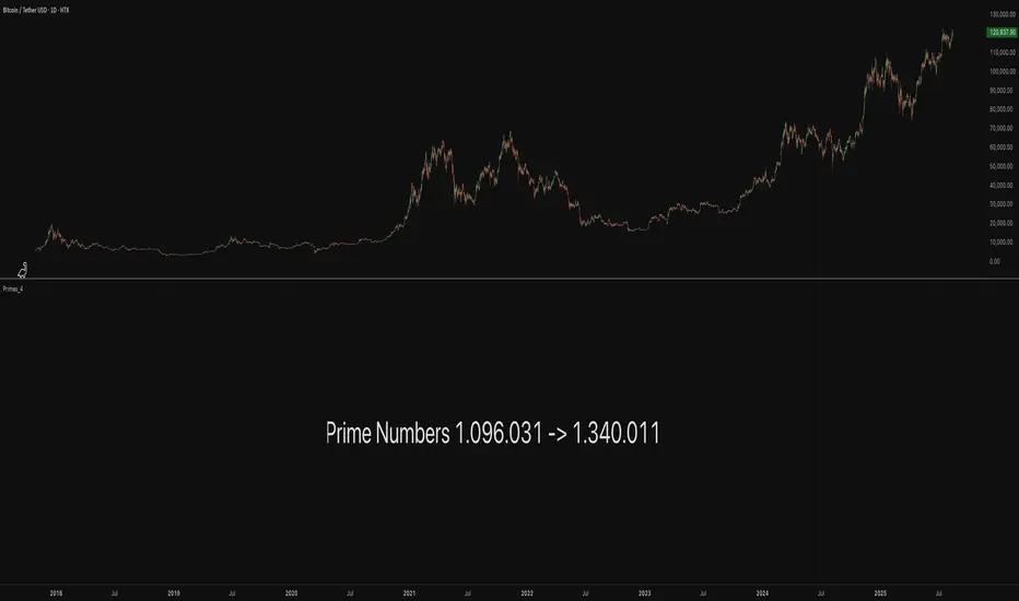
Primes_4These libraries (Primes_1 -> Primes_4) contain arrays of reduced Prime Numbers to minimize the amount of tokens, allowing more information to be exported.
Values, for example:
7001, 7013, 7019, 7027, 7039, 7043, 7057, 7069, 7079, 7103, 7109, 7021
are reduced to:
7001, 13, 19, 27, 39, 43, 57, 69, 79, 7103, 9, 21
With the restoreValues() function found in this library, the reduced values can be restored back to its original state.
7001, 13, 19, 27, 39, 43, 57, 69, 79, 7103, 9, 21
is restored back to:
7001, 7013, 7019, 7027, 7039, 7043, 7057, 7069, 7079, 7103, 7109, 7021
The libraries contain all Prime Numbers from 2 to 1.340.011
------------------------------------------------------------
Library "Primes_4"
Prime Numbers 1.096.031 - 1.340.011
primes_a()
Prime numbers 1.096.031 - 1.205.999
primes_b()
Prime numbers 1.206.013 - 1.317.989
primes_c()
Prime numbers 1.318.003 - 1.340.011
method restoreValues(iArray, iShow, iFrom, iTo)
restoreValues : Restores reduced prime number values in an array to their original state, for example `7001, 13, 19, 27, 39, 43, 57, 69, 79, 7103, 9, 21` is restored to `7001, 7013, 7019, 7027, 7039, 7043, 7057, 7069, 7079, 7103, 7109, 7021`
Namespace types: array
Parameters:
iArray (array)
iShow (bool)
iFrom (int)
iTo (int)
Returns: Initial array with restored prime number values
Ratio-Adjusted McClellan Summation Index RASI NASIRatio-Adjusted McClellan Summation Index (RASI NASI)
In Book "The Complete Guide to Market Breadth Indicators" Author Gregory L. Morris states
"It is the author’s opinion that the McClellan indicators, and in particular, the McClellan Summation Index, is the single best breadth indicator available. If you had to pick just one, this would be it."
What It Does: The Ratio-Adjusted McClellan Summation Index (RASI) is a market breadth indicator that tracks the cumulative strength of advancing versus declining issues for a user-selected exchange (NASDAQ, NYSE, or AMEX). Derived from the McClellan Oscillator, it calculates ratio-adjusted net advances, applies 19-day and 39-day EMAs, and sums the oscillator values to produce the RASI. This indicator helps traders assess market health, identify bullish or bearish trends, and detect potential reversals through divergences.
Key features:
Exchange Selection : Choose NASDAQ (USI:ADVN.NQ, USI:DECL.NQ), NYSE (USI:ADVN.NY, USI:DECL.NY), or AMEX (USI:ADVN.AM, USI:DECL.AM) data.
Trend-Based Coloring : RASI line displays user-defined colors (default: black for uptrend, red for downtrend) based on its direction.
Customizable Moving Average: Add a moving average (SMA, EMA, WMA, VWMA, or RMA) with user-defined length and color (default: EMA, 21, green).
Neutral Line at Zero: Marks the neutral level for trend interpretation.
Alerts: Six custom alert conditions for trend changes, MA crosses, and zero-line crosses.
How to Use
Add to Chart: Apply the indicator to any TradingView chart. Ensure access to advancing and declining issues data for the selected exchange.
Select Exchange: Choose NASDAQ, NYSE, or AMEX in the input settings.
Customize Settings: Adjust EMA lengths, RASI colors, MA type, length, and color to match your trading style.
Interpret the Indicator :
RASI Line: Black (default) indicates an uptrend (RASI rising); red indicates a downtrend (RASI falling).
Above Zero: Suggests bullish market breadth (more advancing issues).
Below Zero : Indicates bearish breadth (more declining issues).
MA Crosses: RASI crossing above its MA signals bullish momentum; crossing below signals bearish momentum.
Divergences: Compare RASI with the market index (e.g., NASDAQ Composite) to identify potential reversals.
Large Moves : A +3,600-point move from a low (e.g., -1,550 to +1,950) may signal a significant bull run.
Set Alerts:
Add the indicator to your chart, open the TradingView alert panel, and select from six conditions (see Alerts section).
Configure notifications (e.g., email, webhook, or popup) for each condition.
Settings
Market Selection:
Exchange: Select NASDAQ, NYSE, or AMEX for advancing/declining issues data.
EMA Settings:
19-day EMA Length: Period for the shorter EMA (default: 19).
39-day EMA Length: Period for the longer EMA (default: 39).
RASI Settings:
RASI Uptrend Color: Color for rising RASI (default: black).
RASI Downtrend Color: Color for falling RASI (default: red).
RASI MA Settings:
MA Type: Choose SMA, EMA, WMA, VWMA, or RMA (default: EMA).
MA Length: Set the MA period (default: 21).
MA Color: Color for the MA line (default: green).
Alerts
The indicator uses alertcondition() to create custom alerts. Available conditions:
RASI Trend Up: RASI starts rising (based on RASI > previous RASI, shown as black line).
RASI Trend Down: RASI starts falling (based on RASI ≤ previous RASI, shown as red line).
RASI Above MA: RASI crosses above its moving average.
RASI Below MA: RASI crosses below its moving average.
RASI Bullish: RASI crosses above zero (bullish market breadth).
RASI Bearish: RASI crosses below zero (bearish market breadth).
To set alerts, add the indicator to your chart, open the TradingView alert panel, and select the desired condition.
Notes
Data Requirements: Requires access to advancing/declining issues data (e.g., USI:ADVN.NQ, USI:DECL.NQ for NASDAQ). Some symbols may require a TradingView premium subscription.
Limitations: RASI is a medium- to long-term indicator and may lag in volatile or range-bound markets. Use alongside other technical tools for confirmation.
Data Reliability : Verify the selected exchange’s data accuracy, as inconsistencies can affect results.
Debugging: If no data appears, check symbol validity (e.g., try $ADVN/Q, $DECN/Q for NASDAQ) or contact TradingView support.
Credits
Based on the Ratio-Adjusted McClellan Summation Index methodology by McClellan Financial Publications. No external code was used; the implementation is original, inspired by standard market breadth concepts.
Disclaimer
This indicator is for informational purposes only and does not constitute financial advice. Past performance is not indicative of future results. Conduct your own research and combine with other tools for informed trading decisions.

Multi-Session ORBThe Multi-Session ORB Indicator is a customizable Pine Script (version 6) tool designed for TradingView to plot Opening Range Breakout (ORB) levels across four major trading sessions: Sydney, Tokyo, London, and New York. It allows traders to define specific ORB durations and session times in Central Daylight Time (CDT), making it adaptable to various trading strategies.
Key Features:
1. Customizable ORB Duration: Users can set the ORB duration (default: 15 minutes) via the inputMax parameter, determining the time window for calculating the high and low of each session’s opening range.
2. Flexible Session Times: The indicator supports user-defined session and ORB times for:
◦ Sydney: Default ORB (17:00–17:15 CDT), Session (17:00–01:00 CDT)
◦ Tokyo: Default ORB (19:00–19:15 CDT), Session (19:00–04:00 CDT)
◦ London: Default ORB (02:00–02:15 CDT), Session (02:00–11:00 CDT)
◦ New York: Default ORB (08:30–08:45 CDT), Session (08:30–16:00 CDT)
3. Session-Specific ORB Levels: For each session, the indicator calculates and tracks the high and low prices during the specified ORB period. These levels are updated dynamically if new highs or lows occur within the ORB timeframe.
4. Visual Representation:
◦ ORB high and low lines are plotted only during their respective session times, ensuring clarity.
◦ Each session’s lines are color-coded for easy identification:
▪ Sydney: Light Yellow (high), Dark Yellow (low)
▪ Tokyo: Light Pink (high), Dark Pink (low)
▪ London: Light Blue (high), Dark Blue (low)
▪ New York: Light Purple (high), Dark Purple (low)
◦ Lines are drawn with a linewidth of 2 and disappear when the session ends or if the timeframe is not intraday (or exceeds the ORB duration).
5. Intraday Compatibility: The indicator is optimized for intraday timeframes (e.g., 1-minute to 15-minute charts) and only displays when the chart’s timeframe multiplier is less than or equal to the ORB duration.
How It Works:
• Session Detection: The script uses the time() function to check if the current bar falls within the user-defined ORB or session time windows, accounting for all days of the week.
• ORB Logic: At the start of each session’s ORB period, the script initializes the high and low based on the first bar’s prices. It then updates these levels if subsequent bars within the ORB period exceed the current high or fall below the current low.
• Plotting: ORB levels are plotted as horizontal lines during the respective session, with visibility controlled to avoid clutter outside session times or on incompatible timeframes.
Use Case:
Traders can use this indicator to identify key breakout levels for each trading session, facilitating strategies based on price action around the opening range. The flexibility to adjust ORB and session times makes it suitable for various markets (e.g., forex, stocks, or futures) and time zones.
Limitations:
• The indicator is designed for intraday timeframes and may not display on higher timeframes (e.g., daily or weekly) or if the timeframe multiplier exceeds the ORB duration.
• Time inputs are in CDT, requiring users to adjust for their local timezone or market requirements.
• If you need to use this for GC/CL/SPY/QQQ you have to adjust the times by one hour.
This indicator is ideal for traders focusing on session-based breakout strategies, offering clear visualization and customization for global market sessions.

[GYTS] FiltersToolkit LibraryFiltersToolkit Library
🌸 Part of GoemonYae Trading System (GYTS) 🌸
🌸 --------- 1. INTRODUCTION --------- 🌸
💮 What Does This Library Contain?
This library is a curated collection of high-performance digital signal processing (DSP) filters and auxiliary functions designed specifically for financial time series analysis. It includes a shortlist of our favourite and best performing filters — each rigorously tested and selected for their responsiveness, minimal lag and robustness in diverse market conditions. These tools form an integral part of the GoemonYae Trading System (GYTS), chosen for their unique characteristics in handling market data.
The library contains two main categories:
1. Smoothing filters (low-pass filters and moving averages) for e.g. denoising, trend following
2. Detrending tools (high-pass and band-pass filters, known as "oscillators") for e.g. mean reversion
This collection is finely tuned for practical trading applications and is therefore not meant to be exhaustive. However, will continue to expand as we discover and validate new filtering techniques. I welcome collaboration and suggestions for novel approaches.
🌸 ——— 2. ADDED VALUE ——— 🌸
💮 Unified syntax and comprehensive documentation
The FiltersToolkit Library brings together a wide array of valuable filters under a unified, intuitive syntax. Each function is thoroughly documented, with clear explanations and academic sources that underline the mathematical rigour behind the methods. This level of documentation not only facilitates integration into trading strategies but also helps underlying the underlying concepts and rationale.
💮 Optimised performance and readability
The code prioritizes computational efficiency while maintaining readability. Key optimizations include:
- Minimizing redundant calculations in recursive filters
- Smart coefficient caching
- Efficient state management
- Vectorized operations where applicable
💮 Enhanced functionality and flexibility
Some filters in this library introduce extended functionality beyond the original publications. For instance, the MESA Adaptive Moving Average (MAMA) and Ehlers’ Combined Bandpass Filter incorporate multiple variations found in the literature, thereby providing traders with flexible tools that can be fine-tuned to different market conditions.
🌸 ——— 3. THE FILTERS ——— 🌸
💮 Hilbert Transform Function
This function implements the Hilbert Transform as utilised by John Ehlers. It converts a real-valued time series into its analytic signal, enabling the extraction of instantaneous phase and frequency information—an essential step in adaptive filtering.
Source: John Ehlers - "Rocket Science for Traders" (2001), "TASC 2001 V. 19:9", "Cybernetic Analysis for Stocks and Futures" (2004)
💮 Homodyne Discriminator
By leveraging the Hilbert Transform, this function computes the dominant cycle period through a Homodyne Discriminator. It extracts the in-phase and quadrature components of the signal, facilitating a robust estimation of the underlying cycle characteristics.
Source: John Ehlers - "Rocket Science for Traders" (2001), "TASC 2001 V. 19:9", "Cybernetic Analysis for Stocks and Futures" (2004)
💮 MESA Adaptive Moving Average (MAMA)
An advanced dual-stage adaptive moving average, this function outputs both the MAMA and its companion FAMA. It combines adaptive alpha computation with elements from Kaufman’s Adaptive Moving Average (KAMA) to provide a responsive and reliable trend indicator.
Source: John Ehlers - "Rocket Science for Traders" (2001), "TASC 2001 V. 19:9", "Cybernetic Analysis for Stocks and Futures" (2004)
💮 BiQuad Filters
A family of second-order recursive filters offering exceptional control over frequency response:
- High-pass filter for detrending
- Low-pass filter for smooth trend following
- Band-pass filter for cycle isolation
The quality factor (Q) parameter allows fine-tuning of the resonance characteristics, making these filters highly adaptable to different market conditions.
Source: Robert Bristow-Johnson's Audio EQ Cookbook, implemented by @The_Peaceful_Lizard
💮 Relative Vigor Index (RVI)
This filter evaluates the strength of a trend by comparing the closing price to the trading range. Operating similarly to a band-pass filter, the RVI provides insights into market momentum and potential reversals.
Source: John Ehlers – “Cybernetic Analysis for Stocks and Futures” (2004)
💮 Cyber Cycle
The Cyber Cycle filter emphasises market cycles by smoothing out noise and highlighting the dominant cyclical behaviour. It is particularly useful for detecting trend reversals and cyclical patterns in the price data.
Source: John Ehlers – “Cybernetic Analysis for Stocks and Futures” (2004)
💮 Butterworth High Pass Filter
Inspired by the classical Butterworth design, this filter achieves a maximally flat magnitude response in the passband while effectively removing low-frequency trends. Its design minimises phase distortion, which is vital for accurate signal interpretation.
Source: John Ehlers – “Cybernetic Analysis for Stocks and Futures” (2004)
💮 2-Pole SuperSmoother
Employing a two-pole design, the SuperSmoother filter reduces high-frequency noise with minimal lag. It is engineered to preserve trend integrity while offering a smooth output even in noisy market conditions.
Source: John Ehlers – “Cybernetic Analysis for Stocks and Futures” (2004)
💮 3-Pole SuperSmoother
An extension of the 2-pole design, the 3-pole SuperSmoother further attenuates high-frequency noise. Its additional pole delivers enhanced smoothing at the cost of slightly increased lag.
Source: John Ehlers – “Cybernetic Analysis for Stocks and Futures” (2004)
💮 Adaptive Directional Volatility Moving Average (ADXVma)
This adaptive moving average adjusts its smoothing factor based on directional volatility. By combining true range and directional movement measurements, it remains exceptionally flat during ranging markets and responsive during directional moves.
Source: Various implementations across platforms, unified and optimized
💮 Ehlers Combined Bandpass Filter with Automated Gain Control (AGC)
This sophisticated filter merges a highpass pre-processing stage with a bandpass filter. An integrated Automated Gain Control normalises the output to a consistent range, while offering both regular and truncated recursive formulations to manage lag.
Source: John F. Ehlers – “Truncated Indicators” (2020), “Cycle Analytics for Traders” (2013)
💮 Voss Predictive Filter
A forward-looking filter that predicts future values of a band-limited signal in real time. By utilising multiple time-delayed feedback terms, it provides anticipatory coupling and delivers a short-term predictive signal.
Source: John Ehlers - "A Peek Into The Future" (TASC 2019-08)
💮 Adaptive Autonomous Recursive Moving Average (A2RMA)
This filter dynamically adjusts its smoothing through an adaptive mechanism based on an efficiency ratio and a dynamic threshold. A double application of an adaptive moving average ensures both responsiveness and stability in volatile and ranging markets alike. Very flat response when properly tuned.
Source: @alexgrover (2019)
💮 Ultimate Smoother (2-Pole)
The Ultimate Smoother filter is engineered to achieve near-zero lag in its passband by subtracting a high-pass response from an all-pass response. This creates a filter that maintains signal fidelity at low frequencies while effectively filtering higher frequencies at the expense of slight overshooting.
Source: John Ehlers - TASC 2024-04 "The Ultimate Smoother"
Note: This library is actively maintained and enhanced. Suggestions for additional filters or improvements are welcome through the usual channels. The source code contains a list of tested filters that did not make it into the curated collection.
Universal Ratio Trend Matrix [InvestorUnknown]The Universal Ratio Trend Matrix is designed for trend analysis on asset/asset ratios, supporting up to 40 different assets. Its primary purpose is to help identify which assets are outperforming others within a selection, providing a broad overview of market trends through a matrix of ratios. The indicator automatically expands the matrix based on the number of assets chosen, simplifying the process of comparing multiple assets in terms of performance.
Key features include the ability to choose from a narrow selection of indicators to perform the ratio trend analysis, allowing users to apply well-defined metrics to their comparison.
Drawback: Due to the computational intensity involved in calculating ratios across many assets, the indicator has a limitation related to loading speed. TradingView has time limits for calculations, and for users on the basic (free) plan, this could result in frequent errors due to exceeded time limits. To use the indicator effectively, users with any paid plans should run it on timeframes higher than 8h (the lowest timeframe on which it managed to load with 40 assets), as lower timeframes may not reliably load.
Indicators:
RSI_raw: Simple function to calculate the Relative Strength Index (RSI) of a source (asset price).
RSI_sma: Calculates RSI followed by a Simple Moving Average (SMA).
RSI_ema: Calculates RSI followed by an Exponential Moving Average (EMA).
CCI: Calculates the Commodity Channel Index (CCI).
Fisher: Implements the Fisher Transform to normalize prices.
Utility Functions:
f_remove_exchange_name: Strips the exchange name from asset tickers (e.g., "INDEX:BTCUSD" to "BTCUSD").
f_remove_exchange_name(simple string name) =>
string parts = str.split(name, ":")
string result = array.size(parts) > 1 ? array.get(parts, 1) : name
result
f_get_price: Retrieves the closing price of a given asset ticker using request.security().
f_constant_src: Checks if the source data is constant by comparing multiple consecutive values.
Inputs:
General settings allow users to select the number of tickers for analysis (used_assets) and choose the trend indicator (RSI, CCI, Fisher, etc.).
Table settings customize how trend scores are displayed in terms of text size, header visibility, highlighting options, and top-performing asset identification.
The script includes inputs for up to 40 assets, allowing the user to select various cryptocurrencies (e.g., BTCUSD, ETHUSD, SOLUSD) or other assets for trend analysis.
Price Arrays:
Price values for each asset are stored in variables (price_a1 to price_a40) initialized as na. These prices are updated only for the number of assets specified by the user (used_assets).
Trend scores for each asset are stored in separate arrays
// declare price variables as "na"
var float price_a1 = na, var float price_a2 = na, var float price_a3 = na, var float price_a4 = na, var float price_a5 = na
var float price_a6 = na, var float price_a7 = na, var float price_a8 = na, var float price_a9 = na, var float price_a10 = na
var float price_a11 = na, var float price_a12 = na, var float price_a13 = na, var float price_a14 = na, var float price_a15 = na
var float price_a16 = na, var float price_a17 = na, var float price_a18 = na, var float price_a19 = na, var float price_a20 = na
var float price_a21 = na, var float price_a22 = na, var float price_a23 = na, var float price_a24 = na, var float price_a25 = na
var float price_a26 = na, var float price_a27 = na, var float price_a28 = na, var float price_a29 = na, var float price_a30 = na
var float price_a31 = na, var float price_a32 = na, var float price_a33 = na, var float price_a34 = na, var float price_a35 = na
var float price_a36 = na, var float price_a37 = na, var float price_a38 = na, var float price_a39 = na, var float price_a40 = na
// create "empty" arrays to store trend scores
var a1_array = array.new_int(40, 0), var a2_array = array.new_int(40, 0), var a3_array = array.new_int(40, 0), var a4_array = array.new_int(40, 0)
var a5_array = array.new_int(40, 0), var a6_array = array.new_int(40, 0), var a7_array = array.new_int(40, 0), var a8_array = array.new_int(40, 0)
var a9_array = array.new_int(40, 0), var a10_array = array.new_int(40, 0), var a11_array = array.new_int(40, 0), var a12_array = array.new_int(40, 0)
var a13_array = array.new_int(40, 0), var a14_array = array.new_int(40, 0), var a15_array = array.new_int(40, 0), var a16_array = array.new_int(40, 0)
var a17_array = array.new_int(40, 0), var a18_array = array.new_int(40, 0), var a19_array = array.new_int(40, 0), var a20_array = array.new_int(40, 0)
var a21_array = array.new_int(40, 0), var a22_array = array.new_int(40, 0), var a23_array = array.new_int(40, 0), var a24_array = array.new_int(40, 0)
var a25_array = array.new_int(40, 0), var a26_array = array.new_int(40, 0), var a27_array = array.new_int(40, 0), var a28_array = array.new_int(40, 0)
var a29_array = array.new_int(40, 0), var a30_array = array.new_int(40, 0), var a31_array = array.new_int(40, 0), var a32_array = array.new_int(40, 0)
var a33_array = array.new_int(40, 0), var a34_array = array.new_int(40, 0), var a35_array = array.new_int(40, 0), var a36_array = array.new_int(40, 0)
var a37_array = array.new_int(40, 0), var a38_array = array.new_int(40, 0), var a39_array = array.new_int(40, 0), var a40_array = array.new_int(40, 0)
f_get_price(simple string ticker) =>
request.security(ticker, "", close)
// Prices for each USED asset
f_get_asset_price(asset_number, ticker) =>
if (used_assets >= asset_number)
f_get_price(ticker)
else
na
// overwrite empty variables with the prices if "used_assets" is greater or equal to the asset number
if barstate.isconfirmed // use barstate.isconfirmed to avoid "na prices" and calculation errors that result in empty cells in the table
price_a1 := f_get_asset_price(1, asset1), price_a2 := f_get_asset_price(2, asset2), price_a3 := f_get_asset_price(3, asset3), price_a4 := f_get_asset_price(4, asset4)
price_a5 := f_get_asset_price(5, asset5), price_a6 := f_get_asset_price(6, asset6), price_a7 := f_get_asset_price(7, asset7), price_a8 := f_get_asset_price(8, asset8)
price_a9 := f_get_asset_price(9, asset9), price_a10 := f_get_asset_price(10, asset10), price_a11 := f_get_asset_price(11, asset11), price_a12 := f_get_asset_price(12, asset12)
price_a13 := f_get_asset_price(13, asset13), price_a14 := f_get_asset_price(14, asset14), price_a15 := f_get_asset_price(15, asset15), price_a16 := f_get_asset_price(16, asset16)
price_a17 := f_get_asset_price(17, asset17), price_a18 := f_get_asset_price(18, asset18), price_a19 := f_get_asset_price(19, asset19), price_a20 := f_get_asset_price(20, asset20)
price_a21 := f_get_asset_price(21, asset21), price_a22 := f_get_asset_price(22, asset22), price_a23 := f_get_asset_price(23, asset23), price_a24 := f_get_asset_price(24, asset24)
price_a25 := f_get_asset_price(25, asset25), price_a26 := f_get_asset_price(26, asset26), price_a27 := f_get_asset_price(27, asset27), price_a28 := f_get_asset_price(28, asset28)
price_a29 := f_get_asset_price(29, asset29), price_a30 := f_get_asset_price(30, asset30), price_a31 := f_get_asset_price(31, asset31), price_a32 := f_get_asset_price(32, asset32)
price_a33 := f_get_asset_price(33, asset33), price_a34 := f_get_asset_price(34, asset34), price_a35 := f_get_asset_price(35, asset35), price_a36 := f_get_asset_price(36, asset36)
price_a37 := f_get_asset_price(37, asset37), price_a38 := f_get_asset_price(38, asset38), price_a39 := f_get_asset_price(39, asset39), price_a40 := f_get_asset_price(40, asset40)
Universal Indicator Calculation (f_calc_score):
This function allows switching between different trend indicators (RSI, CCI, Fisher) for flexibility.
It uses a switch-case structure to calculate the indicator score, where a positive trend is denoted by 1 and a negative trend by 0. Each indicator has its own logic to determine whether the asset is trending up or down.
// use switch to allow "universality" in indicator selection
f_calc_score(source, trend_indicator, int_1, int_2) =>
int score = na
if (not f_constant_src(source)) and source > 0.0 // Skip if you are using the same assets for ratio (for example BTC/BTC)
x = switch trend_indicator
"RSI (Raw)" => RSI_raw(source, int_1)
"RSI (SMA)" => RSI_sma(source, int_1, int_2)
"RSI (EMA)" => RSI_ema(source, int_1, int_2)
"CCI" => CCI(source, int_1)
"Fisher" => Fisher(source, int_1)
y = switch trend_indicator
"RSI (Raw)" => x > 50 ? 1 : 0
"RSI (SMA)" => x > 50 ? 1 : 0
"RSI (EMA)" => x > 50 ? 1 : 0
"CCI" => x > 0 ? 1 : 0
"Fisher" => x > x ? 1 : 0
score := y
else
score := 0
score
Array Setting Function (f_array_set):
This function populates an array with scores calculated for each asset based on a base price (p_base) divided by the prices of the individual assets.
It processes multiple assets (up to 40), calling the f_calc_score function for each.
// function to set values into the arrays
f_array_set(a_array, p_base) =>
array.set(a_array, 0, f_calc_score(p_base / price_a1, trend_indicator, int_1, int_2))
array.set(a_array, 1, f_calc_score(p_base / price_a2, trend_indicator, int_1, int_2))
array.set(a_array, 2, f_calc_score(p_base / price_a3, trend_indicator, int_1, int_2))
array.set(a_array, 3, f_calc_score(p_base / price_a4, trend_indicator, int_1, int_2))
array.set(a_array, 4, f_calc_score(p_base / price_a5, trend_indicator, int_1, int_2))
array.set(a_array, 5, f_calc_score(p_base / price_a6, trend_indicator, int_1, int_2))
array.set(a_array, 6, f_calc_score(p_base / price_a7, trend_indicator, int_1, int_2))
array.set(a_array, 7, f_calc_score(p_base / price_a8, trend_indicator, int_1, int_2))
array.set(a_array, 8, f_calc_score(p_base / price_a9, trend_indicator, int_1, int_2))
array.set(a_array, 9, f_calc_score(p_base / price_a10, trend_indicator, int_1, int_2))
array.set(a_array, 10, f_calc_score(p_base / price_a11, trend_indicator, int_1, int_2))
array.set(a_array, 11, f_calc_score(p_base / price_a12, trend_indicator, int_1, int_2))
array.set(a_array, 12, f_calc_score(p_base / price_a13, trend_indicator, int_1, int_2))
array.set(a_array, 13, f_calc_score(p_base / price_a14, trend_indicator, int_1, int_2))
array.set(a_array, 14, f_calc_score(p_base / price_a15, trend_indicator, int_1, int_2))
array.set(a_array, 15, f_calc_score(p_base / price_a16, trend_indicator, int_1, int_2))
array.set(a_array, 16, f_calc_score(p_base / price_a17, trend_indicator, int_1, int_2))
array.set(a_array, 17, f_calc_score(p_base / price_a18, trend_indicator, int_1, int_2))
array.set(a_array, 18, f_calc_score(p_base / price_a19, trend_indicator, int_1, int_2))
array.set(a_array, 19, f_calc_score(p_base / price_a20, trend_indicator, int_1, int_2))
array.set(a_array, 20, f_calc_score(p_base / price_a21, trend_indicator, int_1, int_2))
array.set(a_array, 21, f_calc_score(p_base / price_a22, trend_indicator, int_1, int_2))
array.set(a_array, 22, f_calc_score(p_base / price_a23, trend_indicator, int_1, int_2))
array.set(a_array, 23, f_calc_score(p_base / price_a24, trend_indicator, int_1, int_2))
array.set(a_array, 24, f_calc_score(p_base / price_a25, trend_indicator, int_1, int_2))
array.set(a_array, 25, f_calc_score(p_base / price_a26, trend_indicator, int_1, int_2))
array.set(a_array, 26, f_calc_score(p_base / price_a27, trend_indicator, int_1, int_2))
array.set(a_array, 27, f_calc_score(p_base / price_a28, trend_indicator, int_1, int_2))
array.set(a_array, 28, f_calc_score(p_base / price_a29, trend_indicator, int_1, int_2))
array.set(a_array, 29, f_calc_score(p_base / price_a30, trend_indicator, int_1, int_2))
array.set(a_array, 30, f_calc_score(p_base / price_a31, trend_indicator, int_1, int_2))
array.set(a_array, 31, f_calc_score(p_base / price_a32, trend_indicator, int_1, int_2))
array.set(a_array, 32, f_calc_score(p_base / price_a33, trend_indicator, int_1, int_2))
array.set(a_array, 33, f_calc_score(p_base / price_a34, trend_indicator, int_1, int_2))
array.set(a_array, 34, f_calc_score(p_base / price_a35, trend_indicator, int_1, int_2))
array.set(a_array, 35, f_calc_score(p_base / price_a36, trend_indicator, int_1, int_2))
array.set(a_array, 36, f_calc_score(p_base / price_a37, trend_indicator, int_1, int_2))
array.set(a_array, 37, f_calc_score(p_base / price_a38, trend_indicator, int_1, int_2))
array.set(a_array, 38, f_calc_score(p_base / price_a39, trend_indicator, int_1, int_2))
array.set(a_array, 39, f_calc_score(p_base / price_a40, trend_indicator, int_1, int_2))
a_array
Conditional Array Setting (f_arrayset):
This function checks if the number of used assets is greater than or equal to a specified number before populating the arrays.
// only set values into arrays for USED assets
f_arrayset(asset_number, a_array, p_base) =>
if (used_assets >= asset_number)
f_array_set(a_array, p_base)
else
na
Main Logic
The main logic initializes arrays to store scores for each asset. Each array corresponds to one asset's performance score.
Setting Trend Values: The code calls f_arrayset for each asset, populating the respective arrays with calculated scores based on the asset prices.
Combining Arrays: A combined_array is created to hold all the scores from individual asset arrays. This array facilitates further analysis, allowing for an overview of the performance scores of all assets at once.
// create a combined array (work-around since pinescript doesn't support having array of arrays)
var combined_array = array.new_int(40 * 40, 0)
if barstate.islast
for i = 0 to 39
array.set(combined_array, i, array.get(a1_array, i))
array.set(combined_array, i + (40 * 1), array.get(a2_array, i))
array.set(combined_array, i + (40 * 2), array.get(a3_array, i))
array.set(combined_array, i + (40 * 3), array.get(a4_array, i))
array.set(combined_array, i + (40 * 4), array.get(a5_array, i))
array.set(combined_array, i + (40 * 5), array.get(a6_array, i))
array.set(combined_array, i + (40 * 6), array.get(a7_array, i))
array.set(combined_array, i + (40 * 7), array.get(a8_array, i))
array.set(combined_array, i + (40 * 8), array.get(a9_array, i))
array.set(combined_array, i + (40 * 9), array.get(a10_array, i))
array.set(combined_array, i + (40 * 10), array.get(a11_array, i))
array.set(combined_array, i + (40 * 11), array.get(a12_array, i))
array.set(combined_array, i + (40 * 12), array.get(a13_array, i))
array.set(combined_array, i + (40 * 13), array.get(a14_array, i))
array.set(combined_array, i + (40 * 14), array.get(a15_array, i))
array.set(combined_array, i + (40 * 15), array.get(a16_array, i))
array.set(combined_array, i + (40 * 16), array.get(a17_array, i))
array.set(combined_array, i + (40 * 17), array.get(a18_array, i))
array.set(combined_array, i + (40 * 18), array.get(a19_array, i))
array.set(combined_array, i + (40 * 19), array.get(a20_array, i))
array.set(combined_array, i + (40 * 20), array.get(a21_array, i))
array.set(combined_array, i + (40 * 21), array.get(a22_array, i))
array.set(combined_array, i + (40 * 22), array.get(a23_array, i))
array.set(combined_array, i + (40 * 23), array.get(a24_array, i))
array.set(combined_array, i + (40 * 24), array.get(a25_array, i))
array.set(combined_array, i + (40 * 25), array.get(a26_array, i))
array.set(combined_array, i + (40 * 26), array.get(a27_array, i))
array.set(combined_array, i + (40 * 27), array.get(a28_array, i))
array.set(combined_array, i + (40 * 28), array.get(a29_array, i))
array.set(combined_array, i + (40 * 29), array.get(a30_array, i))
array.set(combined_array, i + (40 * 30), array.get(a31_array, i))
array.set(combined_array, i + (40 * 31), array.get(a32_array, i))
array.set(combined_array, i + (40 * 32), array.get(a33_array, i))
array.set(combined_array, i + (40 * 33), array.get(a34_array, i))
array.set(combined_array, i + (40 * 34), array.get(a35_array, i))
array.set(combined_array, i + (40 * 35), array.get(a36_array, i))
array.set(combined_array, i + (40 * 36), array.get(a37_array, i))
array.set(combined_array, i + (40 * 37), array.get(a38_array, i))
array.set(combined_array, i + (40 * 38), array.get(a39_array, i))
array.set(combined_array, i + (40 * 39), array.get(a40_array, i))
Calculating Sums: A separate array_sums is created to store the total score for each asset by summing the values of their respective score arrays. This allows for easy comparison of overall performance.
Ranking Assets: The final part of the code ranks the assets based on their total scores stored in array_sums. It assigns a rank to each asset, where the asset with the highest score receives the highest rank.
// create array for asset RANK based on array.sum
var ranks = array.new_int(used_assets, 0)
// for loop that calculates the rank of each asset
if barstate.islast
for i = 0 to (used_assets - 1)
int rank = 1
for x = 0 to (used_assets - 1)
if i != x
if array.get(array_sums, i) < array.get(array_sums, x)
rank := rank + 1
array.set(ranks, i, rank)
Dynamic Table Creation
Initialization: The table is initialized with a base structure that includes headers for asset names, scores, and ranks. The headers are set to remain constant, ensuring clarity for users as they interpret the displayed data.
Data Population: As scores are calculated for each asset, the corresponding values are dynamically inserted into the table. This is achieved through a loop that iterates over the scores and ranks stored in the combined_array and array_sums, respectively.
Automatic Extending Mechanism
Variable Asset Count: The code checks the number of assets defined by the user. Instead of hardcoding the number of rows in the table, it uses a variable to determine the extent of the data that needs to be displayed. This allows the table to expand or contract based on the number of assets being analyzed.
Dynamic Row Generation: Within the loop that populates the table, the code appends new rows for each asset based on the current asset count. The structure of each row includes the asset name, its score, and its rank, ensuring that the table remains consistent regardless of how many assets are involved.
// Automatically extending table based on the number of used assets
var table table = table.new(position.bottom_center, 50, 50, color.new(color.black, 100), color.white, 3, color.white, 1)
if barstate.islast
if not hide_head
table.cell(table, 0, 0, "Universal Ratio Trend Matrix", text_color = color.white, bgcolor = #010c3b, text_size = fontSize)
table.merge_cells(table, 0, 0, used_assets + 3, 0)
if not hide_inps
table.cell(table, 0, 1,
text = "Inputs: You are using " + str.tostring(trend_indicator) + ", which takes: " + str.tostring(f_get_input(trend_indicator)),
text_color = color.white, text_size = fontSize), table.merge_cells(table, 0, 1, used_assets + 3, 1)
table.cell(table, 0, 2, "Assets", text_color = color.white, text_size = fontSize, bgcolor = #010c3b)
for x = 0 to (used_assets - 1)
table.cell(table, x + 1, 2, text = str.tostring(array.get(assets, x)), text_color = color.white, bgcolor = #010c3b, text_size = fontSize)
table.cell(table, 0, x + 3, text = str.tostring(array.get(assets, x)), text_color = color.white, bgcolor = f_asset_col(array.get(ranks, x)), text_size = fontSize)
for r = 0 to (used_assets - 1)
for c = 0 to (used_assets - 1)
table.cell(table, c + 1, r + 3, text = str.tostring(array.get(combined_array, c + (r * 40))),
text_color = hl_type == "Text" ? f_get_col(array.get(combined_array, c + (r * 40))) : color.white, text_size = fontSize,
bgcolor = hl_type == "Background" ? f_get_col(array.get(combined_array, c + (r * 40))) : na)
for x = 0 to (used_assets - 1)
table.cell(table, x + 1, x + 3, "", bgcolor = #010c3b)
table.cell(table, used_assets + 1, 2, "", bgcolor = #010c3b)
for x = 0 to (used_assets - 1)
table.cell(table, used_assets + 1, x + 3, "==>", text_color = color.white)
table.cell(table, used_assets + 2, 2, "SUM", text_color = color.white, text_size = fontSize, bgcolor = #010c3b)
table.cell(table, used_assets + 3, 2, "RANK", text_color = color.white, text_size = fontSize, bgcolor = #010c3b)
for x = 0 to (used_assets - 1)
table.cell(table, used_assets + 2, x + 3,
text = str.tostring(array.get(array_sums, x)),
text_color = color.white, text_size = fontSize,
bgcolor = f_highlight_sum(array.get(array_sums, x), array.get(ranks, x)))
table.cell(table, used_assets + 3, x + 3,
text = str.tostring(array.get(ranks, x)),
text_color = color.white, text_size = fontSize,
bgcolor = f_highlight_rank(array.get(ranks, x)))

KillZones & Sessions [TradingFinder] Volume | Asia, London & NY🔵 Introduction
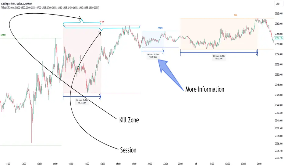
🟣 Session
The forex market operates 24 hours a day, 5 days a week, with only Saturdays and Sundays being off; traders often focus on one of the forex trading sessions instead of trying to trade in all markets 24 hours a day.
Trading sessions are time intervals during which a specific financial market is active and trades are conducted. The Asia, London, and New York sessions are the most important trading sessions throughout the 24-hour period, during which a significant amount of money and liquidity enters the market.
🟣 Kill Zone
Traders in financial markets profit from the difference between the price at which they buy or sell and the current market price. Traders have different time horizons for trading.
Among these, some traders engage in daily or even hourly trading and must operate during times when the market has desirable trading volumes and significant price movements.
Kill zones are segments of a session with higher trading volumes and price fluctuations compared to the rest of the session.
🔵 How to Use
🟣 Session Time
The "Asia Session" consists of two sessions: "Sydney" and "Tokyo." The beginning of this session, according to the "UTC" time zone, is at 23:00 and ends at 06:00. Similarly, the beginning of the "Asia KillZone," according to the "UTC" time zone, is at 23:00, and it ends at 03:55.
The "London Session" consists of two sessions: "Frankfurt" and "London." The beginning of this session, according to the "UTC" time zone, is at 07:00, and it ends at 14:25. Similarly, the beginning of the "London KillZone," according to the "UTC" time zone, is at 07:00, and it ends at 09:55.
The beginning of the "New York am" session, according to the "UTC" time zone, is at 14:30, and it ends at 19:25. Similarly, the beginning of the "New York am KillZone," according to the "UTC" time zone, is at 14:30, and it ends at 16:55.
The beginning of the "New York pm" session, according to the "UTC" time zone, is at 19:30, and it ends at 22:55. Similarly, the beginning of the "New York pm KillZone," according to the "UTC" time zone, is at 19:30, and it ends at 20:55.
Important : To prevent session overlap, the working hours of each session have slightly changed.
🔵 Features
🟣 Simultaneous Session and Kill Zone
With this indicator, you can simultaneously view the kill zone and session. High and low lines are used to indicate sessions, while filled areas with color represent kill zones. If you do not want to see kill zones, you can turn off the display settings.
🟣 Candle, Time, and Volume
Using the "More Info" feature, you can see the number of candles, elapsed time, and traded volume within the colored filled area.
🔵 Settings
•Show More Info: To display "More Info," you need to turn on this feature and turn it off whenever you don't need it.
• You can also customize these settings for each session separately :
o Display or hide session.
o Choose session color.
o Set session time range.
o Display or hide kill zone.
o Set kill zone time range.
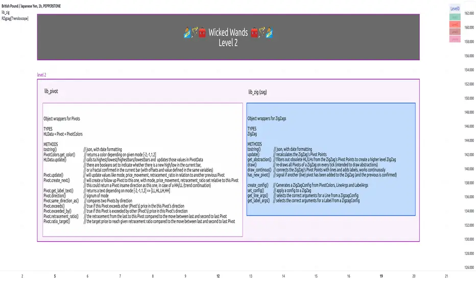
lib_zigLibrary "lib_zig"
Object oriented implementation of ZigZag
method tostring(this, date_format)
Namespace types: Zigzag
Parameters:
this (Zigzag)
date_format (simple string)
method update(this)
Namespace types: Zigzag
Parameters:
this (Zigzag)
method draw(this, colors)
Namespace types: Zigzag
Parameters:
this (Zigzag)
colors (PivotColors type from robbatt/lib_pivot/19)
Zigzag
Fields:
max_pivots (series__integer)
hldata (|robbatt/lib_pivot/19;HLData|#OBJ)
pivots (array__|robbatt/lib_pivot/19;Pivot|#OBJ)
CDC ActionZone BF for ETHUSD-1D © PRoSkYNeT-EE
Based on improvements from "Kitti-Playbook Action Zone V.4.2.0.3 for Stock Market"
Based on improvements from "CDC Action Zone V3 2020 by piriya33"
Based on Triple MACD crossover between 9/15, 21/28, 15/28 for filter error signal (noise) from CDC ActionZone V3
MACDs generated from the execution of millions of times in the "Brute Force Algorithm" to backtest data from the past 5 years. ( 2017-08-21 to 2022-08-01 )
Released 2022-08-01
***** The indicator is used in the ETHUSD 1 Day period ONLY *****
Recommended Stop Loss : -4 % (execute stop Loss after candlestick has been closed)
Backtest Result ( Start $100 )
Winrate 63 % (Win:12, Loss:7, Total:19)
Live Days 1,806 days
B : Buy
S : Sell
SL : Stop Loss
2022-07-19 07 - 1,542 : B 6.971 ETH
2022-04-13 07 - 3,118 : S 8.98 % $10,750 12,7,19 63 %
2022-03-20 07 - 2,861 : B 3.448 ETH
2021-12-03 07 - 4,216 : SL -8.94 % $9,864 11,7,18 61 %
2021-11-30 07 - 4,630 : B 2.340 ETH
2021-11-18 07 - 3,997 : S 13.71 % $10,832 11,6,17 65 %
2021-10-05 07 - 3,515 : B 2.710 ETH
2021-09-20 07 - 2,977 : S 29.38 % $9,526 10,6,16 63 %
2021-07-28 07 - 2,301 : B 3.200 ETH
2021-05-20 07 - 2,769 : S 50.49 % $7,363 9,6,15 60 %
2021-03-30 07 - 1,840 : B 2.659 ETH
2021-03-22 07 - 1,681 : SL -8.29 % $4,893 8,6,14 57 %
2021-03-08 07 - 1,833 : B 2.911 ETH
2021-02-26 07 - 1,445 : S 279.27 % $5,335 8,5,13 62 %
2020-10-13 07 - 381 : B 3.692 ETH
2020-09-05 07 - 335 : S 38.43 % $1,407 7,5,12 58 %
2020-07-06 07 - 242 : B 4.199 ETH
2020-06-27 07 - 221 : S 28.49 % $1,016 6,5,11 55 %
2020-04-16 07 - 172 : B 4.598 ETH
2020-02-29 07 - 217 : S 47.62 % $791 5,5,10 50 %
2020-01-12 07 - 147 : B 3.644 ETH
2019-11-18 07 - 178 : S -2.73 % $536 4,5,9 44 %
2019-11-01 07 - 183 : B 3.010 ETH
2019-09-23 07 - 201 : SL -4.29 % $551 4,4,8 50 %
2019-09-18 07 - 210 : B 2.740 ETH
2019-07-12 07 - 275 : S 63.69 % $575 4,3,7 57 %
2019-05-03 07 - 168 : B 2.093 ETH
2019-04-28 07 - 158 : S 29.51 % $352 3,3,6 50 %
2019-02-15 07 - 122 : B 2.225 ETH
2019-01-10 07 - 125 : SL -6.02 % $271 2,3,5 40 %
2018-12-29 07 - 133 : B 2.172 ETH
2018-05-22 07 - 641 : S 5.95 % $289 2,2,4 50 %
2018-04-21 07 - 605 : B 0.451 ETH
2018-02-02 07 - 922 : S 197.42 % $273 1,2,3 33 %
2017-11-11 07 - 310 : B 0.296 ETH
2017-10-09 07 - 297 : SL -4.50 % $92 0,2,2 0 %
2017-10-07 07 - 311 : B 0.309 ETH
2017-08-22 07 - 310 : SL -4.02 % $96 0,1,1 0 %
2017-08-21 07 - 323 : B 0.310 ETH
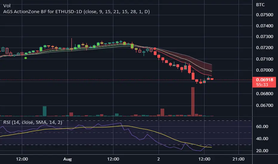
Quantum Rotational Field MappingQuantum Rotational Field Mapping (QRFM):
Phase Coherence Detection Through Complex-Plane Oscillator Analysis
Quantum Rotational Field Mapping applies complex-plane mathematics and phase-space analysis to oscillator ensembles, identifying high-probability trend ignition points by measuring when multiple independent oscillators achieve phase coherence. Unlike traditional multi-oscillator approaches that simply stack indicators or use boolean AND/OR logic, this system converts each oscillator into a rotating phasor (vector) in the complex plane and calculates the Coherence Index (CI) —a mathematical measure of how tightly aligned the ensemble has become—then generates signals only when alignment, phase direction, and pairwise entanglement all converge.
The indicator combines three mathematical frameworks: phasor representation using analytic signal theory to extract phase and amplitude from each oscillator, coherence measurement using vector summation in the complex plane to quantify group alignment, and entanglement analysis that calculates pairwise phase agreement across all oscillator combinations. This creates a multi-dimensional confirmation system that distinguishes between random oscillator noise and genuine regime transitions.
What Makes This Original
Complex-Plane Phasor Framework
This indicator implements classical signal processing mathematics adapted for market oscillators. Each oscillator—whether RSI, MACD, Stochastic, CCI, Williams %R, MFI, ROC, or TSI—is first normalized to a common scale, then converted into a complex-plane representation using an in-phase (I) and quadrature (Q) component. The in-phase component is the oscillator value itself, while the quadrature component is calculated as the first difference (derivative proxy), creating a velocity-aware representation.
From these components, the system extracts:
Phase (φ) : Calculated as φ = atan2(Q, I), representing the oscillator's position in its cycle (mapped to -180° to +180°)
Amplitude (A) : Calculated as A = √(I² + Q²), representing the oscillator's strength or conviction
This mathematical approach is fundamentally different from simply reading oscillator values. A phasor captures both where an oscillator is in its cycle (phase angle) and how strongly it's expressing that position (amplitude). Two oscillators can have the same value but be in opposite phases of their cycles—traditional analysis would see them as identical, while QRFM sees them as 180° out of phase (contradictory).
Coherence Index Calculation
The core innovation is the Coherence Index (CI) , borrowed from physics and signal processing. When you have N oscillators, each with phase φₙ, you can represent each as a unit vector in the complex plane: e^(iφₙ) = cos(φₙ) + i·sin(φₙ).
The CI measures what happens when you sum all these vectors:
Resultant Vector : R = Σ e^(iφₙ) = Σ cos(φₙ) + i·Σ sin(φₙ)
Coherence Index : CI = |R| / N
Where |R| is the magnitude of the resultant vector and N is the number of active oscillators.
The CI ranges from 0 to 1:
CI = 1.0 : Perfect coherence—all oscillators have identical phase angles, vectors point in the same direction, creating maximum constructive interference
CI = 0.0 : Complete decoherence—oscillators are randomly distributed around the circle, vectors cancel out through destructive interference
0 < CI < 1 : Partial alignment—some clustering with some scatter
This is not a simple average or correlation. The CI captures phase synchronization across the entire ensemble simultaneously. When oscillators phase-lock (align their cycles), the CI spikes regardless of their individual values. This makes it sensitive to regime transitions that traditional indicators miss.
Dominant Phase and Direction Detection
Beyond measuring alignment strength, the system calculates the dominant phase of the ensemble—the direction the resultant vector points:
Dominant Phase : φ_dom = atan2(Σ sin(φₙ), Σ cos(φₙ))
This gives the "average direction" of all oscillator phases, mapped to -180° to +180°:
+90° to -90° (right half-plane): Bullish phase dominance
+90° to +180° or -90° to -180° (left half-plane): Bearish phase dominance
The combination of CI magnitude (coherence strength) and dominant phase angle (directional bias) creates a two-dimensional signal space. High CI alone is insufficient—you need high CI plus dominant phase pointing in a tradeable direction. This dual requirement is what separates QRFM from simple oscillator averaging.
Entanglement Matrix and Pairwise Coherence
While the CI measures global alignment, the entanglement matrix measures local pairwise relationships. For every pair of oscillators (i, j), the system calculates:
E(i,j) = |cos(φᵢ - φⱼ)|
This represents the phase agreement between oscillators i and j:
E = 1.0 : Oscillators are in-phase (0° or 360° apart)
E = 0.0 : Oscillators are in quadrature (90° apart, orthogonal)
E between 0 and 1 : Varying degrees of alignment
The system counts how many oscillator pairs exceed a user-defined entanglement threshold (e.g., 0.7). This entangled pairs count serves as a confirmation filter: signals require not just high global CI, but also a minimum number of strong pairwise agreements. This prevents false ignitions where CI is high but driven by only two oscillators while the rest remain scattered.
The entanglement matrix creates an N×N symmetric matrix that can be visualized as a web—when many cells are bright (high E values), the ensemble is highly interconnected. When cells are dark, oscillators are moving independently.
Phase-Lock Tolerance Mechanism
A complementary confirmation layer is the phase-lock detector . This calculates the maximum phase spread across all oscillators:
For all pairs (i,j), compute angular distance: Δφ = |φᵢ - φⱼ|, wrapping at 180°
Max Spread = maximum Δφ across all pairs
If max spread < user threshold (e.g., 35°), the ensemble is considered phase-locked —all oscillators are within a narrow angular band.
This differs from entanglement: entanglement measures pairwise cosine similarity (magnitude of alignment), while phase-lock measures maximum angular deviation (tightness of clustering). Both must be satisfied for the highest-conviction signals.
Multi-Layer Visual Architecture
QRFM includes six visual components that represent the same underlying mathematics from different perspectives:
Circular Orbit Plot : A polar coordinate grid showing each oscillator as a vector from origin to perimeter. Angle = phase, radius = amplitude. This is a real-time snapshot of the complex plane. When vectors converge (point in similar directions), coherence is high. When scattered randomly, coherence is low. Users can see phase alignment forming before CI numerically confirms it.
Phase-Time Heat Map : A 2D matrix with rows = oscillators and columns = time bins. Each cell is colored by the oscillator's phase at that time (using a gradient where color hue maps to angle). Horizontal color bands indicate sustained phase alignment over time. Vertical color bands show moments when all oscillators shared the same phase (ignition points). This provides historical pattern recognition.
Entanglement Web Matrix : An N×N grid showing E(i,j) for all pairs. Cells are colored by entanglement strength—bright yellow/gold for high E, dark gray for low E. This reveals which oscillators are driving coherence and which are lagging. For example, if RSI and MACD show high E but Stochastic shows low E with everything, Stochastic is the outlier.
Quantum Field Cloud : A background color overlay on the price chart. Color (green = bullish, red = bearish) is determined by dominant phase. Opacity is determined by CI—high CI creates dense, opaque cloud; low CI creates faint, nearly invisible cloud. This gives an atmospheric "feel" for regime strength without looking at numbers.
Phase Spiral : A smoothed plot of dominant phase over recent history, displayed as a curve that wraps around price. When the spiral is tight and rotating steadily, the ensemble is in coherent rotation (trending). When the spiral is loose or erratic, coherence is breaking down.
Dashboard : A table showing real-time metrics: CI (as percentage), dominant phase (in degrees with directional arrow), field strength (CI × average amplitude), entangled pairs count, phase-lock status (locked/unlocked), quantum state classification ("Ignition", "Coherent", "Collapse", "Chaos"), and collapse risk (recent CI change normalized to 0-100%).
Each component is independently toggleable, allowing users to customize their workspace. The orbit plot is the most essential—it provides intuitive, visual feedback on phase alignment that no numerical dashboard can match.
Core Components and How They Work Together
1. Oscillator Normalization Engine
The foundation is creating a common measurement scale. QRFM supports eight oscillators:
RSI : Normalized from to using overbought/oversold levels (70, 30) as anchors
MACD Histogram : Normalized by dividing by rolling standard deviation, then clamped to
Stochastic %K : Normalized from using (80, 20) anchors
CCI : Divided by 200 (typical extreme level), clamped to
Williams %R : Normalized from using (-20, -80) anchors
MFI : Normalized from using (80, 20) anchors
ROC : Divided by 10, clamped to
TSI : Divided by 50, clamped to
Each oscillator can be individually enabled/disabled. Only active oscillators contribute to phase calculations. The normalization removes scale differences—a reading of +0.8 means "strongly bullish" regardless of whether it came from RSI or TSI.
2. Analytic Signal Construction
For each active oscillator at each bar, the system constructs the analytic signal:
In-Phase (I) : The normalized oscillator value itself
Quadrature (Q) : The bar-to-bar change in the normalized value (first derivative approximation)
This creates a 2D representation: (I, Q). The phase is extracted as:
φ = atan2(Q, I) × (180 / π)
This maps the oscillator to a point on the unit circle. An oscillator at the same value but rising (positive Q) will have a different phase than one that is falling (negative Q). This velocity-awareness is critical—it distinguishes between "at resistance and stalling" versus "at resistance and breaking through."
The amplitude is extracted as:
A = √(I² + Q²)
This represents the distance from origin in the (I, Q) plane. High amplitude means the oscillator is far from neutral (strong conviction). Low amplitude means it's near zero (weak/transitional state).
3. Coherence Calculation Pipeline
For each bar (or every Nth bar if phase sample rate > 1 for performance):
Step 1 : Extract phase φₙ for each of the N active oscillators
Step 2 : Compute complex exponentials: Zₙ = e^(i·φₙ·π/180) = cos(φₙ·π/180) + i·sin(φₙ·π/180)
Step 3 : Sum the complex exponentials: R = Σ Zₙ = (Σ cos φₙ) + i·(Σ sin φₙ)
Step 4 : Calculate magnitude: |R| = √
Step 5 : Normalize by count: CI_raw = |R| / N
Step 6 : Smooth the CI: CI = SMA(CI_raw, smoothing_window)
The smoothing step (default 2 bars) removes single-bar noise spikes while preserving structural coherence changes. Users can adjust this to control reactivity versus stability.
The dominant phase is calculated as:
φ_dom = atan2(Σ sin φₙ, Σ cos φₙ) × (180 / π)
This is the angle of the resultant vector R in the complex plane.
4. Entanglement Matrix Construction
For all unique pairs of oscillators (i, j) where i < j:
Step 1 : Get phases φᵢ and φⱼ
Step 2 : Compute phase difference: Δφ = φᵢ - φⱼ (in radians)
Step 3 : Calculate entanglement: E(i,j) = |cos(Δφ)|
Step 4 : Store in symmetric matrix: matrix = matrix = E(i,j)
The matrix is then scanned: count how many E(i,j) values exceed the user-defined threshold (default 0.7). This count is the entangled pairs metric.
For visualization, the matrix is rendered as an N×N table where cell brightness maps to E(i,j) intensity.
5. Phase-Lock Detection
Step 1 : For all unique pairs (i, j), compute angular distance: Δφ = |φᵢ - φⱼ|
Step 2 : Wrap angles: if Δφ > 180°, set Δφ = 360° - Δφ
Step 3 : Find maximum: max_spread = max(Δφ) across all pairs
Step 4 : Compare to tolerance: phase_locked = (max_spread < tolerance)
If phase_locked is true, all oscillators are within the specified angular cone (e.g., 35°). This is a boolean confirmation filter.
6. Signal Generation Logic
Signals are generated through multi-layer confirmation:
Long Ignition Signal :
CI crosses above ignition threshold (e.g., 0.80)
AND dominant phase is in bullish range (-90° < φ_dom < +90°)
AND phase_locked = true
AND entangled_pairs >= minimum threshold (e.g., 4)
Short Ignition Signal :
CI crosses above ignition threshold
AND dominant phase is in bearish range (φ_dom < -90° OR φ_dom > +90°)
AND phase_locked = true
AND entangled_pairs >= minimum threshold
Collapse Signal :
CI at bar minus CI at current bar > collapse threshold (e.g., 0.55)
AND CI at bar was above 0.6 (must collapse from coherent state, not from already-low state)
These are strict conditions. A high CI alone does not generate a signal—dominant phase must align with direction, oscillators must be phase-locked, and sufficient pairwise entanglement must exist. This multi-factor gating dramatically reduces false signals compared to single-condition triggers.
Calculation Methodology
Phase 1: Oscillator Computation and Normalization
On each bar, the system calculates the raw values for all enabled oscillators using standard Pine Script functions:
RSI: ta.rsi(close, length)
MACD: ta.macd() returning histogram component
Stochastic: ta.stoch() smoothed with ta.sma()
CCI: ta.cci(close, length)
Williams %R: ta.wpr(length)
MFI: ta.mfi(hlc3, length)
ROC: ta.roc(close, length)
TSI: ta.tsi(close, short, long)
Each raw value is then passed through a normalization function:
normalize(value, overbought_level, oversold_level) = 2 × (value - oversold) / (overbought - oversold) - 1
This maps the oscillator's typical range to , where -1 represents extreme bearish, 0 represents neutral, and +1 represents extreme bullish.
For oscillators without fixed ranges (MACD, ROC, TSI), statistical normalization is used: divide by a rolling standard deviation or fixed divisor, then clamp to .
Phase 2: Phasor Extraction
For each normalized oscillator value val:
I = val (in-phase component)
Q = val - val (quadrature component, first difference)
Phase calculation:
phi_rad = atan2(Q, I)
phi_deg = phi_rad × (180 / π)
Amplitude calculation:
A = √(I² + Q²)
These values are stored in arrays: osc_phases and osc_amps for each oscillator n.
Phase 3: Complex Summation and Coherence
Initialize accumulators:
sum_cos = 0
sum_sin = 0
For each oscillator n = 0 to N-1:
phi_rad = osc_phases × (π / 180)
sum_cos += cos(phi_rad)
sum_sin += sin(phi_rad)
Resultant magnitude:
resultant_mag = √(sum_cos² + sum_sin²)
Coherence Index (raw):
CI_raw = resultant_mag / N
Smoothed CI:
CI = SMA(CI_raw, smoothing_window)
Dominant phase:
phi_dom_rad = atan2(sum_sin, sum_cos)
phi_dom_deg = phi_dom_rad × (180 / π)
Phase 4: Entanglement Matrix Population
For i = 0 to N-2:
For j = i+1 to N-1:
phi_i = osc_phases × (π / 180)
phi_j = osc_phases × (π / 180)
delta_phi = phi_i - phi_j
E = |cos(delta_phi)|
matrix_index_ij = i × N + j
matrix_index_ji = j × N + i
entangle_matrix = E
entangle_matrix = E
if E >= threshold:
entangled_pairs += 1
The matrix uses flat array storage with index mapping: index(row, col) = row × N + col.
Phase 5: Phase-Lock Check
max_spread = 0
For i = 0 to N-2:
For j = i+1 to N-1:
delta = |osc_phases - osc_phases |
if delta > 180:
delta = 360 - delta
max_spread = max(max_spread, delta)
phase_locked = (max_spread < tolerance)
Phase 6: Signal Evaluation
Ignition Long :
ignition_long = (CI crosses above threshold) AND
(phi_dom > -90 AND phi_dom < 90) AND
phase_locked AND
(entangled_pairs >= minimum)
Ignition Short :
ignition_short = (CI crosses above threshold) AND
(phi_dom < -90 OR phi_dom > 90) AND
phase_locked AND
(entangled_pairs >= minimum)
Collapse :
CI_prev = CI
collapse = (CI_prev - CI > collapse_threshold) AND (CI_prev > 0.6)
All signals are evaluated on bar close. The crossover and crossunder functions ensure signals fire only once when conditions transition from false to true.
Phase 7: Field Strength and Visualization Metrics
Average Amplitude :
avg_amp = (Σ osc_amps ) / N
Field Strength :
field_strength = CI × avg_amp
Collapse Risk (for dashboard):
collapse_risk = (CI - CI) / max(CI , 0.1)
collapse_risk_pct = clamp(collapse_risk × 100, 0, 100)
Quantum State Classification :
if (CI > threshold AND phase_locked):
state = "Ignition"
else if (CI > 0.6):
state = "Coherent"
else if (collapse):
state = "Collapse"
else:
state = "Chaos"
Phase 8: Visual Rendering
Orbit Plot : For each oscillator, convert polar (phase, amplitude) to Cartesian (x, y) for grid placement:
radius = amplitude × grid_center × 0.8
x = radius × cos(phase × π/180)
y = radius × sin(phase × π/180)
col = center + x (mapped to grid coordinates)
row = center - y
Heat Map : For each oscillator row and time column, retrieve historical phase value at lookback = (columns - col) × sample_rate, then map phase to color using a hue gradient.
Entanglement Web : Render matrix as table cell with background color opacity = E(i,j).
Field Cloud : Background color = (phi_dom > -90 AND phi_dom < 90) ? green : red, with opacity = mix(min_opacity, max_opacity, CI).
All visual components render only on the last bar (barstate.islast) to minimize computational overhead.
How to Use This Indicator
Step 1 : Apply QRFM to your chart. It works on all timeframes and asset classes, though 15-minute to 4-hour timeframes provide the best balance of responsiveness and noise reduction.
Step 2 : Enable the dashboard (default: top right) and the circular orbit plot (default: middle left). These are your primary visual feedback tools.
Step 3 : Optionally enable the heat map, entanglement web, and field cloud based on your preference. New users may find all visuals overwhelming; start with dashboard + orbit plot.
Step 4 : Observe for 50-100 bars to let the indicator establish baseline coherence patterns. Markets have different "normal" CI ranges—some instruments naturally run higher or lower coherence.
Understanding the Circular Orbit Plot
The orbit plot is a polar grid showing oscillator vectors in real-time:
Center point : Neutral (zero phase and amplitude)
Each vector : A line from center to a point on the grid
Vector angle : The oscillator's phase (0° = right/east, 90° = up/north, 180° = left/west, -90° = down/south)
Vector length : The oscillator's amplitude (short = weak signal, long = strong signal)
Vector label : First letter of oscillator name (R = RSI, M = MACD, etc.)
What to watch :
Convergence : When all vectors cluster in one quadrant or sector, CI is rising and coherence is forming. This is your pre-signal warning.
Scatter : When vectors point in random directions (360° spread), CI is low and the market is in a non-trending or transitional regime.
Rotation : When the cluster rotates smoothly around the circle, the ensemble is in coherent oscillation—typically seen during steady trends.
Sudden flips : When the cluster rapidly jumps from one side to the opposite (e.g., +90° to -90°), a phase reversal has occurred—often coinciding with trend reversals.
Example: If you see RSI, MACD, and Stochastic all pointing toward 45° (northeast) with long vectors, while CCI, TSI, and ROC point toward 40-50° as well, coherence is high and dominant phase is bullish. Expect an ignition signal if CI crosses threshold.
Reading Dashboard Metrics
The dashboard provides numerical confirmation of what the orbit plot shows visually:
CI : Displays as 0-100%. Above 70% = high coherence (strong regime), 40-70% = moderate, below 40% = low (poor conditions for trend entries).
Dom Phase : Angle in degrees with directional arrow. ⬆ = bullish bias, ⬇ = bearish bias, ⬌ = neutral.
Field Strength : CI weighted by amplitude. High values (> 0.6) indicate not just alignment but strong alignment.
Entangled Pairs : Count of oscillator pairs with E > threshold. Higher = more confirmation. If minimum is set to 4, you need at least 4 pairs entangled for signals.
Phase Lock : 🔒 YES (all oscillators within tolerance) or 🔓 NO (spread too wide).
State : Real-time classification:
🚀 IGNITION: CI just crossed threshold with phase-lock
⚡ COHERENT: CI is high and stable
💥 COLLAPSE: CI has dropped sharply
🌀 CHAOS: Low CI, scattered phases
Collapse Risk : 0-100% scale based on recent CI change. Above 50% warns of imminent breakdown.
Interpreting Signals
Long Ignition (Blue Triangle Below Price) :
Occurs when CI crosses above threshold (e.g., 0.80)
Dominant phase is in bullish range (-90° to +90°)
All oscillators are phase-locked (within tolerance)
Minimum entangled pairs requirement met
Interpretation : The oscillator ensemble has transitioned from disorder to coherent bullish alignment. This is a high-probability long entry point. The multi-layer confirmation (CI + phase direction + lock + entanglement) ensures this is not a single-oscillator whipsaw.
Short Ignition (Red Triangle Above Price) :
Same conditions as long, but dominant phase is in bearish range (< -90° or > +90°)
Interpretation : Coherent bearish alignment has formed. High-probability short entry.
Collapse (Circles Above and Below Price) :
CI has dropped by more than the collapse threshold (e.g., 0.55) over a 5-bar window
CI was previously above 0.6 (collapsing from coherent state)
Interpretation : Phase coherence has broken down. If you are in a position, this is an exit warning. If looking to enter, stand aside—regime is transitioning.
Phase-Time Heat Map Patterns
Enable the heat map and position it at bottom right. The rows represent individual oscillators, columns represent time bins (most recent on left).
Pattern: Horizontal Color Bands
If a row (e.g., RSI) shows consistent color across columns (say, green for several bins), that oscillator has maintained stable phase over time. If all rows show horizontal bands of similar color, the entire ensemble has been phase-locked for an extended period—this is a strong trending regime.
Pattern: Vertical Color Bands
If a column (single time bin) shows all cells with the same or very similar color, that moment in time had high coherence. These vertical bands often align with ignition signals or major price pivots.
Pattern: Rainbow Chaos
If cells are random colors (red, green, yellow mixed with no pattern), coherence is low. The ensemble is scattered. Avoid trading during these periods unless you have external confirmation.
Pattern: Color Transition
If you see a row transition from red to green (or vice versa) sharply, that oscillator has phase-flipped. If multiple rows do this simultaneously, a regime change is underway.
Entanglement Web Analysis
Enable the web matrix (default: opposite corner from heat map). It shows an N×N grid where N = number of active oscillators.
Bright Yellow/Gold Cells : High pairwise entanglement. For example, if the RSI-MACD cell is bright gold, those two oscillators are moving in phase. If the RSI-Stochastic cell is bright, they are entangled as well.
Dark Gray Cells : Low entanglement. Oscillators are decorrelated or in quadrature.
Diagonal : Always marked with "—" because an oscillator is always perfectly entangled with itself.
How to use :
Scan for clustering: If most cells are bright, coherence is high across the board. If only a few cells are bright, coherence is driven by a subset (e.g., RSI and MACD are aligned, but nothing else is—weak signal).
Identify laggards: If one row/column is entirely dark, that oscillator is the outlier. You may choose to disable it or monitor for when it joins the group (late confirmation).
Watch for web formation: During low-coherence periods, the matrix is mostly dark. As coherence builds, cells begin lighting up. A sudden "web" of connections forming visually precedes ignition signals.
Trading Workflow
Step 1: Monitor Coherence Level
Check the dashboard CI metric or observe the orbit plot. If CI is below 40% and vectors are scattered, conditions are poor for trend entries. Wait.
Step 2: Detect Coherence Building
When CI begins rising (say, from 30% to 50-60%) and you notice vectors on the orbit plot starting to cluster, coherence is forming. This is your alert phase—do not enter yet, but prepare.
Step 3: Confirm Phase Direction
Check the dominant phase angle and the orbit plot quadrant where clustering is occurring:
Clustering in right half (0° to ±90°): Bullish bias forming
Clustering in left half (±90° to 180°): Bearish bias forming
Verify the dashboard shows the corresponding directional arrow (⬆ or ⬇).
Step 4: Wait for Signal Confirmation
Do not enter based on rising CI alone. Wait for the full ignition signal:
CI crosses above threshold
Phase-lock indicator shows 🔒 YES
Entangled pairs count >= minimum
Directional triangle appears on chart
This ensures all layers have aligned.
Step 5: Execute Entry
Long : Blue triangle below price appears → enter long
Short : Red triangle above price appears → enter short
Step 6: Position Management
Initial Stop : Place stop loss based on your risk management rules (e.g., recent swing low/high, ATR-based buffer).
Monitoring :
Watch the field cloud density. If it remains opaque and colored in your direction, the regime is intact.
Check dashboard collapse risk. If it rises above 50%, prepare for exit.
Monitor the orbit plot. If vectors begin scattering or the cluster flips to the opposite side, coherence is breaking.
Exit Triggers :
Collapse signal fires (circles appear)
Dominant phase flips to opposite half-plane
CI drops below 40% (coherence lost)
Price hits your profit target or trailing stop
Step 7: Post-Exit Analysis
After exiting, observe whether a new ignition forms in the opposite direction (reversal) or if CI remains low (transition to range). Use this to decide whether to re-enter, reverse, or stand aside.
Best Practices
Use Price Structure as Context
QRFM identifies when coherence forms but does not specify where price will go. Combine ignition signals with support/resistance levels, trendlines, or chart patterns. For example:
Long ignition near a major support level after a pullback: high-probability bounce
Long ignition in the middle of a range with no structure: lower probability
Multi-Timeframe Confirmation
Open QRFM on two timeframes simultaneously:
Higher timeframe (e.g., 4-hour): Use CI level to determine regime bias. If 4H CI is above 60% and dominant phase is bullish, the market is in a bullish regime.
Lower timeframe (e.g., 15-minute): Execute entries on ignition signals that align with the higher timeframe bias.
This prevents counter-trend trades and increases win rate.
Distinguish Between Regime Types
High CI, stable dominant phase (State: Coherent) : Trending market. Ignitions are continuation signals; collapses are profit-taking or reversal warnings.
Low CI, erratic dominant phase (State: Chaos) : Ranging or choppy market. Avoid ignition signals or reduce position size. Wait for coherence to establish.
Moderate CI with frequent collapses : Whipsaw environment. Use wider stops or stand aside.
Adjust Parameters to Instrument and Timeframe
Crypto/Forex (high volatility) : Lower ignition threshold (0.65-0.75), lower CI smoothing (2-3), shorter oscillator lengths (7-10).
Stocks/Indices (moderate volatility) : Standard settings (threshold 0.75-0.85, smoothing 5-7, oscillator lengths 14).
Lower timeframes (5-15 min) : Reduce phase sample rate to 1-2 for responsiveness.
Higher timeframes (daily+) : Increase CI smoothing and oscillator lengths for noise reduction.
Use Entanglement Count as Conviction Filter
The minimum entangled pairs setting controls signal strictness:
Low (1-2) : More signals, lower quality (acceptable if you have other confirmation)
Medium (3-5) : Balanced (recommended for most traders)
High (6+) : Very strict, fewer signals, highest quality
Adjust based on your trade frequency preference and risk tolerance.
Monitor Oscillator Contribution
Use the entanglement web to see which oscillators are driving coherence. If certain oscillators are consistently dark (low E with all others), they may be adding noise. Consider disabling them. For example:
On low-volume instruments, MFI may be unreliable → disable MFI
On strongly trending instruments, mean-reversion oscillators (Stochastic, RSI) may lag → reduce weight or disable
Respect the Collapse Signal
Collapse events are early warnings. Price may continue in the original direction for several bars after collapse fires, but the underlying regime has weakened. Best practice:
If in profit: Take partial or full profit on collapse
If at breakeven/small loss: Exit immediately
If collapse occurs shortly after entry: Likely a false ignition; exit to avoid drawdown
Collapses do not guarantee immediate reversals—they signal uncertainty .
Combine with Volume Analysis
If your instrument has reliable volume:
Ignitions with expanding volume: Higher conviction
Ignitions with declining volume: Weaker, possibly false
Collapses with volume spikes: Strong reversal signal
Collapses with low volume: May just be consolidation
Volume is not built into QRFM (except via MFI), so add it as external confirmation.
Observe the Phase Spiral
The spiral provides a quick visual cue for rotation consistency:
Tight, smooth spiral : Ensemble is rotating coherently (trending)
Loose, erratic spiral : Phase is jumping around (ranging or transitional)
If the spiral tightens, coherence is building. If it loosens, coherence is dissolving.
Do Not Overtrade Low-Coherence Periods
When CI is persistently below 40% and the state is "Chaos," the market is not in a regime where phase analysis is predictive. During these times:
Reduce position size
Widen stops
Wait for coherence to return
QRFM's strength is regime detection. If there is no regime, the tool correctly signals "stand aside."
Use Alerts Strategically
Set alerts for:
Long Ignition
Short Ignition
Collapse
Phase Lock (optional)
Configure alerts to "Once per bar close" to avoid intrabar repainting and noise. When an alert fires, manually verify:
Orbit plot shows clustering
Dashboard confirms all conditions
Price structure supports the trade
Do not blindly trade alerts—use them as prompts for analysis.
Ideal Market Conditions
Best Performance
Instruments :
Liquid, actively traded markets (major forex pairs, large-cap stocks, major indices, top-tier crypto)
Instruments with clear cyclical oscillator behavior (avoid extremely illiquid or manipulated markets)
Timeframes :
15-minute to 4-hour: Optimal balance of noise reduction and responsiveness
1-hour to daily: Slower, higher-conviction signals; good for swing trading
5-minute: Acceptable for scalping if parameters are tightened and you accept more noise
Market Regimes :
Trending markets with periodic retracements (where oscillators cycle through phases predictably)
Breakout environments (coherence forms before/during breakout; collapse occurs at exhaustion)
Rotational markets with clear swings (oscillators phase-lock at turning points)
Volatility :
Moderate to high volatility (oscillators have room to move through their ranges)
Stable volatility regimes (sudden VIX spikes or flash crashes may create false collapses)
Challenging Conditions
Instruments :
Very low liquidity markets (erratic price action creates unstable oscillator phases)
Heavily news-driven instruments (fundamentals may override technical coherence)
Highly correlated instruments (oscillators may all reflect the same underlying factor, reducing independence)
Market Regimes :
Deep, prolonged consolidation (oscillators remain near neutral, CI is chronically low, few signals fire)
Extreme chop with no directional bias (oscillators whipsaw, coherence never establishes)
Gap-driven markets (large overnight gaps create phase discontinuities)
Timeframes :
Sub-5-minute charts: Noise dominates; oscillators flip rapidly; coherence is fleeting and unreliable
Weekly/monthly: Oscillators move extremely slowly; signals are rare; better suited for long-term positioning than active trading
Special Cases :
During major economic releases or earnings: Oscillators may lag price or become decorrelated as fundamentals overwhelm technicals. Reduce position size or stand aside.
In extremely low-volatility environments (e.g., holiday periods): Oscillators compress to neutral, CI may be artificially high due to lack of movement, but signals lack follow-through.
Adaptive Behavior
QRFM is designed to self-adapt to poor conditions:
When coherence is genuinely absent, CI remains low and signals do not fire
When only a subset of oscillators aligns, entangled pairs count stays below threshold and signals are filtered out
When phase-lock cannot be achieved (oscillators too scattered), the lock filter prevents signals
This means the indicator will naturally produce fewer (or zero) signals during unfavorable conditions, rather than generating false signals. This is a feature —it keeps you out of low-probability trades.
Parameter Optimization by Trading Style
Scalping (5-15 Minute Charts)
Goal : Maximum responsiveness, accept higher noise
Oscillator Lengths :
RSI: 7-10
MACD: 8/17/6
Stochastic: 8-10, smooth 2-3
CCI: 14-16
Others: 8-12
Coherence Settings :
CI Smoothing Window: 2-3 bars (fast reaction)
Phase Sample Rate: 1 (every bar)
Ignition Threshold: 0.65-0.75 (lower for more signals)
Collapse Threshold: 0.40-0.50 (earlier exit warnings)
Confirmation :
Phase Lock Tolerance: 40-50° (looser, easier to achieve)
Min Entangled Pairs: 2-3 (fewer oscillators required)
Visuals :
Orbit Plot + Dashboard only (reduce screen clutter for fast decisions)
Disable heavy visuals (heat map, web) for performance
Alerts :
Enable all ignition and collapse alerts
Set to "Once per bar close"
Day Trading (15-Minute to 1-Hour Charts)
Goal : Balance between responsiveness and reliability
Oscillator Lengths :
RSI: 14 (standard)
MACD: 12/26/9 (standard)
Stochastic: 14, smooth 3
CCI: 20
Others: 10-14
Coherence Settings :
CI Smoothing Window: 3-5 bars (balanced)
Phase Sample Rate: 2-3
Ignition Threshold: 0.75-0.85 (moderate selectivity)
Collapse Threshold: 0.50-0.55 (balanced exit timing)
Confirmation :
Phase Lock Tolerance: 30-40° (moderate tightness)
Min Entangled Pairs: 4-5 (reasonable confirmation)
Visuals :
Orbit Plot + Dashboard + Heat Map or Web (choose one)
Field Cloud for regime backdrop
Alerts :
Ignition and collapse alerts
Optional phase-lock alert for advance warning
Swing Trading (4-Hour to Daily Charts)
Goal : High-conviction signals, minimal noise, fewer trades
Oscillator Lengths :
RSI: 14-21
MACD: 12/26/9 or 19/39/9 (longer variant)
Stochastic: 14-21, smooth 3-5
CCI: 20-30
Others: 14-20
Coherence Settings :
CI Smoothing Window: 5-10 bars (very smooth)
Phase Sample Rate: 3-5
Ignition Threshold: 0.80-0.90 (high bar for entry)
Collapse Threshold: 0.55-0.65 (only significant breakdowns)
Confirmation :
Phase Lock Tolerance: 20-30° (tight clustering required)
Min Entangled Pairs: 5-7 (strong confirmation)
Visuals :
All modules enabled (you have time to analyze)
Heat Map for multi-bar pattern recognition
Web for deep confirmation analysis
Alerts :
Ignition and collapse
Review manually before entering (no rush)
Position/Long-Term Trading (Daily to Weekly Charts)
Goal : Rare, very high-conviction regime shifts
Oscillator Lengths :
RSI: 21-30
MACD: 19/39/9 or 26/52/12
Stochastic: 21, smooth 5
CCI: 30-50
Others: 20-30
Coherence Settings :
CI Smoothing Window: 10-14 bars
Phase Sample Rate: 5 (every 5th bar to reduce computation)
Ignition Threshold: 0.85-0.95 (only extreme alignment)
Collapse Threshold: 0.60-0.70 (major regime breaks only)
Confirmation :
Phase Lock Tolerance: 15-25° (very tight)
Min Entangled Pairs: 6+ (broad consensus required)
Visuals :
Dashboard + Orbit Plot for quick checks
Heat Map to study historical coherence patterns
Web to verify deep entanglement
Alerts :
Ignition only (collapses are less critical on long timeframes)
Manual review with fundamental analysis overlay
Performance Optimization (Low-End Systems)
If you experience lag or slow rendering:
Reduce Visual Load :
Orbit Grid Size: 8-10 (instead of 12+)
Heat Map Time Bins: 5-8 (instead of 10+)
Disable Web Matrix entirely if not needed
Disable Field Cloud and Phase Spiral
Reduce Calculation Frequency :
Phase Sample Rate: 5-10 (calculate every 5-10 bars)
Max History Depth: 100-200 (instead of 500+)
Disable Unused Oscillators :
If you only want RSI, MACD, and Stochastic, disable the other five. Fewer oscillators = smaller matrices, faster loops.
Simplify Dashboard :
Choose "Small" dashboard size
Reduce number of metrics displayed
These settings will not significantly degrade signal quality (signals are based on bar-close calculations, which remain accurate), but will improve chart responsiveness.
Important Disclaimers
This indicator is a technical analysis tool designed to identify periods of phase coherence across an ensemble of oscillators. It is not a standalone trading system and does not guarantee profitable trades. The Coherence Index, dominant phase, and entanglement metrics are mathematical calculations applied to historical price data—they measure past oscillator behavior and do not predict future price movements with certainty.
No Predictive Guarantee : High coherence indicates that oscillators are currently aligned, which historically has coincided with trending or directional price movement. However, past alignment does not guarantee future trends. Markets can remain coherent while prices consolidate, or lose coherence suddenly due to news, liquidity changes, or other factors not captured by oscillator mathematics.
Signal Confirmation is Probabilistic : The multi-layer confirmation system (CI threshold + dominant phase + phase-lock + entanglement) is designed to filter out low-probability setups. This increases the proportion of valid signals relative to false signals, but does not eliminate false signals entirely. Users should combine QRFM with additional analysis—support and resistance levels, volume confirmation, multi-timeframe alignment, and fundamental context—before executing trades.
Collapse Signals are Warnings, Not Reversals : A coherence collapse indicates that the oscillator ensemble has lost alignment. This often precedes trend exhaustion or reversals, but can also occur during healthy pullbacks or consolidations. Price may continue in the original direction after a collapse. Use collapses as risk management cues (tighten stops, take partial profits) rather than automatic reversal entries.
Market Regime Dependency : QRFM performs best in markets where oscillators exhibit cyclical, mean-reverting behavior and where trends are punctuated by retracements. In markets dominated by fundamental shocks, gap openings, or extreme low-liquidity conditions, oscillator coherence may be less reliable. During such periods, reduce position size or stand aside.
Risk Management is Essential : All trading involves risk of loss. Use appropriate stop losses, position sizing, and risk-per-trade limits. The indicator does not specify stop loss or take profit levels—these must be determined by the user based on their risk tolerance and account size. Never risk more than you can afford to lose.
Parameter Sensitivity : The indicator's behavior changes with input parameters. Aggressive settings (low thresholds, loose tolerances) produce more signals with lower average quality. Conservative settings (high thresholds, tight tolerances) produce fewer signals with higher average quality. Users should backtest and forward-test parameter sets on their specific instruments and timeframes before committing real capital.
No Repainting by Design : All signal conditions are evaluated on bar close using bar-close values. However, the visual components (orbit plot, heat map, dashboard) update in real-time during bar formation for monitoring purposes. For trade execution, rely on the confirmed signals (triangles and circles) that appear only after the bar closes.
Computational Load : QRFM performs extensive calculations, including nested loops for entanglement matrices and real-time table rendering. On lower-powered devices or when running multiple indicators simultaneously, users may experience lag. Use the performance optimization settings (reduce visual complexity, increase phase sample rate, disable unused oscillators) to improve responsiveness.
This system is most effective when used as one component within a broader trading methodology that includes sound risk management, multi-timeframe analysis, market context awareness, and disciplined execution. It is a tool for regime detection and signal confirmation, not a substitute for comprehensive trade planning.
Technical Notes
Calculation Timing : All signal logic (ignition, collapse) is evaluated using bar-close values. The barstate.isconfirmed or implicit bar-close behavior ensures signals do not repaint. Visual components (tables, plots) render on every tick for real-time feedback but do not affect signal generation.
Phase Wrapping : Phase angles are calculated in the range -180° to +180° using atan2. Angular distance calculations account for wrapping (e.g., the distance between +170° and -170° is 20°, not 340°). This ensures phase-lock detection works correctly across the ±180° boundary.
Array Management : The indicator uses fixed-size arrays for oscillator phases, amplitudes, and the entanglement matrix. The maximum number of oscillators is 8. If fewer oscillators are enabled, array sizes shrink accordingly (only active oscillators are processed).
Matrix Indexing : The entanglement matrix is stored as a flat array with size N×N, where N is the number of active oscillators. Index mapping: index(row, col) = row × N + col. Symmetric pairs (i,j) and (j,i) are stored identically.
Normalization Stability : Oscillators are normalized to using fixed reference levels (e.g., RSI overbought/oversold at 70/30). For unbounded oscillators (MACD, ROC, TSI), statistical normalization (division by rolling standard deviation) is used, with clamping to prevent extreme outliers from distorting phase calculations.
Smoothing and Lag : The CI smoothing window (SMA) introduces lag proportional to the window size. This is intentional—it filters out single-bar noise spikes in coherence. Users requiring faster reaction can reduce the smoothing window to 1-2 bars, at the cost of increased sensitivity to noise.
Complex Number Representation : Pine Script does not have native complex number types. Complex arithmetic is implemented using separate real and imaginary accumulators (sum_cos, sum_sin) and manual calculation of magnitude (sqrt(real² + imag²)) and argument (atan2(imag, real)).
Lookback Limits : The indicator respects Pine Script's maximum lookback constraints. Historical phase and amplitude values are accessed using the operator, with lookback limited to the chart's available bar history (max_bars_back=5000 declared).
Visual Rendering Performance : Tables (orbit plot, heat map, web, dashboard) are conditionally deleted and recreated on each update using table.delete() and table.new(). This prevents memory leaks but incurs redraw overhead. Rendering is restricted to barstate.islast (last bar) to minimize computational load—historical bars do not render visuals.
Alert Condition Triggers : alertcondition() functions evaluate on bar close when their boolean conditions transition from false to true. Alerts do not fire repeatedly while a condition remains true (e.g., CI stays above threshold for 10 bars fires only once on the initial cross).
Color Gradient Functions : The phaseColor() function maps phase angles to RGB hues using sine waves offset by 120° (red, green, blue channels). This creates a continuous spectrum where -180° to +180° spans the full color wheel. The amplitudeColor() function maps amplitude to grayscale intensity. The coherenceColor() function uses cos(phase) to map contribution to CI (positive = green, negative = red).
No External Data Requests : QRFM operates entirely on the chart's symbol and timeframe. It does not use request.security() or access external data sources. All calculations are self-contained, avoiding lookahead bias from higher-timeframe requests.
Deterministic Behavior : Given identical input parameters and price data, QRFM produces identical outputs. There are no random elements, probabilistic sampling, or time-of-day dependencies.
— Dskyz, Engineering precision. Trading coherence.

Adaptive Trend 1m ### Overview
The "Adaptive Trend Impulse Parallel SL/TP 1m Realistic" strategy is a sophisticated trading system designed specifically for high-volatility markets like cryptocurrencies on 1-minute timeframes. It combines trend-following with momentum filters and adaptive parameters to dynamically adjust to market conditions, ensuring more reliable entries and risk management. This strategy uses SuperTrend for primary trend detection, enhanced by MACD, RSI, Bollinger Bands, and optional volume spikes. It incorporates parallel stop-loss (SL) and multiple take-profit (TP) levels based on ATR, with options for breakeven and trailing stops after the first TP. Optimized for realistic backtesting on short timeframes, it avoids over-optimization by adapting indicators to market speed and efficiency.
### Principles of Operation
The strategy operates on the principle of adaptive impulse trading, where entry signals are generated only when multiple conditions align to confirm a strong trend reversal or continuation:
1. **Trend Detection (SuperTrend)**: The core signal comes from an adaptive SuperTrend indicator. It calculates upper and lower bands using ATR (Average True Range) with dynamic periods and multipliers. A buy signal occurs when the price crosses above the lower band (from a downtrend), and a sell signal when it crosses below the upper band (from an uptrend). Adaptation is based on Rate of Change (ROC) to measure market speed, shortening periods in fast markets for quicker responses.
2. **Momentum and Trend Filters**:
- **MACD**: Uses adaptive fast and slow lengths. In "Trend Filter" mode (default when "Use MACD Cross" is false), it checks if the MACD line is above/below the signal for long/short. In cross mode, it requires a crossover/crossunder.
- **RSI**: Adaptive period RSI must be above 50 for longs and below 50 for shorts, confirming overbought/oversold conditions dynamically.
- **Bollinger Bands (BB)**: Depending on the mode ("Midline" by default), it requires the price to be above/below the BB midline for longs/shorts, or a breakout in "Breakout" mode. Deviation adapts to market efficiency.
- **Volume Spike Filter** (optional): Entries require volume to exceed an adaptive multiple of its SMA, signaling strong impulse.
3. **Volatility Filter**: Entries are only allowed if current ATR percentage exceeds a historical minimum (adaptive), preventing trades in low-volatility ranges.
4. **Risk Management (Parallel SL/TP)**:
- **Stop-Loss**: Set at an adaptive ATR multiple below/above entry for long/short.
- **Take-Profits**: Three levels at adaptive ATR multiples, with partial position closures (e.g., 51% at TP1, 25% at TP2, remainder at TP3).
- **Post-TP1 Features**: Optional breakeven moves SL to entry after TP1. Trailing SL uses BB midline as a dynamic trail.
- All levels are calculated per trade using the ATR at entry, making them "realistic" for 1m charts by widening SL and tightening initial TPs.
The strategy enters long on buy signals with all filters met, and short on sell signals. It uses pyramid margin (100% long/short) for full position sizing.
Adaptation is driven by:
- **Market Speed (normSpeed)**: Based on ROC, tightens multipliers in volatile periods.
- **Efficiency Ratio (ER)**: Measures trend strength, adjusting periods for trending vs. ranging markets.
This ensures the strategy "adapts" without manual tweaks, reducing false signals in varying conditions.
### Main Advantages
- **Adaptability**: Unlike static strategies, parameters dynamically adjust to market volatility and trend strength, improving performance across ranging and trending phases without over-optimization.
- **Realistic Risk Management for 1m**: Wider SL and tiered TPs prevent premature stops in noisy short-term charts, while partial profits lock in gains early. Breakeven/trailing options protect profits in extended moves.
- **Multi-Filter Confirmation**: Combines trend, momentum, and volume for high-probability entries, reducing whipsaws. The volatility filter avoids flat markets.
- **Debug Visualization**: Built-in plots for signals, levels, and component checks (when "Show Debug" is enabled) help users verify logic on charts.
- **Efficiency**: Low computational load, suitable for real-time trading on TradingView with alerts.
Backtesting shows robust results on volatile assets, with a focus on sustainable risk (e.g., SL at 3x ATR avoids excessive drawdowns).
### Uniqueness
What sets this strategy apart is its **fully adaptive framework** integrating multiple indicators with real-time market metrics (ROC for speed, ER for efficiency). Most trend strategies use fixed parameters, leading to poor adaptation; here, every key input (periods, multipliers, deviations) scales dynamically within bounds, creating a "self-tuning" system. The "parallel SL/TP with 1m realism" adds custom handling for micro-timeframes: tightened initial TPs for quick wins and adaptive min-ATR filter to skip low-vol bars. Unlike generic mashups, it justifies the combination—SuperTrend for trend, MACD/RSI/BB for impulse confirmation, volume for conviction—working synergistically to capture "trend impulses" while filtering noise. The post-TP1 breakeven/trailing tied to BB adds a unique profit-locking mechanism not common in open-source scripts.
### Recommended Settings
These settings are optimized and recommended for trading ASTER/USDT on Bybit, with 1-minute chart, x10 leverage, and cross margin mode. They provide a balanced risk-reward for this volatile pair:
- **Base Inputs**:
- Base ATR Period: 10
- Base SuperTrend ATR Multiplier: 2.5
- Base MACD Fast: 8
- Base MACD Slow: 17
- Base MACD Signal: 6
- Base RSI Period: 9
- Base Bollinger Period: 12
- Bollinger Deviation: 1.8
- Base Volume SMA Period: 19
- Base Volume Spike Multiplier: 1.8
- Adaptation Window: 54
- ROC Length: 10
- **TP/SL Settings**:
- Use Stop Loss: True
- Base SL Multiplier (ATR): 3
- Use Take Profits: True
- Base TP1 Multiplier (ATR): 5.5
- Base TP2 Multiplier (ATR): 10.5
- Base TP3 Multiplier (ATR): 19
- TP1 % Position: 51
- TP2 % Position: 25
- Breakeven after TP1: False
- Trailing SL after TP1: False
- Base Min ATR Filter: 0.001
- Use Volume Spike Filter: True
- BB Condition: Midline
- Use MACD Cross (false=Trend Filter): True
- Show Debug: True
For backtesting, use initial capital of 30 USD, base currency USDT, order size 100 USDT, pyramiding 1, commission 0.1%, slippage 0 ticks, long/short margin 0%.
Always backtest on your platform and use risk management—risk no more than 1-2% per trade. This is not financial advice; trade at your own risk.
Material Color Palette Library█ OVERVIEW
Unlock a world of color in your Pine Script® projects with the Material Color Palette Library . This library provides a comprehensive and structured color system based on Google's Material Design palette, making it incredibly easy to create visually appealing and professional-looking indicators and strategies.
Forget about guessing hex codes. With this library, you have access to 19 distinct color families, each offering a wide range of shades. Every color can be fine-tuned with saturation, darkness, and opacity levels, giving you precise control over your script's appearance.
To make development even easier, the library includes a visual cheatsheet. Simply add the script to your chart to display a full table of all available colors and their corresponding parameters.
█ KEY FEATURES
Vast Spectrum: 19 distinct color families, from vibrant reds and blues to subtle greys and browns.
Fine-Tuned Control: Each color function accepts parameters for `saturationLevel` (1-13 or 1-9) and `darkLevel` (1-3) to select the perfect shade.
Opacity Parameter: Easily add transparency to any color for fills, backgrounds, or lines.
Quick Access Tones: A simple `tone()` function to grab base colors by name.
Visual Cheatsheet: An on-chart table displays the entire color palette, serving as a handy reference guide during development.
█ HOW TO USE
As a library, this script is meant to be imported into your own indicators or strategies.
1. Import the Library
Add the following line to the top of your script. Remember to replace `YourUsername` with your TradingView username.
import mastertop/ColorPalette/1 as colors
2. Call a Color Function
You can now use any of the exported functions to set colors for your plots, backgrounds, tables, and more.
The primary functions take three arguments: `functionName(saturationLevel, darkLevel, opacity)`
`saturationLevel`: An integer that controls the intensity of the color. Ranges from 1 (lightest) to 13 (most vibrant) for most colors, and 1-9 for `brown`, `grey`, and `blueGrey`.
`darkLevel`: An integer from 1 to 3 (1: light, 2: medium, 3: dark).
`opacity`: An integer from 0 (opaque) to 100 (invisible).
Example Usage:
Let's plot a moving average with a specific shade of teal.
// Import the library
import mastertop/ColorPalette/1 as colors
indicator("My Script with Custom Colors", overlay = true)
// Calculate a moving average
ma = ta.sma(close, 20)
// Plot the MA using a color from the library
// We'll use teal with saturation level 7, dark level 2, and 0% opacity
plot(ma, "MA", color = colors.teal(7, 2, 0), linewidth = 2)
3. Using the `tone()` Function
For quick access to a base color, you can use the `tone()` function.
// Set a red background with 85% transparency
bgcolor(colors.tone('red', 85))
█ VISUAL REFERENCE
To see all available colors at a glance, you can add this library script directly to your chart. It will display a comprehensive table showing every color variant. This makes it easy to pick the exact shade you need without guesswork.
This library is designed for fellow Pine Script® developers to streamline their workflow and enhance the visual quality of their scripts. Enjoy!
M5 Session Rectangles (GMT+2) - Last 30 Sessions Rectangles on the M5 timeframe showing the MAX and MIN of the New York Session:
OPEN SESSION (15:30 - 16:20)
MID SESSION (16:20 - 19:00)
POWER HOUR (19:00 - 22:00)
The indicator tracks the last 30 days, and the rectangle for the current day is drawn only after the respective session closes.

MEMEC - Meme Coin Market Cap [Da_Prof]For this indicator, the meme coin market cap of the top meme coins are added together to get an estimate of the total meme coin market cap back to the first meme coin, DOGE. Meme.C does this natively on TradingView, but its data only goes back to 19 May 2025. For the indicator, MEME.C supersedes the addition of all the individual meme coins (i.e., from 19 May 2025 to present). The start of MEME.C is labeled on the chart by default, but can be removed by deselecting the label in the settings.
After the creation of DOGE, but before data is available for Meme.C, the highest market cap meme coins are added together to estimate the meme coin market cap. The meme coins used by default are DOGE, SHIB, PEPE, BONK, FLOKI, PENGU, TRUMP, SPX6900, FARTCOIN, WIF, M, BRETT, B, MOG, APE, TURBO, DOG, and POPCAT. Users can select if they wish to disregard any or all of these coins. As of the creation of the indicator, DOGE, SHIB, and PEPE have CRYPTOCAP symbols on TradingView. Therefore, the true market cap of these coins is integrated into this indicator. The other meme coin market caps are estimated using price and the circulating supply as of 09/16/2025. I make no claims as to the indicator's exact accuracy. In fact, it isn't exactly accurate since I utilized the circulating supply on the day it was created, so for meme coins that have a changing supply, the market cap will be at least slightly inaccurate. Use this indicator at your own risk.
To use the indicator, it is best to plot overlayed on the CRYPTOCAP:DOGE chart. You can decide whether or not to hide the DOGE market cap.
EMA/VWAP SuiteEMA/VWAP Suite
Overview
The EMA/VWAP Suite is a versatile and customizable Pine Script indicator designed for traders who want to combine Exponential Moving Averages (EMAs) and Volume Weighted Average Prices (VWAPs) in a single, powerful tool. It overlays up to eight EMAs and six VWAPs (three anchored, three rolling) on the chart, each with percentage difference labels to show how far the current price is from these key levels. This indicator is perfect for technical analysis, supporting strategies like trend following, mean reversion, and VWAP-based trading.
By default, the indicator displays eight EMAs and a session-anchored VWAP (AVWAP 1, in fuchsia) with their respective percentage difference labels, keeping the chart clean yet informative. Other VWAPs and their bands are disabled by default but can be enabled and customized as needed. The suite is designed to minimize clutter while providing maximum flexibility for traders.
Features
- Eight Customizable EMAs: Plot up to eight EMAs with user-defined lengths (default: 3, 9, 19, 38, 50, 65, 100, 200), each with a unique color for easy identification.
- EMA Percentage Difference Labels: Show the percentage difference between the current price and each EMA, displayed only for visible EMAs when enabled.
- Three Anchored VWAPs: Plot VWAPs anchored to the start of a session, week, or month, with customizable source, offset, and band multipliers. AVWAP 1 (session-anchored, fuchsia) is enabled by default.
- Three Rolling VWAPs: Plot VWAPs calculated over fixed periods (default: 20, 50, 100), with customizable source, offset, and band multipliers.
- VWAP Bands: Optional upper and lower bands for each VWAP, based on standard deviation with user-defined multipliers.
- VWAP Percentage Difference Labels: Display the percentage difference between the current price and each VWAP, shown only for visible VWAPs. Enabled by default to show the AVWAP 1 label.
- Customizable Colors: Each VWAP has a user-defined color via input settings, with labels matching the VWAP line colors (e.g., AVWAP 1 defaults to fuchsia).
Flexible Display Options: Toggle individual EMAs, VWAPs, bands, and labels on or off to reduce chart clutter.
Settings
The indicator is organized into intuitive setting groups:
EMA Settings
Show EMA 1–8 : Toggle each EMA on or off (default: all enabled).
EMA 1–8 Length : Set the period for each EMA (default: 3, 9, 19, 38, 50, 65, 100, 200).
Show EMA % Difference Labels : Enable/disable percentage difference labels for all EMAs (default: enabled).
EMA Label Font Size (8–20) : Adjust the font size for EMA labels (default: 10, mapped to “tiny”).
Anchored VWAP 1–3 Settings
Show AVWAP 1–3 : Toggle each anchored VWAP on or off (default: AVWAP 1 enabled, others disabled).
AVWAP 1–3 Color : Set the color for each VWAP line and its label (default: fuchsia for AVWAP 1, purple for AVWAP 2, teal for AVWAP 3).
AVWAP 1–3 Anchor : Choose the anchor period (“Session,” “Week,” “Month”; default: Session for AVWAP 1, Week for AVWAP 2, Month for AVWAP 3).
AVWAP 1–3 Source : Select the price source (default: hlc3).
AVWAP 1–3 Offset : Set the horizontal offset for the VWAP line (default: 0).
Show AVWAP 1–3 Bands : Toggle upper/lower bands (default: disabled).
AVWAP 1–3 Band Multiplier : Adjust the standard deviation multiplier for bands (default: 1.0).
Rolling VWAP 1–3 Settings
Show RVWAP 1–3 : Toggle each rolling VWAP on or off (default: disabled).
RVWAP 1–3 Color : Set the color for each VWAP line and its label (default: navy for RVWAP 1, maroon for RVWAP 2, fuchsia for RVWAP 3).
RVWAP 1–3 Period Length : Set the period for the rolling VWAP (default: 20, 50, 100).
RVWAP 1–3 Source : Select the price source (default: hlc3).
RVWAP 1–3 Offset : Set the horizontal offset (default: 0).
Show RVWAP 1–3 Bands : Toggle upper/lower bands (default: disabled).
RVWAP 1–3 Band Multiplier : Adjust the standard deviation multiplier for bands (default: 1.0).
VWAP Label Settings
Show VWAP % Difference Labels : Enable/disable percentage difference labels for all VWAPs (default: enabled, showing AVWAP 1 label).
VWAP Label Font Size (8–20) : Adjust the font size for VWAP labels (default: 10, mapped to “tiny”).
How It Works
EMAs : Calculated using ta.ema(close, length) for each user-defined period. Percentage differences are computed as ((close - ema) / close) * 100 and displayed as labels for visible EMAs when show_ema_labels is enabled.
Anchored VWAPs : Calculated using ta.vwap(source, anchor, 1), where the anchor is determined by the selected timeframe (Session, Week, or Month). Bands are computed using the standard deviation from ta.vwap.
Rolling VWAPs : Calculated using ta.vwap(source, length), with bands based on ta.stdev(source, length).
Labels : Updated on each new bar (ta.barssince(ta.change(time) != 0) == 0) to show percentage differences. Labels are only displayed for visible EMAs/VWAPs to avoid clutter.
Color Matching: VWAP labels use the same color as their corresponding VWAP lines, set via input settings (e.g., avwap1_color for AVWAP 1).
Example Use Cases
- Trend Following: Use longer EMAs (e.g., 100, 200) to identify trends and shorter EMAs (e.g., 3, 9) for entry/exit signals.
- Mean Reversion: Monitor percentage difference labels to spot overbought/oversold conditions relative to EMAs or VWAPs.
- VWAP Trading: Use the default session-anchored AVWAP 1 for intraday trading, adding weekly/monthly VWAPs or rolling VWAPs for broader context.
- Intraday Analysis: Leverage the session-anchored AVWAP 1 (enabled by default) for day trading, with bands as support/resistance zones.
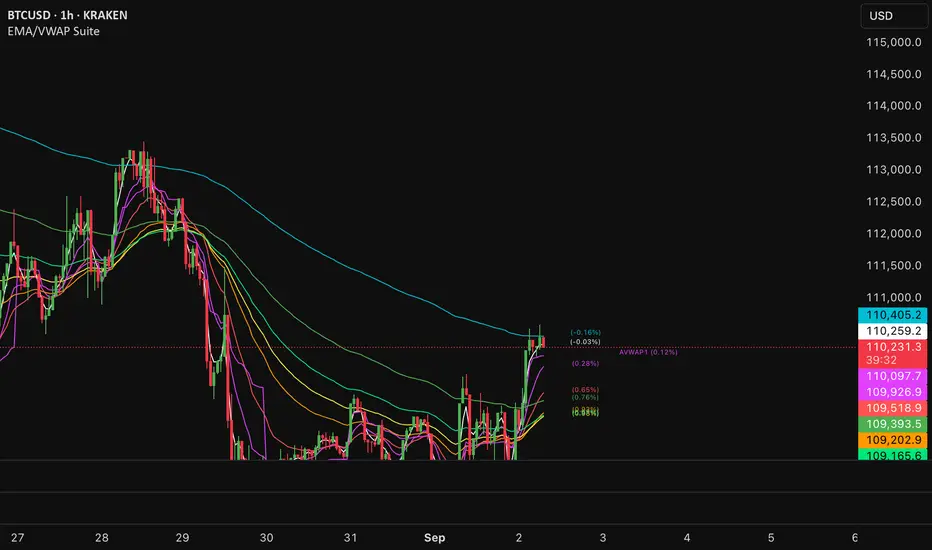
Primes_3These libraries (Primes_1 -> Primes_4) contain arrays of reduced Prime Numbers to minimize the amount of tokens, allowing more information to be exported.
Values, for example:
7001, 7013, 7019, 7027, 7039, 7043, 7057, 7069, 7079, 7103, 7109, 7021
are reduced to:
7001, 13, 19, 27, 39, 43, 57, 69, 79, 7103, 9, 21
With the restoreValues() function found in the Primes_4 library, the reduced values can be restored back to its original state.
7001, 13, 19, 27, 39, 43, 57, 69, 79, 7103, 9, 21
is restored back to:
7001, 7013, 7019, 7027, 7039, 7043, 7057, 7069, 7079, 7103, 7109, 7021
The libraries contain all Prime Numbers from 2 to 1.340.011
------------------------------------------------------------
Library "Primes_3"
Prime Numbers 713.021 - 1.095.989
primes_a()
Prime numbers 713.021 - 820.997
primes_b()
Prime numbers 821.003 - 928.979
primes_c()
Prime numbers 929.003 - 1.038.953
primes_d()
Prime numbers 1.039.001 - 1.095.989
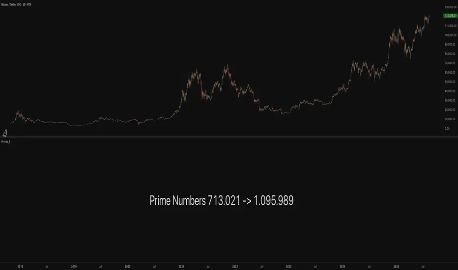
Primes_2These libraries (Primes_1 -> Primes_4) contain arrays of reduced Prime Numbers to minimize the amount of tokens, allowing more information to be exported.
Values, for example:
7001, 7013, 7019, 7027, 7039, 7043, 7057, 7069, 7079, 7103, 7109, 7021
are reduced to:
7001, 13, 19, 27, 39, 43, 57, 69, 79, 7103, 9, 21
With the restoreValues() function found in the Primes_4 library, the reduced values can be restored back to its original state.
7001, 13, 19, 27, 39, 43, 57, 69, 79, 7103, 9, 21
is restored back to:
7001, 7013, 7019, 7027, 7039, 7043, 7057, 7069, 7079, 7103, 7109, 7021
The libraries contain all Prime Numbers from 2 to 1.340.011
------------------------------------------------------------
Library "Primes_2"
Prime Numbers 340.007 - 712.981
primes_a()
Prime numbers 340.007 - 441.971
primes_b()
Prime numbers 442.003 - 545.959
primes_c()
Prime numbers 546.001 - 650.987
primes_d()
Prime numbers 651.017 - 712.981
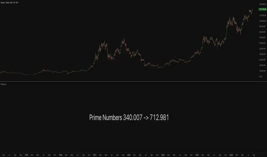
Primes_1These libraries (Primes_1 -> Primes_4) contain arrays of reduced Prime Numbers to minimize the amount of tokens, allowing more information to be exported.
Values, for example:
7001, 7013, 7019, 7027, 7039, 7043, 7057, 7069, 7079, 7103, 7109, 7021
are reduced to:
7001, 13, 19, 27, 39, 43, 57, 69, 79, 7103, 9, 21
With the restoreValues() function found in the Primes_4 library, the reduced values can be restored back to its original state.
7001, 13, 19, 27, 39, 43, 57, 69, 79, 7103, 9, 21
is restored back to:
7001, 7013, 7019, 7027, 7039, 7043, 7057, 7069, 7079, 7103, 7109, 7021
The libraries contain all Prime Numbers from 2 to 1.340.011
------------------------------------------------------------
Library "Primes_1"
Prime Numbers 2 - 339.991
primes_a()
Prime numbers 2 - 81.689
primes_b()
Prime numbers 81.701 - 175.897
primes_c()
Prime numbers 175.909 - 273.997
primes_d()
Prime numbers 274.007 - 339.991

Kelly Position Size CalculatorThis position sizing calculator implements the Kelly Criterion, developed by John L. Kelly Jr. at Bell Laboratories in 1956, to determine mathematically optimal position sizes for maximizing long-term wealth growth. Unlike arbitrary position sizing methods, this tool provides a scientifically solution based on your strategy's actual performance statistics and incorporates modern refinements from over six decades of academic research.
The Kelly Criterion addresses a fundamental question in capital allocation: "What fraction of capital should be allocated to each opportunity to maximize growth while avoiding ruin?" This question has profound implications for financial markets, where traders and investors constantly face decisions about optimal capital allocation (Van Tharp, 2007).
Theoretical Foundation
The Kelly Criterion for binary outcomes is expressed as f* = (bp - q) / b, where f* represents the optimal fraction of capital to allocate, b denotes the risk-reward ratio, p indicates the probability of success, and q represents the probability of loss (Kelly, 1956). This formula maximizes the expected logarithm of wealth, ensuring maximum long-term growth rate while avoiding the risk of ruin.
The mathematical elegance of Kelly's approach lies in its derivation from information theory. Kelly's original work was motivated by Claude Shannon's information theory (Shannon, 1948), recognizing that maximizing the logarithm of wealth is equivalent to maximizing the rate of information transmission. This connection between information theory and wealth accumulation provides a deep theoretical foundation for optimal position sizing.
The logarithmic utility function underlying the Kelly Criterion naturally embodies several desirable properties for capital management. It exhibits decreasing marginal utility, penalizes large losses more severely than it rewards equivalent gains, and focuses on geometric rather than arithmetic mean returns, which is appropriate for compounding scenarios (Thorp, 2006).
Scientific Implementation
This calculator extends beyond basic Kelly implementation by incorporating state of the art refinements from academic research:
Parameter Uncertainty Adjustment: Following Michaud (1989), the implementation applies Bayesian shrinkage to account for parameter estimation error inherent in small sample sizes. The adjustment formula f_adjusted = f_kelly × confidence_factor + f_conservative × (1 - confidence_factor) addresses the overconfidence bias documented by Baker and McHale (2012), where the confidence factor increases with sample size and the conservative estimate equals 0.25 (quarter Kelly).
Sample Size Confidence: The reliability of Kelly calculations depends critically on sample size. Research by Browne and Whitt (1996) provides theoretical guidance on minimum sample requirements, suggesting that at least 30 independent observations are necessary for meaningful parameter estimates, with 100 or more trades providing reliable estimates for most trading strategies.
Universal Asset Compatibility: The calculator employs intelligent asset detection using TradingView's built-in symbol information, automatically adapting calculations for different asset classes without manual configuration.
ASSET SPECIFIC IMPLEMENTATION
Equity Markets: For stocks and ETFs, position sizing follows the calculation Shares = floor(Kelly Fraction × Account Size / Share Price). This straightforward approach reflects whole share constraints while accommodating fractional share trading capabilities.
Foreign Exchange Markets: Forex markets require lot-based calculations following Lot Size = Kelly Fraction × Account Size / (100,000 × Base Currency Value). The calculator automatically handles major currency pairs with appropriate pip value calculations, following industry standards described by Archer (2010).
Futures Markets: Futures position sizing accounts for leverage and margin requirements through Contracts = floor(Kelly Fraction × Account Size / Margin Requirement). The calculator estimates margin requirements as a percentage of contract notional value, with specific adjustments for micro-futures contracts that have smaller sizes and reduced margin requirements (Kaufman, 2013).
Index and Commodity Markets: These markets combine characteristics of both equity and futures markets. The calculator automatically detects whether instruments are cash-settled or futures-based, applying appropriate sizing methodologies with correct point value calculations.
Risk Management Integration
The calculator integrates sophisticated risk assessment through two primary modes:
Stop Loss Integration: When fixed stop-loss levels are defined, risk calculation follows Risk per Trade = Position Size × Stop Loss Distance. This ensures that the Kelly fraction accounts for actual risk exposure rather than theoretical maximum loss, with stop-loss distance measured in appropriate units for each asset class.
Strategy Drawdown Assessment: For discretionary exit strategies, risk estimation uses maximum historical drawdown through Risk per Trade = Position Value × (Maximum Drawdown / 100). This approach assumes that individual trade losses will not exceed the strategy's historical maximum drawdown, providing a reasonable estimate for strategies with well-defined risk characteristics.
Fractional Kelly Approaches
Pure Kelly sizing can produce substantial volatility, leading many practitioners to adopt fractional Kelly approaches. MacLean, Sanegre, Zhao, and Ziemba (2004) analyze the trade-offs between growth rate and volatility, demonstrating that half-Kelly typically reduces volatility by approximately 75% while sacrificing only 25% of the growth rate.
The calculator provides three primary Kelly modes to accommodate different risk preferences and experience levels. Full Kelly maximizes growth rate while accepting higher volatility, making it suitable for experienced practitioners with strong risk tolerance and robust capital bases. Half Kelly offers a balanced approach popular among professional traders, providing optimal risk-return balance by reducing volatility significantly while maintaining substantial growth potential. Quarter Kelly implements a conservative approach with low volatility, recommended for risk-averse traders or those new to Kelly methodology who prefer gradual introduction to optimal position sizing principles.
Empirical Validation and Performance
Extensive academic research supports the theoretical advantages of Kelly sizing. Hakansson and Ziemba (1995) provide a comprehensive review of Kelly applications in finance, documenting superior long-term performance across various market conditions and asset classes. Estrada (2008) analyzes Kelly performance in international equity markets, finding that Kelly-based strategies consistently outperform fixed position sizing approaches over extended periods across 19 developed markets over a 30-year period.
Several prominent investment firms have successfully implemented Kelly-based position sizing. Pabrai (2007) documents the application of Kelly principles at Berkshire Hathaway, noting Warren Buffett's concentrated portfolio approach aligns closely with Kelly optimal sizing for high-conviction investments. Quantitative hedge funds, including Renaissance Technologies and AQR, have incorporated Kelly-based risk management into their systematic trading strategies.
Practical Implementation Guidelines
Successful Kelly implementation requires systematic application with attention to several critical factors:
Parameter Estimation: Accurate parameter estimation represents the greatest challenge in practical Kelly implementation. Brown (1976) notes that small errors in probability estimates can lead to significant deviations from optimal performance. The calculator addresses this through Bayesian adjustments and confidence measures.
Sample Size Requirements: Users should begin with conservative fractional Kelly approaches until achieving sufficient historical data. Strategies with fewer than 30 trades may produce unreliable Kelly estimates, regardless of adjustments. Full confidence typically requires 100 or more independent trade observations.
Market Regime Considerations: Parameters that accurately describe historical performance may not reflect future market conditions. Ziemba (2003) recommends regular parameter updates and conservative adjustments when market conditions change significantly.
Professional Features and Customization
The calculator provides comprehensive customization options for professional applications:
Multiple Color Schemes: Eight professional color themes (Gold, EdgeTools, Behavioral, Quant, Ocean, Fire, Matrix, Arctic) with dark and light theme compatibility ensure optimal visibility across different trading environments.
Flexible Display Options: Adjustable table size and position accommodate various chart layouts and user preferences, while maintaining analytical depth and clarity.
Comprehensive Results: The results table presents essential information including asset specifications, strategy statistics, Kelly calculations, sample confidence measures, position values, risk assessments, and final position sizes in appropriate units for each asset class.
Limitations and Considerations
Like any analytical tool, the Kelly Criterion has important limitations that users must understand:
Stationarity Assumption: The Kelly Criterion assumes that historical strategy statistics represent future performance characteristics. Non-stationary market conditions may invalidate this assumption, as noted by Lo and MacKinlay (1999).
Independence Requirement: Each trade should be independent to avoid correlation effects. Many trading strategies exhibit serial correlation in returns, which can affect optimal position sizing and may require adjustments for portfolio applications.
Parameter Sensitivity: Kelly calculations are sensitive to parameter accuracy. Regular calibration and conservative approaches are essential when parameter uncertainty is high.
Transaction Costs: The implementation incorporates user-defined transaction costs but assumes these remain constant across different position sizes and market conditions, following Ziemba (2003).
Advanced Applications and Extensions
Multi-Asset Portfolio Considerations: While this calculator optimizes individual position sizes, portfolio-level applications require additional considerations for correlation effects and aggregate risk management. Simplified portfolio approaches include treating positions independently with correlation adjustments.
Behavioral Factors: Behavioral finance research reveals systematic biases that can interfere with Kelly implementation. Kahneman and Tversky (1979) document loss aversion, overconfidence, and other cognitive biases that lead traders to deviate from optimal strategies. Successful implementation requires disciplined adherence to calculated recommendations.
Time-Varying Parameters: Advanced implementations may incorporate time-varying parameter models that adjust Kelly recommendations based on changing market conditions, though these require sophisticated econometric techniques and substantial computational resources.
Comprehensive Usage Instructions and Practical Examples
Implementation begins with loading the calculator on your desired trading instrument's chart. The system automatically detects asset type across stocks, forex, futures, and cryptocurrency markets while extracting current price information. Navigation to the indicator settings allows input of your specific strategy parameters.
Strategy statistics configuration requires careful attention to several key metrics. The win rate should be calculated from your backtest results using the formula of winning trades divided by total trades multiplied by 100. Average win represents the sum of all profitable trades divided by the number of winning trades, while average loss calculates the sum of all losing trades divided by the number of losing trades, entered as a positive number. The total historical trades parameter requires the complete number of trades in your backtest, with a minimum of 30 trades recommended for basic functionality and 100 or more trades optimal for statistical reliability. Account size should reflect your available trading capital, specifically the risk capital allocated for trading rather than total net worth.
Risk management configuration adapts to your specific trading approach. The stop loss setting should be enabled if you employ fixed stop-loss exits, with the stop loss distance specified in appropriate units depending on the asset class. For stocks, this distance is measured in dollars, for forex in pips, and for futures in ticks. When stop losses are not used, the maximum strategy drawdown percentage from your backtest provides the risk assessment baseline. Kelly mode selection offers three primary approaches: Full Kelly for aggressive growth with higher volatility suitable for experienced practitioners, Half Kelly for balanced risk-return optimization popular among professional traders, and Quarter Kelly for conservative approaches with reduced volatility.
Display customization ensures optimal integration with your trading environment. Eight professional color themes provide optimization for different chart backgrounds and personal preferences. Table position selection allows optimal placement within your chart layout, while table size adjustment ensures readability across different screen resolutions and viewing preferences.
Detailed Practical Examples
Example 1: SPY Swing Trading Strategy
Consider a professionally developed swing trading strategy for SPY (S&P 500 ETF) with backtesting results spanning 166 total trades. The strategy achieved 110 winning trades, representing a 66.3% win rate, with an average winning trade of $2,200 and average losing trade of $862. The maximum drawdown reached 31.4% during the testing period, and the available trading capital amounts to $25,000. This strategy employs discretionary exits without fixed stop losses.
Implementation requires loading the calculator on the SPY daily chart and configuring the parameters accordingly. The win rate input receives 66.3, while average win and loss inputs receive 2200 and 862 respectively. Total historical trades input requires 166, with account size set to 25000. The stop loss function remains disabled due to the discretionary exit approach, with maximum strategy drawdown set to 31.4%. Half Kelly mode provides the optimal balance between growth and risk management for this application.
The calculator generates several key outputs for this scenario. The risk-reward ratio calculates automatically to 2.55, while the Kelly fraction reaches approximately 53% before scientific adjustments. Sample confidence achieves 100% given the 166 trades providing high statistical confidence. The recommended position settles at approximately 27% after Half Kelly and Bayesian adjustment factors. Position value reaches approximately $6,750, translating to 16 shares at a $420 SPY price. Risk per trade amounts to approximately $2,110, representing 31.4% of position value, with expected value per trade reaching approximately $1,466. This recommendation represents the mathematically optimal balance between growth potential and risk management for this specific strategy profile.
Example 2: EURUSD Day Trading with Stop Losses
A high-frequency EURUSD day trading strategy demonstrates different parameter requirements compared to swing trading approaches. This strategy encompasses 89 total trades with a 58% win rate, generating an average winning trade of $180 and average losing trade of $95. The maximum drawdown reached 12% during testing, with available capital of $10,000. The strategy employs fixed stop losses at 25 pips and take profit targets at 45 pips, providing clear risk-reward parameters.
Implementation begins with loading the calculator on the EURUSD 1-hour chart for appropriate timeframe alignment. Parameter configuration includes win rate at 58, average win at 180, and average loss at 95. Total historical trades input receives 89, with account size set to 10000. The stop loss function is enabled with distance set to 25 pips, reflecting the fixed exit strategy. Quarter Kelly mode provides conservative positioning due to the smaller sample size compared to the previous example.
Results demonstrate the impact of smaller sample sizes on Kelly calculations. The risk-reward ratio calculates to 1.89, while the Kelly fraction reaches approximately 32% before adjustments. Sample confidence achieves 89%, providing moderate statistical confidence given the 89 trades. The recommended position settles at approximately 7% after Quarter Kelly application and Bayesian shrinkage adjustment for the smaller sample. Position value amounts to approximately $700, translating to 0.07 standard lots. Risk per trade reaches approximately $175, calculated as 25 pips multiplied by lot size and pip value, with expected value per trade at approximately $49. This conservative position sizing reflects the smaller sample size, with position sizes expected to increase as trade count surpasses 100 and statistical confidence improves.
Example 3: ES1! Futures Systematic Strategy
Systematic futures trading presents unique considerations for Kelly criterion application, as demonstrated by an E-mini S&P 500 futures strategy encompassing 234 total trades. This systematic approach achieved a 45% win rate with an average winning trade of $1,850 and average losing trade of $720. The maximum drawdown reached 18% during the testing period, with available capital of $50,000. The strategy employs 15-tick stop losses with contract specifications of $50 per tick, providing precise risk control mechanisms.
Implementation involves loading the calculator on the ES1! 15-minute chart to align with the systematic trading timeframe. Parameter configuration includes win rate at 45, average win at 1850, and average loss at 720. Total historical trades receives 234, providing robust statistical foundation, with account size set to 50000. The stop loss function is enabled with distance set to 15 ticks, reflecting the systematic exit methodology. Half Kelly mode balances growth potential with appropriate risk management for futures trading.
Results illustrate how favorable risk-reward ratios can support meaningful position sizing despite lower win rates. The risk-reward ratio calculates to 2.57, while the Kelly fraction reaches approximately 16%, lower than previous examples due to the sub-50% win rate. Sample confidence achieves 100% given the 234 trades providing high statistical confidence. The recommended position settles at approximately 8% after Half Kelly adjustment. Estimated margin per contract amounts to approximately $2,500, resulting in a single contract allocation. Position value reaches approximately $2,500, with risk per trade at $750, calculated as 15 ticks multiplied by $50 per tick. Expected value per trade amounts to approximately $508. Despite the lower win rate, the favorable risk-reward ratio supports meaningful position sizing, with single contract allocation reflecting appropriate leverage management for futures trading.
Example 4: MES1! Micro-Futures for Smaller Accounts
Micro-futures contracts provide enhanced accessibility for smaller trading accounts while maintaining identical strategy characteristics. Using the same systematic strategy statistics from the previous example but with available capital of $15,000 and micro-futures specifications of $5 per tick with reduced margin requirements, the implementation demonstrates improved position sizing granularity.
Kelly calculations remain identical to the full-sized contract example, maintaining the same risk-reward dynamics and statistical foundations. However, estimated margin per contract reduces to approximately $250 for micro-contracts, enabling allocation of 4-5 micro-contracts. Position value reaches approximately $1,200, while risk per trade calculates to $75, derived from 15 ticks multiplied by $5 per tick. This granularity advantage provides better position size precision for smaller accounts, enabling more accurate Kelly implementation without requiring large capital commitments.
Example 5: Bitcoin Swing Trading
Cryptocurrency markets present unique challenges requiring modified Kelly application approaches. A Bitcoin swing trading strategy on BTCUSD encompasses 67 total trades with a 71% win rate, generating average winning trades of $3,200 and average losing trades of $1,400. Maximum drawdown reached 28% during testing, with available capital of $30,000. The strategy employs technical analysis for exits without fixed stop losses, relying on price action and momentum indicators.
Implementation requires conservative approaches due to cryptocurrency volatility characteristics. Quarter Kelly mode is recommended despite the high win rate to account for crypto market unpredictability. Expected position sizing remains reduced due to the limited sample size of 67 trades, requiring additional caution until statistical confidence improves. Regular parameter updates are strongly recommended due to cryptocurrency market evolution and changing volatility patterns that can significantly impact strategy performance characteristics.
Advanced Usage Scenarios
Portfolio position sizing requires sophisticated consideration when running multiple strategies simultaneously. Each strategy should have its Kelly fraction calculated independently to maintain mathematical integrity. However, correlation adjustments become necessary when strategies exhibit related performance patterns. Moderately correlated strategies should receive individual position size reductions of 10-20% to account for overlapping risk exposure. Aggregate portfolio risk monitoring ensures total exposure remains within acceptable limits across all active strategies. Professional practitioners often consider using lower fractional Kelly approaches, such as Quarter Kelly, when running multiple strategies simultaneously to provide additional safety margins.
Parameter sensitivity analysis forms a critical component of professional Kelly implementation. Regular validation procedures should include monthly parameter updates using rolling 100-trade windows to capture evolving market conditions while maintaining statistical relevance. Sensitivity testing involves varying win rates by ±5% and average win/loss ratios by ±10% to assess recommendation stability under different parameter assumptions. Out-of-sample validation reserves 20% of historical data for parameter verification, ensuring that optimization doesn't create curve-fitted results. Regime change detection monitors actual performance against expected metrics, triggering parameter reassessment when significant deviations occur.
Risk management integration requires professional overlay considerations beyond pure Kelly calculations. Daily loss limits should cease trading when daily losses exceed twice the calculated risk per trade, preventing emotional decision-making during adverse periods. Maximum position limits should never exceed 25% of account value in any single position regardless of Kelly recommendations, maintaining diversification principles. Correlation monitoring reduces position sizes when holding multiple correlated positions that move together during market stress. Volatility adjustments consider reducing position sizes during periods of elevated VIX above 25 for equity strategies, adapting to changing market conditions.
Troubleshooting and Optimization
Professional implementation often encounters specific challenges requiring systematic troubleshooting approaches. Zero position size displays typically result from insufficient capital for minimum position sizes, negative expected values, or extremely conservative Kelly calculations. Solutions include increasing account size, verifying strategy statistics for accuracy, considering Quarter Kelly mode for conservative approaches, or reassessing overall strategy viability when fundamental issues exist.
Extremely high Kelly fractions exceeding 50% usually indicate underlying problems with parameter estimation. Common causes include unrealistic win rates, inflated risk-reward ratios, or curve-fitted backtest results that don't reflect genuine trading conditions. Solutions require verifying backtest methodology, including all transaction costs in calculations, testing strategies on out-of-sample data, and using conservative fractional Kelly approaches until parameter reliability improves.
Low sample confidence below 50% reflects insufficient historical trades for reliable parameter estimation. This situation demands gathering additional trading data, using Quarter Kelly approaches until reaching 100 or more trades, applying extra conservatism in position sizing, and considering paper trading to build statistical foundations without capital risk.
Inconsistent results across similar strategies often stem from parameter estimation differences, market regime changes, or strategy degradation over time. Professional solutions include standardizing backtest methodology across all strategies, updating parameters regularly to reflect current conditions, and monitoring live performance against expectations to identify deteriorating strategies.
Position sizes that appear inappropriately large or small require careful validation against traditional risk management principles. Professional standards recommend never risking more than 2-3% per trade regardless of Kelly calculations. Calibration should begin with Quarter Kelly approaches, gradually increasing as comfort and confidence develop. Most institutional traders utilize 25-50% of full Kelly recommendations to balance growth with prudent risk management.
Market condition adjustments require dynamic approaches to Kelly implementation. Trending markets may support full Kelly recommendations when directional momentum provides favorable conditions. Ranging or volatile markets typically warrant reducing to Half or Quarter Kelly to account for increased uncertainty. High correlation periods demand reducing individual position sizes when multiple positions move together, concentrating risk exposure. News and event periods often justify temporary position size reductions during high-impact releases that can create unpredictable market movements.
Performance monitoring requires systematic protocols to ensure Kelly implementation remains effective over time. Weekly reviews should compare actual versus expected win rates and average win/loss ratios to identify parameter drift or strategy degradation. Position size efficiency and execution quality monitoring ensures that calculated recommendations translate effectively into actual trading results. Tracking correlation between calculated and realized risk helps identify discrepancies between theoretical and practical risk exposure.
Monthly calibration provides more comprehensive parameter assessment using the most recent 100 trades to maintain statistical relevance while capturing current market conditions. Kelly mode appropriateness requires reassessment based on recent market volatility and performance characteristics, potentially shifting between Full, Half, and Quarter Kelly approaches as conditions change. Transaction cost evaluation ensures that commission structures, spreads, and slippage estimates remain accurate and current.
Quarterly strategic reviews encompass comprehensive strategy performance analysis comparing long-term results against expectations and identifying trends in effectiveness. Market regime assessment evaluates parameter stability across different market conditions, determining whether strategy characteristics remain consistent or require fundamental adjustments. Strategic modifications to position sizing methodology may become necessary as markets evolve or trading approaches mature, ensuring that Kelly implementation continues supporting optimal capital allocation objectives.
Professional Applications
This calculator serves diverse professional applications across the financial industry. Quantitative hedge funds utilize the implementation for systematic position sizing within algorithmic trading frameworks, where mathematical precision and consistent application prove essential for institutional capital management. Professional discretionary traders benefit from optimized position management that removes emotional bias while maintaining flexibility for market-specific adjustments. Portfolio managers employ the calculator for developing risk-adjusted allocation strategies that enhance returns while maintaining prudent risk controls across diverse asset classes and investment strategies.
Individual traders seeking mathematical optimization of capital allocation find the calculator provides institutional-grade methodology previously available only to professional money managers. The Kelly Criterion establishes theoretical foundation for optimal capital allocation across both single strategies and multiple trading systems, offering significant advantages over arbitrary position sizing methods that rely on intuition or fixed percentage approaches. Professional implementation ensures consistent application of mathematically sound principles while adapting to changing market conditions and strategy performance characteristics.
Conclusion
The Kelly Criterion represents one of the few mathematically optimal solutions to fundamental investment problems. When properly understood and carefully implemented, it provides significant competitive advantage in financial markets. This calculator implements modern refinements to Kelly's original formula while maintaining accessibility for practical trading applications.
Success with Kelly requires ongoing learning, systematic application, and continuous refinement based on market feedback and evolving research. Users who master Kelly principles and implement them systematically can expect superior risk-adjusted returns and more consistent capital growth over extended periods.
The extensive academic literature provides rich resources for deeper study, while practical experience builds the intuition necessary for effective implementation. Regular parameter updates, conservative approaches with limited data, and disciplined adherence to calculated recommendations are essential for optimal results.
References
Archer, M. D. (2010). Getting Started in Currency Trading: Winning in Today's Forex Market (3rd ed.). John Wiley & Sons.
Baker, R. D., & McHale, I. G. (2012). An empirical Bayes approach to optimising betting strategies. Journal of the Royal Statistical Society: Series D (The Statistician), 61(1), 75-92.
Breiman, L. (1961). Optimal gambling systems for favorable games. In J. Neyman (Ed.), Proceedings of the Fourth Berkeley Symposium on Mathematical Statistics and Probability (pp. 65-78). University of California Press.
Brown, D. B. (1976). Optimal portfolio growth: Logarithmic utility and the Kelly criterion. In W. T. Ziemba & R. G. Vickson (Eds.), Stochastic Optimization Models in Finance (pp. 1-23). Academic Press.
Browne, S., & Whitt, W. (1996). Portfolio choice and the Bayesian Kelly criterion. Advances in Applied Probability, 28(4), 1145-1176.
Estrada, J. (2008). Geometric mean maximization: An overlooked portfolio approach? The Journal of Investing, 17(4), 134-147.
Hakansson, N. H., & Ziemba, W. T. (1995). Capital growth theory. In R. A. Jarrow, V. Maksimovic, & W. T. Ziemba (Eds.), Handbooks in Operations Research and Management Science (Vol. 9, pp. 65-86). Elsevier.
Kahneman, D., & Tversky, A. (1979). Prospect theory: An analysis of decision under risk. Econometrica, 47(2), 263-291.
Kaufman, P. J. (2013). Trading Systems and Methods (5th ed.). John Wiley & Sons.
Kelly Jr, J. L. (1956). A new interpretation of information rate. Bell System Technical Journal, 35(4), 917-926.
Lo, A. W., & MacKinlay, A. C. (1999). A Non-Random Walk Down Wall Street. Princeton University Press.
MacLean, L. C., Sanegre, E. O., Zhao, Y., & Ziemba, W. T. (2004). Capital growth with security. Journal of Economic Dynamics and Control, 28(4), 937-954.
MacLean, L. C., Thorp, E. O., & Ziemba, W. T. (2011). The Kelly Capital Growth Investment Criterion: Theory and Practice. World Scientific.
Michaud, R. O. (1989). The Markowitz optimization enigma: Is 'optimized' optimal? Financial Analysts Journal, 45(1), 31-42.
Pabrai, M. (2007). The Dhandho Investor: The Low-Risk Value Method to High Returns. John Wiley & Sons.
Shannon, C. E. (1948). A mathematical theory of communication. Bell System Technical Journal, 27(3), 379-423.
Tharp, V. K. (2007). Trade Your Way to Financial Freedom (2nd ed.). McGraw-Hill.
Thorp, E. O. (2006). The Kelly criterion in blackjack sports betting, and the stock market. In L. C. MacLean, E. O. Thorp, & W. T. Ziemba (Eds.), The Kelly Capital Growth Investment Criterion: Theory and Practice (pp. 789-832). World Scientific.
Van Tharp, K. (2007). Trade Your Way to Financial Freedom (2nd ed.). McGraw-Hill Education.
Vince, R. (1992). The Mathematics of Money Management: Risk Analysis Techniques for Traders. John Wiley & Sons.
Vince, R., & Zhu, H. (2015). Optimal betting under parameter uncertainty. Journal of Statistical Planning and Inference, 161, 19-31.
Ziemba, W. T. (2003). The Stochastic Programming Approach to Asset, Liability, and Wealth Management. The Research Foundation of AIMR.
Further Reading
For comprehensive understanding of Kelly Criterion applications and advanced implementations:
MacLean, L. C., Thorp, E. O., & Ziemba, W. T. (2011). The Kelly Capital Growth Investment Criterion: Theory and Practice. World Scientific.
Vince, R. (1992). The Mathematics of Money Management: Risk Analysis Techniques for Traders. John Wiley & Sons.
Thorp, E. O. (2017). A Man for All Markets: From Las Vegas to Wall Street. Random House.
Cover, T. M., & Thomas, J. A. (2006). Elements of Information Theory (2nd ed.). John Wiley & Sons.
Ziemba, W. T., & Vickson, R. G. (Eds.). (2006). Stochastic Optimization Models in Finance. World Scientific.
