T3 ICL MACD STRATEGY
Backtested manually and received approx 60% winrate. Tradingview strategy tester is skewed because this program does not specify when to sell at profit target or at a stop loss.
Uses 1 min for entry and a longer time frame for confirmation (5,10,15, etc..) (Not sure what the yellow arrows are in the picture but they can be ignored)
Ideal Long Entry - The algo uses T3 moving average (T3) and the Ichimoku Conversion Line (ICL) to determine when to enter a long or short position. In this case we are going to showcase what causes the algo to alert long. It first checks to see if the the ICL is greater than T3. Once that condition is met T3 must be green in order to enter long and finally the last closing price has to be greater than the ICL. You can use the MACD to further verify a long trend as well!
Ideal Short Entry - The algo uses T3 moving average (T3) and the Ichimoku Conversion Line (ICL) to determine when to enter a long or short position. In this case we are going to showcase what causes the algo to alert short. It first checks to see if the the ICL is less than T3. Once that condition is met T3 must be red in order to enter short and finally the last closing price has to be less than the ICL. You can use the MACD to further verify a long trend as well!
在脚本中搜索"algo"

[PX] Moon PhaseHello guys,
while scrolling through the public library, I was surprised that there was no Open-Source version of the Moon Phase indicator. All moon phase indicators in the public library were either protected or not exactly what I was looking for. There is a built-in "Moon Phase" indicator, but even for this one, we can't access its source code.
Therefore, I started searching for an algorithm that I could implement into PineScript.
So here we go, an Open-Source Moon Phase indicator. It comes with the option to color the background based on the recent moon. Compared to the built-in indicator, the moon is slightly shifted, because it is centered on the candle and not plotted between two candles like the built-in indicator is doing it.
Feel free to use the indicator for your analysis or build on top of it in an open-source fashion.
Happy trading,
paaax :)
Reference: This indicator is a converted and simplified version of the original javascript algorithm, which can be found here .

SMU Quantum Thermo BallsThis script is the enhanced version of Market Thermometer with one difference. This one has Quantum Thermo balls shooting out of the thermometer tube when overheated. Quantum psychology, Quantum observation, call it what you like
My scripts are designed to beat ALGO, so the behavior of indicators is not like traditional indicators. Don't try to overthink it and compare it to other established functions.
If you knew ALGo as much as I do, then you would also ditch old indicators and design your own weird scripts to match the ALGO's personality. Oh yes, each AlGo for each stock has its own programming personality. Most my scripts are tuned to beat SPX ALGO meniac
Enjoy and think outside the box, the only way to beat the ALGO

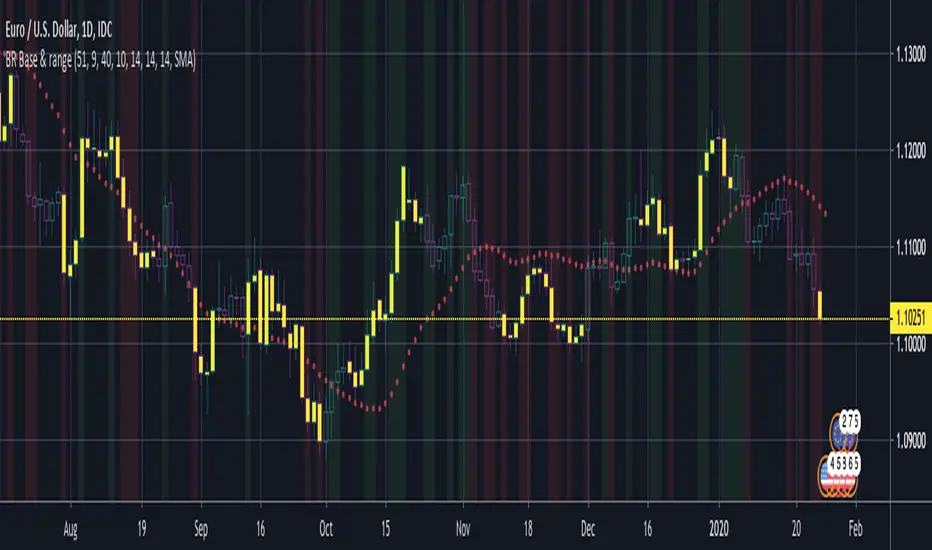
BERLIN Renegade - Baseline & RangeThis is the baseline and range candles part of a larger algorithm called the "BERLIN Renegade". It is based on the NNFX way of trading, with some modifications.
The baseline is used for price crossover signals, and consists of the LSMA. When price is below the baseline, the background turns red, and when it is above the baseline, the background turns green.
It also includes a modified version of the Range Identifier by LazyBear. This version calculates the same, but draws differently. It remove the baseline signal color if the Range Identifier signals there is a possible trading range forming.
The main way of identifying ranges is using the BERLIN Range Index. A panel version of this indicator is included in another part of the algorithm, but the bar color version is included here, to make the ranges even more visible and easier to avoid.
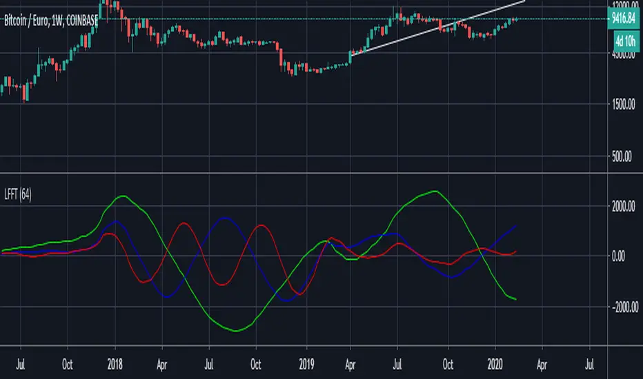
Low Frequency Fourier TransformThis Study uses the Real Discrete Fourier Transform algorithm to generate 3 sinusoids possibly indicative of future price.
I got information about this RDFT algorithm from "The Scientist and Engineer's Guide to Digital Signal Processing" By Steven W. Smith, Ph.D.
It has not been tested thoroughly yet, but it seems that that the RDFT isn't suited for predicting prices as the Frequency Domain Representation shows that the signal is similar to white noise, showing no significant peaks, indicative of very low periodicity of price movements.
Correlation MATRIX (Flexible version)Hey folks
A quick unrelated but interesting foreword
Hope you're all good and well and tanned
Me? I'm preparing the opening of my website where we're going to offer the Algorithm Builder Single Trend, Multiple Trends, Multi-Timeframe and plenty of others across many platforms (TradingView, FXCM, MT4, PRT). While others are at the beach and tanning (Yes I'm jealous, so what !?!), we're working our a** off to deliver an amazing looking website and great indicators and strategies for you guys.
Today I worked in including the Trade Manager Pro version and the Risk/Reward Pro version into all our Algorithm Builders. Here's a teaser
We're going to have a few indicators/strategies packages and subscriptions will open very soon.
The website should open in a few weeks and we still have loads to do ... (#no #summer #holidays #for #dave)
I see every message asking me to allow access to my Algorithm Builders but with the website opening shortly, it will be better for me to manage the trials from there - otherwise, it's duplicated and I can't follow all those requests
As you can probably all understand, it becomes very challenging to publish once a day with all that workload so I'll probably slow down (just a bit) and maybe posting once every 2/3 days until the website will be over (please forgive me for failing you). But once it will open, the daily publishing will resume again :) (here's when you're supposed to be clapping guys....)
While I'm so honored by all the likes, private messages and comments encouraging me, you have to realize that a script always takes me about 2/3 hours of work (with research, coding, debugging) but I'm doing it because I like it. Only pushing the brake a bit because of other constraints
INDICATOR OF THE DAY
I made a more flexible version of my Correlation Matrix .
You can now select the symbols you want and the matrix will update automatically !!! Let me repeat it once more because this is very cool... You can now select the symbols you want and the matrix will update automatically :)
Actually, I have nothing more to say about it... that's all :) Ah yes, I added a condition to detect negative correlation and they're being flagged with a black dot
Definition : Negative correlation or inverse correlation is a relationship between two variables whereby they move in opposite directions.
A negative correlation is a key concept in portfolio construction, as it enables the creation of diversified portfolios that can better withstand portfolio volatility and smooth out returns.
Correlation between two variables can vary widely over time. Stocks and bonds generally have a negative correlation, but in the decade to 2018, their correlation has ranged from -0.8 to 0.2. (Source : www.investopedia.com
See you maybe tomorrow or in a few days for another script/idea.
Be sure to hit the thumbs up to cheer me up as your likes will be the only sunlight I'll get for the next weeks.... because working on building a great offer for you guys.
Dave
____________________________________________________________
- I'm an officially approved PineEditor/LUA/MT4 approved mentor on codementor. You can request a coaching with me if you want and I'll teach you how to build kick-ass indicators and strategies
Jump on a 1 to 1 coaching with me
- You can also hire for a custom dev of your indicator/strategy/bot/chrome extension/python

SMA/pivot/Bollinger/MACD/RSI en pantalla gráficoMulti-indicador con los indicadores que empleo más pero sin añadir ventanas abajo.
Contiene:
Cruce de 3 medias móviles
La idea es no tenerlas en pantalla, pero están dibujadas también. Yo las dejo ocultas salvo que las quiera mirar para algo.
Lo que presento en pantalla es la media lenta con verde si el cruce de las 3 marca alcista, amarillo si no está claro y rojo si marca bajista.
Pivot
Normalmente los tengo ocultos pero los muestro cuando me interesa. Están todos aunque aparezcan 2 seguidos.
Bandas de Bollinger
No dibujo la línea central porque empleo la media como tal.
Parabollic SAR
Lo empleo para dibujar las ondas de Elliott como postula Matías Menéndez Larre en el capítulo 11 de su libro "Las ondas de Elliott". Así que, aunque se puede mostrar, lo mantengo oculto y lo que muestro es dónde cambia (SAR cambio).
MACD
No está dibujado porque necesitaría sacarlo del gráfico.
Marco en la parte superior cuándo la señal sobrepasa al MACD hacia arriba o hacia abajo con un flecha indicando el sentido de esta señal.
RSI
Similar al MACD pero en la parte inferior.
Probablemente, programe otro indicador para visualizar en una ventanita MACD, RSI y volumen todo junto. El volumen en la principal hay veces que no te permite ver bien alguna sombra y los otros 2 te quitan mucho espacio para graficar si los tienes permanentemente en 2 ventanas separadas.
DFT - Dominant Cycle Period 8-50 bars - John EhlerThis is the translation of discret cosine tranform (DCT) usage by John Ehler for finding dominant cycle period (DC).
The price is first filtered to remove aliasing noise(bellow 8 bars) and trend informations(above 50 bars), then the power is computed.
The trick here is to use a normalisation against the maximum power in order to get a good frequency resolution.
Current limitation in tradingview does not allow to display all of the periods, still the DC period is plot after beeing computed based on the center of gravity algo.
The DC period can be used to tune all of the indicators based on the cycles of the markets. For instance one can use this (DC period)/2 as an input for RSI.
Hope you find this of some interrest.
[naoligo] Simple ADXI'm publishing this indicator just for study purposes, because the result is exactly the same as DMI without the smoothing factor. It is exactly the same as ADX Wilder from MT5.
I was looking for the algorithm all over and it was a pain to find the right formula, meaning: one that would match with the built-in ones. After several study and comparison, I still didn't find the algorithm that match with the MT5's built-in simple ADX ...
Enjoy!

Patrones de entrada/salida V.1.0 -BETA-Este algoritmo intenta identificar patrones o fractales dentro de los movimientos de precios para dar señales de compra o venta de activos.

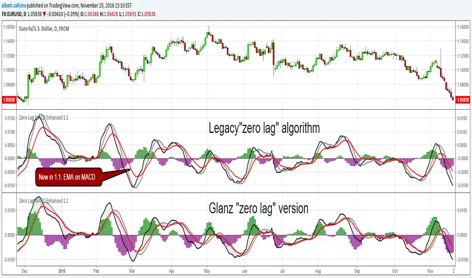
Zero Lag MACD Enhanced - Version 1.1ENHANCED ZERO LAG MACD
Version 1.1
Based on ZeroLag EMA - see Technical Analysis of Stocks and Commodities, April 2000
Original version by user Glaz. Thanks !
Ideas and code from @yassotreyo version.
Tweaked by Albert Callisto (AC)
New features:
Added original signal line formula
Added optional EMA on MACD
Added filling between the MACD and signal line
I looked at other versions of the zero lag and noticed that the histogram was slightly different. After looking at other zero lags on TV, I noticed that the algorithm implementation of Glanz generated a modified signal line. I decided to add the old version to be compliant with the original algorithm that you will find in other platforms like MT4, FXCM, etc.
So now you can choose if you want the original algorithm or Glanz version. It's up to you then to choose which one you prefer. I also added an extra EMA applied on the MACD. This is used in a system I am currently studying and can be of some interest to filter out false signals.
Acc/Dist. Cloud with Fractal Deviation Bands by @XeL_ArjonaACCUMULATION / DISTRIBUTION CLOUD with MORPHIC DEVIATION BANDS
Ver. 2.0.beta.23:08:2015
by Ricardo M. Arjona @XeL_Arjona
DISCLAIMER
The Following indicator/code IS NOT intended to be a formal investment advice or recommendation by the author, nor should be construed as such. Users will be fully responsible by their use regarding their own trading vehicles/assets.
The embedded code and ideas within this work are FREELY AND PUBLICLY available on the Web for NON LUCRATIVE ACTIVITIES and must remain as is.
Pine Script code MOD's and adaptations by @XeL_Arjona with special mention in regard of:
Buy (Bull) and Sell (Bear) "Power Balance Algorithm by Vadim Gimelfarb published at Stocks & Commodities V. 21:10 (68-72).
Custom Weighting Coefficient for Exponential Moving Average (nEMA) adaptation work by @XeL_Arjona with contribution help from @RicardoSantos at TradingView @pinescript chat room.
Morphic Numbers (PHI & Plastic) Pine Script adaptation from it's algebraic generation formulas by @XeL_Arjona
Fractal Deviation Bands idea by @XeL_Arjona
CHANGE LOG:
ACCUMULATION / DISTRIBUTION CLOUD: I decided to change it's name from the Buy to Sell Pressure. The code is essentially the same as older versions and they are the center core (VORTEX?) of all derived New stuff which are:
MORPHIC NUMBERS: The "Golden Ratio" expressed by the result of the constant "PHI" and the newer and same in characteristics "Plastic Number" expressed as "PN". For more information about this regard take a look at: HERE!
CUSTOM(K) EXPONENTIAL MOVING AVERAGE: Some code has cleaned from last version to include as custom function the nEMA , which use an additional input (K) to customise the way the "exponentially" is weighted from the custom array. For the purpose of this indicator, I implement a volatility algorithm using the Average True Range of last 9 periods multiplied by the morphic number used in the fractal study. (Golden Ratio as default) The result is very similar in response to classic EMA but tend to accelerate or decelerate much more responsive with wider bars presented in trending average.
FRACTAL DEVIATION BANDS: The main idea is based on the so useful Standard Deviation process to create Bands in favor of a multiplier (As John Bollinger used in it's own bands) from a custom array, in which for this case is the "Volume Pressure Moving Average" as the main Vortex for the "Fractallitly", so then apply as many "Child bands" using the older one as the new calculation array using the same morphic constant as multiplier (Like Fibonacci but with other approach rather than %ratios). Results are AWSOME! Market tend to accelerate or decelerate their Trend in favor of a Fractal approach. This bands try to catch them, so please experiment and feedback me your own observations.
EXTERNAL TICKER FOR VOLUME DATA: I Added a way to input volume data for this kind of study from external tickers. This is just a quicky-hack given that currently TradingView is not adding Volume to their Indexes so; maybe this is temporary by now. It seems that this part of the code is conflicting with intraday timeframes, so You are advised.
This CODE is versioned as BETA FOR TESTING PROPOSES. By now TradingView Admins are changing lot's of things internally, so maybe this could conflict with correct rendering of this study with special tickers or timeframes. I will try to code by itself just the core parts of this study in order to use them at discretion in other areas. ALL NEW IDEAS OR MODIFICATIONS to these indicator(s) are Welcome in favor to deploy a better and more accurate readings. I will be very glad to be notified at Twitter or TradingView accounts at: @XeL_Arjona

ChunkbrAI-NN INDIChunkbrAI-NN INDI: The Neural Network Odyssey
A Native Pine Script Neural Network Research Engine
Welcome to ChunkbrAI-NN 5.3. This is not a standard technical indicator; it is a proof-of-concept Artificial Intelligence engine built entirely from scratch within Pine Script.
Neural Networks typically require iterating over massive datasets, a task that usually times out on TradingView. ChunkbrAI solves this by introducing a novel "Chunking Architecture"—a system that breaks history into digestible learning blocks and trains a Multilayer Perceptron (MLP) using a "Chunking" approach.
It features a living ecosystem where neurons have "genes," grow mature, and adapt to market regimes using a highly sophisticated Context-Aware normalization engine.
-----------------------------------------------------------
The Core Concept: "The Time Wheel"
To bypass Pine Script's execution limits, this script does not train linearly from the beginning of time. Instead, it operates like a spinning wheel of experience.
* The Chunk System: On every bar update, the engine reaches back into history (up to 5000 bars) and grabs random or sequential "Chunks" of data. It treats these chunks as isolated training samples.
* Experience Replay: By constantly revisiting past market scenarios (Chunks), the network slowly converges its weights, learning to recognize patterns across different eras of price action.
-----------------------------------------------------------
Architecture & Modules
A. The Neural Core (MLP)
At the heart is a raw neural network built with arrays:
* Topology: A dense network with a customizable Hidden Layer (Default: 60 Neurons).
* Timewarp (Stride): When enabled, the network uses "dilated" inputs (skipping bars, e.g., 1, 3, 5...). This increases the network's Field of View without increasing computational load.
* Forecasting: The network outputs a standardized prediction which is then de-normalized to project the future price path on your chart.
B. The Context System (The "Eyes")
Raw prices confuse neural networks. A $1000 move in Bitcoin is massive in 2016 but noise in 2024. ChunkbrAI uses a relativistic Context System:
* Regime Detection: It uses a Zero-Lag Moving Average (ZLMA) and Non-Linear Regression to measure the current market "Vibe" (Volatility & Trend).
* Dynamic Normalization: The inputs are scaled based on this context. If the market is volatile, the data is compressed; if calm, it is expanded. This ensures the brain receives consistent signal patterns regardless of the absolute price.
C. The Gene System (Neuro-Plasticity)
This is the experimental "biology" layer. Neurons are not just static math; they have life cycles.
* Maturity: Neurons start "Young" (highly plastic, high mutation rate). As they successfully reduce error, they become "Wise" (stable, low mutation).
* Mutation: If a "Wise" neuron begins failing (high error), it is demoted and forced to mutate. This allows the brain to "forget" obsolete behaviors and adapt to new market paradigms automatically.
* Profiles: You can initialize the brain with different personalities (e.g., Dreamer, Young Chaos, Zen Monk).
D. The Brain Scheduler (Adaptive Learning)
A static Learning Rate (LR) is inefficient. The Brain Scheduler acts as the heartbeat:
* Panic vs. Flow: It monitors the derivative of the error. If the error spikes (Panic), the Scheduler slows down learning to prevent the model from exploding. If the error smooths out (Flow), it accelerates learning (Infinite LR Mode).
-----------------------------------------------------------
Forecasting Modes
The script provides two distinct ways to visualize the future:
1. Direct Projection (Green Line):
The network takes the current window of price action and predicts the immediate next step. If Timewarp is active, it interpolates the result to draw a smooth curve.
2. Autoregression (Cyan Line):
Available in "Auto" mode. The network feeds its *own* predictions back into itself as inputs to generate multi-step forecasts.
* Wave Segmentation: The script intelligently guesses the current market cycle length and attempts to project that specific duration forward.
-----------------------------------------------------------
Operation Manual
The script has two distinct training loops: first, when you add it to a chart, Pine runs through the available historical bars once, and this initial history pass is the main training phase where the network iterates chunk-by-chunk using your configured chunk count/iterations (e.g., if chunk count is 3, it performs 3 chunk updates per step), but pushing chunk count, iterations, or model sizing too high can hit Pine’s execution limits; after that, once real-time candles start printing, the script can either keep training (weights continue updating) or freeze the weights and run inference only, producing predictions from the learned parameters, and if live training is enabled it can also simulate “bars-back” style training during live mode by iterating across prior bars as if doing another history pass—which again can run into limits if chunks/iterations/sizing are too heavy—so when changing parameters to evaluate behavior you change them carefully and individually, because multiple simultaneous increases make it hard to attribute effects and can more easily trigger those execution constraints.
Weight Persistence (Save/Load):
Pine Script can’t write files or persist weights directly, so ChunkbrAI uses a library-based workaround that’s honestly tricky and kind of a pain: you enable the weight-export alerts so the script emits the weights (W1/W2/biases etc.) as text, and those payloads are chunked as well; then, outside TradingView, I use a separate Python script to parse the alert emails, reconstruct and format the chunked weights properly, and generate the corresponding library code files; after that, the libraries have to be published/updated, and only then can the main script “restore” by reading the published lib constants on chart load, effectively starting with the pre-trained weights instead of relying purely on the fresh history-run training pass. I don’t recommend this process unless you really have to—it’s fragile and high-effort—but until TradingView implements some simple built-in data storage for scripts, it’s basically the only practical way to save and reload your models.
-----------------------------------------------------------
Limitations & Notes
* Calculation Limits: This script pushes Pine Script to its absolute edge. If you increase Chunk Size or Hidden Size too much, you WILL hit execution limits. Use the defaults as a baseline.
* Non-Deterministic: Because the "Wheel" picks random chunks for training, two instances of this script might evolve slightly different brains unless you use the Restore Weights feature.
* Experimental: This is a research tool designed to explore Neural Networks and Genetic Algorithms on the chart. Treat it as an educational engine, not financial advice.
Credits: Concept and Engineering by funkybrown.

Break & Retest 369Break & Retest 369
The Break & Retest 369 is a high-precision technical indicator designed for price action traders who specialize in market structure shifts and "S/R Flip" (Support becoming Resistance and vice versa) strategies. Unlike standard oscillators that lag behind price, this tool focuses on **horizontal price levels** that have historically acted as turning points, providing visual zones where the market is likely to offer a "second chance" entry.
Core Philosophy
The script is built on the principle of Market Memory. In a trending market, a "Breakout" signifies a change in order flow. However, smart money often returns to the point of origin (the breakout level) to fill remaining orders or test the strength of the new trend. This indicator automates the identification of these "Retest" zones, which are often the highest-probability entry points for trend continuation.
How It Works: The Logic
The indicator follows a strict, multi-step calculation process:
1. Swing Point Identification: It utilizes a Pivot High/Low** algorithm. It scans for "peaks" and "valleys" that are isolated by a specific number of bars on either side (defined by the `Lookback` input).
2. **Breakout Detection:** The script monitors these pivot levels. A **Buy Zone** is triggered only when the price achieves a clean **Close** above a previous Pivot High. Conversely, a **Sell Zone** is triggered by a **Close** below a previous Pivot Low.
3. **Zone Construction:** Once a break is confirmed, the script draws a box centered exactly at the price level of the broken pivot.
4. **Forward Projection:** These zones are projected forward in time using the `Zone Extension` parameter, creating a visual "landing strip" for future price action.
### Key Features & How to Use It
* **Dynamic Support/Resistance Flips:** Green zones represent former resistance levels that are now expected to act as support. Red zones represent former support levels now expected to act as resistance.
* **Zone Customization:** Traders can adjust the `Zone Height (Ticks)` to account for market volatility or specific asset spreads (e.g., wider zones for XAUUSD, tighter for EURUSD).
* **Scannability:** The script helps traders filter out the "noise" of mid-range price movement and focus only on significant structural levels.
### Default Configuration
To get the most out of the **369** logic, the indicator comes pre-configured with the following defaults:
* **Swing Detection Lookback (18):** Optimized for medium-term structure, avoiding "micro-pivots" that lead to false signals.
* **Zone Height (1 Tick):** Focuses on the precise price point of the pivot for maximum accuracy.
* **Zone Extension (90 Bars):** Projects levels far enough to catch "deep" retests that occur several hours or days later.
---
### Pro Tip for Traders
Wait for price to return to a **Buy Zone** and look for a bullish rejection candle (like a pin bar or engulfing candle) before entering. This combines the "Where" (the zone) with the "When" (the price action confirmation) for a robust trading system.
Would you like me to add a **"Mitigation"** feature that automatically deletes or fades the zone once the price has successfully touched it?

Neeson RSI Divergence DetectorIntegrating Multi-Indicator Strategies: A Rational Approach to Technical Analysis Tools
Introduction
The integration of multiple technical indicators into a unified trading script represents a sophisticated approach to market analysis, combining complementary analytical methods to enhance decision-making. This article outlines the rational basis for combining specific indicators, explains their synergistic operation, and provides practical guidance for users seeking to understand the functional utility, operational mechanics, and unique value proposition of integrated technical analysis tools.
Functional Purpose and Rational Integration Basis
Integrated technical scripts are designed to address the inherent limitations of single-indicator analysis by combining multiple analytical perspectives. The rational basis for integration typically follows these principles:
Complementary Signal Validation: Different indicators measure distinct market characteristics (momentum, volatility, trend strength, etc.). Their combination allows cross-validation of signals, reducing false positives inherent in single-indicator systems.
Multi-Timeframe Confirmation: Integrated scripts often incorporate elements that analyze price action across different temporal dimensions, providing a more comprehensive market perspective.
Risk Management Enhancement: By combining overbought/oversold indicators with trend confirmation tools, these scripts help identify not only entry opportunities but also potential risk zones.
Market Phase Adaptation: Different market conditions (trending, ranging, volatile) favor different indicator types. Integrated approaches maintain relevance across varying market environments.
Synergistic Operational Mechanism
The components of well-designed integrated scripts operate through several synergistic mechanisms:
Primary Trend Identification: Core trend-following indicators establish the dominant market direction, serving as a filter for other signals. This prevents counter-trend entries that might otherwise be generated by oscillators or momentum indicators.
Momentum Confirmation: Oscillator-based components (like RSI or Stochastic) validate the strength of the identified trend, distinguishing between healthy retracements and potential reversals.
Divergence Detection: By comparing price action with momentum indicators, these scripts identify subtle shifts in market dynamics that often precede trend changes.
Volatility Adjustment: Volatility-based components dynamically adjust signal thresholds and position sizing recommendations based on current market conditions.
Multi-Layer Filtering: Each signal passes through successive validation layers, with only the strongest, most confirmed signals triggering alerts or visual markers.
Practical Application Guidance
Users can maximize the utility of integrated scripts through these practical approaches:
Parameter Customization: Adjust indicator periods and thresholds to match the characteristics of specific trading instruments and timeframes. Historical testing can identify optimal settings for particular markets.
Signal Hierarchy Interpretation: Learn to distinguish between primary signals (strongly confirmed across multiple indicators) and secondary signals (weaker confirmation) for appropriate position sizing.
Contextual Analysis: Consider integrated signals within the broader market context, including support/resistance levels, volume patterns, and fundamental developments.
Performance Correlation: Monitor how different market conditions affect script performance. Some configurations may excel in trending markets while others perform better in ranging conditions.
Risk Calibration: Use the multi-indicator confirmation to calibrate stop-loss and take-profit levels, with tighter parameters for strongly confirmed signals and wider parameters for weaker ones.
Originality and Value Proposition
The originality of well-designed integrated scripts manifests in several dimensions:
Unique Combination Logic: The specific selection and weighting of indicators, along with their integration methodology, represents intellectual value distinct from simple indicator stacking.
Innovative Signal Processing: Advanced scripts often incorporate proprietary algorithms for signal filtering, noise reduction, or probability weighting not found in standard indicators.
Adaptive Framework: Some scripts dynamically adjust their analytical approach based on changing market conditions, representing a form of artificial market intelligence.
Visualization Innovation: The presentation of complex multi-indicator data in an intuitive, actionable format constitutes significant user interface originality.
Empirical Limitations and Responsible Use
It is crucial to maintain realistic expectations regarding integrated technical scripts:
No Predictive Certainty: These tools analyze probabilities, not certainties. No combination of historical price indicators can guarantee future price movements.
Market Efficiency Limitations: All technical analysis operates within the constraints of market efficiency, with script effectiveness varying across different market conditions and time periods.
Complementary Role: Integrated scripts should complement, not replace, comprehensive trading strategies including risk management, fundamental analysis, and market knowledge.
Continuous Evaluation: Regular performance assessment against established benchmarks helps maintain realistic expectations and identifies when script adjustments may be necessary.
Conclusion
The thoughtful integration of multiple technical indicators represents a logical evolution in analytical methodology, addressing the limitations of single-indicator approaches through complementary validation and multi-dimensional analysis. By understanding the rational basis for integration, the synergistic operation of components, and the practical application parameters, users can employ these tools as valuable components within broader, disciplined trading approaches. The true value emerges not from predictive accuracy but from structured decision support that helps traders navigate complex market environments with greater consistency and insight.

Gold Intelligence - Final Sniper v12 by Herman Sangivera(Papua)🚀 Gold Intelligence - Final Sniper v12 by Herman Sangivera ( Papua )
Overview
Gold Intelligence - Final Sniper v12 is a cutting-edge technical indicator specifically engineered for high-volatility instruments like XAU/USD (Gold). This indicator merges advanced Price Action candlestick recognition algorithms with institutional volume analysis and real-time market sentiment to deliver precision entry signals.
The primary goal of this tool is to filter out market "noise" and highlight only High Probability Setups that meet strict technical criteria.
🛡️ Key Features
Smart Pattern Recognition: Automatically identifies high-impact patterns: Pin Bars (psychological rejection) and Engulfing Candles (institutional dominance).
Probability Scoring: Every signal is assigned a percentage (%) score based on volume confirmation and price intensity. Signals only trigger when they exceed the minimum threshold (default 75%).
Real-Time Sentiment Dashboard: An exclusive on-chart panel that monitors the balance of Buy/Sell pressure instantly.
Dynamic Risk Management: Automatically projects Take Profit (TP) and Stop Loss (SL) boxes using Average True Range (ATR) calculations, ensuring your targets stay adaptive to current market volatility.
Institutional Volume Check: Validates entries by cross-referencing significant volume spikes (Smart Money footprints) to help you avoid market traps and fakeouts.
📖 How to Use (Trading Guide)
Identify the Signal: Wait for the "SNAPSHOT GOLD" label to appear on the chart.
🟢 Green Label: Buy Signal (Bullish).
🔴 Red Label: Sell Signal (Bearish).
Check Probability Score: It is highly recommended to only take signals with a score of >75%. A higher score indicates stronger technical confluence.
Execution & Targets:
Enter the trade at the close of the signal candle.
Target the Green transparent box for profit and use the Red box for risk management.
Dashboard Confirmation: Ensure the Sentiment percentage aligns with your trade direction (e.g., Sentiment > 60% Buy for Long positions).
⚙️ Input Parameters
Min Probability: The minimum accuracy threshold for a signal to be displayed.
TP & SL Multiplier: Customize your reward-to-risk ratio based on ATR multiples.
Alerts: Fully compatible with real-time notifications for Mobile, Email, or Webhooks.
⚠️ Disclaimer
This indicator is an analytical tool and does not guarantee profits. Gold trading involves significant risk. Always use proper money management and backtest on a demo account before trading live funds.
