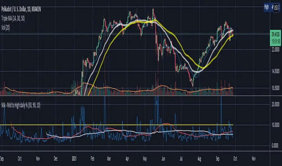
MACD Forecast Colorful [DiFlip]MACD Forecast Colorful
The Future of Predictive MACD — is one of the most advanced and customizable MACD indicators ever published on TradingView. Built on the classic MACD foundation, this upgraded version integrates statistical forecasting through linear regression to anticipate future movements — not just react to the past.
With a total of 22 fully configurable long and short entry conditions, visual enhancements, and full automation support, this indicator is designed for serious traders seeking an analytical edge.
⯁ Real-Time MACD Forecasting
For the first time, a public MACD script combines the classic structure of MACD with predictive analytics powered by linear regression. Instead of simply responding to current values, this tool projects the MACD line, signal line, and histogram n bars into the future, allowing you to trade with foresight rather than hindsight.
⯁ Fully Customizable
This indicator is built for flexibility. It includes 22 entry conditions, all of which are fully configurable. Each condition can be turned on/off, chained using AND/OR logic, and adapted to your trading model.
Whether you're building a rules-based quant system, automating alerts, or refining discretionary signals, MACD Forecast Colorful gives you full control over how signals are generated, displayed, and triggered.
⯁ With MACD Forecast Colorful, you can:
• Detect MACD crossovers before they happen.
• Anticipate trend reversals with greater precision.
• React earlier than traditional indicators.
• Gain a powerful edge in both discretionary and automated strategies.
• This isn’t just smarter MACD — it’s predictive momentum intelligence.
⯁ Scientifically Powered by Linear Regression
MACD Forecast Colorful is the first public MACD indicator to apply least-squares predictive modeling to MACD behavior — effectively introducing machine learning logic into a time-tested tool.
It uses statistical regression to analyze historical behavior of the MACD and project future trajectories. The result is a forward-shifted MACD forecast that can detect upcoming crossovers and divergences before they appear on the chart.
⯁ Linear Regression: Technical Foundation
Linear regression is a statistical method that models the relationship between a dependent variable (y) and one or more independent variables (x). The basic formula for simple linear regression is:
y = β₀ + β₁x + ε
Where:
y = predicted variable (e.g., future MACD value)
x = independent variable (e.g., bar index)
β₀ = intercept
β₁ = slope
ε = random error (residual)
The regression model calculates β₀ and β₁ using the least squares method, minimizing the sum of squared prediction errors to produce the best-fit line through historical values. This line is then extended forward, generating a forecast based on recent price momentum.
⯁ Least Squares Estimation
The regression coefficients are computed with the following formulas:
β₁ = Σ((xᵢ - x̄)(yᵢ - ȳ)) / Σ((xᵢ - x̄)²)
β₀ = ȳ - β₁x̄
Where:
Σ denotes summation; x̄ and ȳ are the means of x and y; and i ranges from 1 to n (number of observations). These equations produce the best linear unbiased estimator under the Gauss–Markov assumptions — constant variance (homoscedasticity) and a linear relationship between variables.
⯁ Regression in Machine Learning
Linear regression is a foundational model in supervised learning. Its ability to provide precise, explainable, and fast forecasts makes it critical in AI systems and quantitative analysis.
Applying linear regression to MACD forecasting is the equivalent of injecting artificial intelligence into one of the most widely used momentum tools in trading.
⯁ Visual Interpretation
Picture the MACD values over time like this:
Time →
MACD →
A regression line is fitted to recent MACD values, then projected forward n periods. The result is a predictive trajectory that can cross over the real MACD or signal line — offering an early-warning system for trend shifts and momentum changes.
The indicator plots both current MACD and forecasted MACD, allowing you to visually compare short-term future behavior against historical movement.
⯁ Scientific Concepts Used
Linear Regression: models the relationship between variables using a straight line.
Least Squares Method: minimizes squared prediction errors for best-fit.
Time-Series Forecasting: projects future data based on past patterns.
Supervised Learning: predictive modeling using labeled inputs.
Statistical Smoothing: filters noise to highlight trends.
⯁ Why This Indicator Is Revolutionary
First open-source MACD with real-time predictive modeling.
Scientifically grounded with linear regression logic.
Automatable through TradingView alerts and bots.
Smart signal generation using forecasted crossovers.
Highly customizable with 22 buy/sell conditions.
Enhanced visuals with background (bgcolor) and area fill (fill) support.
This isn’t just an update — it’s the next evolution of MACD forecasting.
⯁ Example of simple linear regression with one independent variable
This example demonstrates how a basic linear regression works when there is only one independent variable influencing the dependent variable. This type of model is used to identify a direct relationship between two variables.
⯁ In linear regression, observations (red) are considered the result of random deviations (green) from an underlying relationship (blue) between a dependent variable (y) and an independent variable (x)
This concept illustrates that sampled data points rarely align perfectly with the true trend line. Instead, each observed point represents the combination of the true underlying relationship and a random error component.
⯁ Visualizing heteroscedasticity in a scatterplot with 100 random fitted values using Matlab
Heteroscedasticity occurs when the variance of the errors is not constant across the range of fitted values. This visualization highlights how the spread of data can change unpredictably, which is an important factor in evaluating the validity of regression models.
⯁ The datasets in Anscombe’s quartet were designed to have nearly the same linear regression line (as well as nearly identical means, standard deviations, and correlations) but look very different when plotted
This classic example shows that summary statistics alone can be misleading. Even with identical numerical metrics, the datasets display completely different patterns, emphasizing the importance of visual inspection when interpreting a model.
⯁ Result of fitting a set of data points with a quadratic function
This example illustrates how a second-degree polynomial model can better fit certain datasets that do not follow a linear trend. The resulting curve reflects the true shape of the data more accurately than a straight line.
⯁ What is the MACD?
The Moving Average Convergence Divergence (MACD) is a technical analysis indicator developed by Gerald Appel. It measures the relationship between two moving averages of a security’s price to identify changes in momentum, direction, and strength of a trend. The MACD is composed of three components: the MACD line, the signal line, and the histogram.
⯁ How to use the MACD?
The MACD is calculated by subtracting the 26-period Exponential Moving Average (EMA) from the 12-period EMA. A 9-period EMA of the MACD line, called the signal line, is then plotted on top of the MACD line. The MACD histogram represents the difference between the MACD line and the signal line.
Here are the primary signals generated by the MACD:
• Bullish Crossover: When the MACD line crosses above the signal line, indicating a potential buy signal.
• Bearish Crossover: When the MACD line crosses below the signal line, indicating a potential sell signal.
• Divergence: When the price of the security diverges from the MACD, suggesting a potential reversal.
• Overbought/Oversold Conditions: Indicated by the MACD line moving far away from the signal line, though this is less common than in oscillators like the RSI.
⯁ How to use MACD forecast?
The MACD Forecast is built on the same foundation as the classic MACD, but with predictive capabilities.
Step 1 — Spot Predicted Crossovers:
Watch for forecasted bullish or bearish crossovers. These signals anticipate when the MACD line will cross the signal line in the future, letting you prepare trades before the move.
Step 2 — Confirm with Histogram Projection:
Use the projected histogram to validate momentum direction. A rising histogram signals strengthening bullish momentum, while a falling projection points to weakening or bearish conditions.
Step 3 — Combine with Multi-Timeframe Analysis:
Use forecasts across multiple timeframes to confirm signal strength (e.g., a 1h forecast aligned with a 4h forecast).
Step 4 — Set Entry Conditions & Automation:
Customize your buy/sell rules with the 20 forecast-based conditions and enable automation for bots or alerts.
Step 5 — Trade Ahead of the Market:
By preparing for future momentum shifts instead of reacting to the past, you’ll always stay one step ahead of lagging traders.
📈 BUY
🍟 Signal Validity: The signal will remain valid for X bars.
🍟 Signal Sequence: Configurable as AND or OR.
🍟 MACD > Signal Smoothing
🍟 MACD < Signal Smoothing
🍟 Histogram > 0
🍟 Histogram < 0
🍟 Histogram Positive
🍟 Histogram Negative
🍟 MACD > 0
🍟 MACD < 0
🍟 Signal > 0
🍟 Signal < 0
🍟 MACD > Histogram
🍟 MACD < Histogram
🍟 Signal > Histogram
🍟 Signal < Histogram
🍟 MACD (Crossover) Signal
🍟 MACD (Crossunder) Signal
🍟 MACD (Crossover) 0
🍟 MACD (Crossunder) 0
🍟 Signal (Crossover) 0
🍟 Signal (Crossunder) 0
🔮 MACD (Crossover) Signal Forecast
🔮 MACD (Crossunder) Signal Forecast
📉 SELL
🍟 Signal Validity: The signal will remain valid for X bars.
🍟 Signal Sequence: Configurable as AND or OR.
🍟 MACD > Signal Smoothing
🍟 MACD < Signal Smoothing
🍟 Histogram > 0
🍟 Histogram < 0
🍟 Histogram Positive
🍟 Histogram Negative
🍟 MACD > 0
🍟 MACD < 0
🍟 Signal > 0
🍟 Signal < 0
🍟 MACD > Histogram
🍟 MACD < Histogram
🍟 Signal > Histogram
🍟 Signal < Histogram
🍟 MACD (Crossover) Signal
🍟 MACD (Crossunder) Signal
🍟 MACD (Crossover) 0
🍟 MACD (Crossunder) 0
🍟 Signal (Crossover) 0
🍟 Signal (Crossunder) 0
🔮 MACD (Crossover) Signal Forecast
🔮 MACD (Crossunder) Signal Forecast
🤖 Automation
All BUY and SELL conditions can be automated using TradingView alerts. Every configurable condition can trigger alerts suitable for fully automated or semi-automated strategies.
⯁ Unique Features
Linear Regression: (Forecast)
Signal Validity: The signal will remain valid for X bars
Signal Sequence: Configurable as AND/OR
Table of Conditions: BUY/SELL
Conditions Label: BUY/SELL
Plot Labels in the graph above: BUY/SELL
Automate & Monitor Signals/Alerts: BUY/SELL
Background Colors: "bgcolor"
Background Colors: "fill"
Linear Regression (Forecast)
Signal Validity: The signal will remain valid for X bars
Signal Sequence: Configurable as AND/OR
Table of Conditions: BUY/SELL
Conditions Label: BUY/SELL
Plot Labels in the graph above: BUY/SELL
Automate & Monitor Signals/Alerts: BUY/SELL
Background Colors: "bgcolor"
Background Colors: "fill"
在脚本中搜索"bot"
AliceTears GridAliceTears Grid is a customizable Mean Reversion system designed to capitalize on market volatility during specific trading sessions. Unlike standard grid bots that place blind limit orders, this strategy establishes a daily or session-based "Baseline" and looks for price over-extensions to fade the move back to the mean.
This strategy is best suited for ranging markets (sideways accumulation) or specific forex sessions (e.g., Asian Session or NY/London overlap) where price tends to revert to the opening price.
🛠 How It Works
1. The Baseline & Grid Generation At the start of every session (or the daily open), the script records the Open price. It then projects visual grid lines above and below this price based on your Step % input.
Example: If the Open is $100 and Step is 1%, lines are drawn at $101, $102, $99, $98, etc.
2. Entry Logic: Reversal Mode This script features a "Reversal Mode" (enabled by default) to filter out "falling knives."
Standard Grid: Buys immediately when price touches the line.
AliceTears Logic: Waits for the price to breach a grid level and then close back inside towards the mean. This confirms a potential rejection of that level before entering.
3. Exit Logic
Target Profit: The primary target is the previous grid level (Mean Reversion).
Trailing Stop: If the price continues moving in your favor, a trailing stop activates to maximize the run.
Stop Loss: A manual percentage-based stop loss is available to prevent deep drawdowns in trending markets.
⚙️ Key Features
Visual Grid: Automatically draws entry levels on the chart for the current session, helping you visualize where the "math" is waiting for price.
Timezone & Session Control: Includes a custom Timezone Offset tool. You can trade specific hours (e.g., 09:30–16:00) regardless of your chart's UTC setting.
Grid Management: Independent logic for Long and Short grids with pyramiding capabilities.
Safety Filters: Options to force-close trades at the end of the session to avoid overnight gaps.
⚠️ Risk Warning
Please Read Before Using: This is a Counter-Trend / Grid Strategy.
Pros: High win rate in sideways/ranging markets.
Cons: In strong trending markets (parabolic pumps or crashes), this strategy will add to losing positions ("catch a falling knife").
Recommendation: Always use the Stop Loss and Date Filter inputs. Do not run this on highly volatile assets without strict risk management parameters.
Settings Guide
Entry Reversal Mode: Keep checked for safer entries. Uncheck for aggressive limit-order style execution.
Grid Step (%): The distance between lines. For Forex, use lower values (0.1% - 0.5%). For Crypto, use higher values (1.0% - 3.0%).
UTC Offset: Adjust this to align the Session Hours with your target market (e.g., -5 for New York).
This script is open source. Feel free to use it for educational purposes or modify it to fit your trading style.
AB=CD Fibonacci Strategy (One Trade at a Time)
AB=CD Fibonacci Strategy - Harmonic Pattern Trading Bot
Description
An automated trading strategy that identifies and trades the classic AB=CD harmonic pattern, one of the most reliable geometric price formations in technical analysis. This strategy detects perfectly proportioned Fibonacci retracement setups and executes trades with precise risk-reward management.
How It Works
The indicator scans for the AB=CD pattern structure:
Leg AB: Initial swing from pivot point A to pivot point B
Leg BC: Retracement to point C (customizable Fibonacci levels)
Leg CD: Mirror projection equal to the AB leg length
When price touches point D, the strategy automatically enters a position with predefined take-profit and stop-loss levels based on your risk-reward ratio.
Key Features
One Trade at a Time: Ensures disciplined position management by allowing only one active trade per pattern
Customizable Fibonacci Retracement: Set your preferred retracement range for point C (default 50% - 78.6%)
Risk-Reward Control: Adjust stop-loss and take-profit multiples to match your trading plan
Visual Pattern Display: Clear labeling of A, B, C, D points with pattern lines for easy identification
Both Directions: Identifies bullish and bearish AB=CD patterns automatically
Ideal For
Swing traders on higher timeframes (4H, Daily, Weekly)
Harmonic pattern traders seeking automation
Traders wanting precise entry and exit rules based on Fibonacci geometry
Those looking to reduce emotional trading and increase consistency
Default Settings Optimized For
NASDAQ futures and currency pairs
Medium timeframe analysis
Conservative risk management (10% position size per trade)
Fibot X: GALA Auto StrategyFibot X — GALA Optimized is an algorithmic trading system designed specifically for the GALA/USDT asset.
The algorithm manages trades automatically through a structured multi-target exit model and a predefined stop-loss risk control.
It operates fully autonomously — no external indicators, no manual decisions.
This version is the result of extensive analysis of real market conditions for GALA and comes fully configured.
Users are not required to modify any parameters: the system is pre-calibrated to provide optimal performance while minimizing complexity.
⚠️ Critical Operational Requirements
🔹 Timeframe: 30 minutes only.
All trend detection, entry logic and management layers were engineered and validated exclusively on the 30m timeframe.
Using any other timeframe breaks the model.
🔹 Leverage: strictly x1.
Higher leverage disrupts the internal balance of the strategy and significantly increases risk exposure beyond its intended design.
🔹 Capital Use: 100% allocation.
The take-profit architecture and drawdown control are designed around full equity usage — not partial positions, scaling, or incremental sizing.
Consistency Through System Design
Fibot X does not chase micro-fluctuations, noise or aggressive scalping.
Its purpose is to capture meaningful market swings and convert them into structured profits through intelligent partial exits, avoiding overexposure and premature re-entries.
For long-term stability, the most effective approach is to use multiple Fibot X bots across different assets simultaneously.
Diversifying execution distributes volatility, smooths equity curves and increases system consistency over time — without requiring user intervention.
Philosophy
The strategy’s internal parameters are continuously updated based on performance metrics, ensuring alignment with evolving market conditions and maximizing efficiency within a controlled risk framework.
Fibot X requires no external indicators and no constant monitoring.
Its design is simple: automation, discipline, and consistent execution.
Super-AO with Risk Management Alerts Template - 11-29-25Super-AO with Risk Management: ALERTS & AUTOMATION Edition
Signal Lynx | Free Scripts supporting Automation for the Night-Shift Nation 🌙
1. Overview
This is the Indicator / Alerts companion to the Super-AO Strategy.
While the Strategy version is built for backtesting (verifying profitability and checking historical performance), this Indicator version is built for Live Execution.
We understand the frustration of finding a great strategy, only to realize you can't easily hook it up to your trading bot. This script solves that. It contains the exact same "Super-AO" logic and "Risk Management Engine" as the strategy version, but it is optimized to send signals to automation platforms like Signal Lynx, 3Commas, or any Webhook listener.
2. Quick Action Guide (TL;DR)
Purpose: Live Signal Generation & Automation.
Workflow:
Use the Strategy Version to find profitable settings.
Copy those settings into this Indicator Version.
Set a TradingView Alert using the "Any Alert() function call" condition.
Best Timeframe: 4 Hours (H4) and above.
Compatibility: Works with any webhook-based automation service.
3. Why Two Scripts?
Pine Script operates in two distinct modes:
Strategy Mode: Calculates equity, drawdowns, and simulates orders. Great for research, but sometimes complex to automate.
Indicator Mode: Plots visual data on the chart. This is the preferred method for setting up robust alerts because it is lighter weight and plots specific values that automation services can read easily.
The Golden Rule: Always backtest on the Strategy, but trade on the Indicator. This ensures that what you see in your history matches what you execute in real-time.
4. How to Automate This Script
This script uses a "Visual Spike" method to trigger alerts. Instead of drawing equity curves, it plots numerical values at the bottom of your chart when a trade event occurs.
The Signal Map:
Blue Spike (2 / -2): Entry Signal (Long / Short).
Yellow Spike (1 / -1): Risk Management Close (Stop Loss / Trend Reversal).
Green Spikes (1, 2, 3): Take Profit Levels 1, 2, and 3.
Setup Instructions:
Add this indicator to your chart.
Open your TradingView "Alerts" tab.
Create a new Alert.
Condition: Select SAO - RM Alerts Template.
Trigger: Select Any Alert() function call.
Message: Paste your JSON webhook message (provided by your bot service).
5. The Logic Under the Hood
Just like the Strategy version, this indicator utilizes:
SuperTrend + Awesome Oscillator: High-probability swing trading logic.
Non-Repainting Engine: Calculates signals based on confirmed candle closes to ensure the alert you get matches the chart reality.
Advanced Adaptive Trailing Stop (AATS): Internally calculates volatility to determine when to send a "Close" signal.
6. About Signal Lynx
Automation for the Night-Shift Nation 🌙
We are providing this code open source to help traders bridge the gap between manual backtesting and live automation. This code has been in action since 2022.
If you are looking to automate your strategies, please take a look at Signal Lynx in your search.
License: Mozilla Public License 2.0 (Open Source). If you make beneficial modifications, please release them back to the community!
G-BOT ENGULFING CANDLE - FIXED SL & TP // Description:
This Pine Script strategy identifies bullish and bearish engulfing candle patterns over a defined lookback period and places trades based
on recent market highs and lows. It calculates stop loss and take profit levels using the Average True Range (ATR) multiplied by a user-defined factor, with the ability to adjust the risk-to-reward ratio for each trade.
Zonas de Liquidez Pro + Puntos de GiroRequirements for marking 💧:✅ High crosses the zone✅ Close returns inside (false breakout / fakeout)✅ Volume is 20% greater than the average✅ Occurs within the last 10 bars(Note: This last requirement is stated in the text but not explicitly in the code snippet provided)📚 Psychology Behind the SweepWho lost money?Traders with stops placed too tightlyBuyers who entered "on the breakout"Bots with automatic orders placed aboveWho made money?Smart Money / InstitutionsThey sold at a high priceThey hunted for liquidity before moving the priceThey know where retail stops are located🎯 How to Use the Drops in Your TradingGolden Rule:💧 near a strong zone + Multiple rejections = PROBABLE REVERSALStrategy:See 💧 at resistance → Look for SHORTSee 💧 at support → Look for LONGPrice returns to the swept zone → High-probability setupStop beyond the sweep high/low → ProtectionPractical Example:If you see 💧 LIQ at $111,263 (resistance)→ Wait for bearish rejection→ Entry: Sell at $110,800→ Stop: $111,500 (above the sweep high)→ Target: Next support level⚠️ Common Mistakes❌ Mistake 1: Trading the breakoutPrice breaks $111k → "It's going to the moon!" → Buy💧 LIQ appears → It was a trap → Drop → Loss✅ Correct Approach:Price breaks $111k → Check if there is 💧 LIQ💧 appears → "It's a trap" → Wait for rejection → Sell❌ Mistake 2: Ignoring the volumeNot all sweeps are equal.Sweeps with high volume are more reliable.No volume = it could be noise.🎓 Ultra-Fast SummaryElementMeaning💧 LIQLiquidity sweep detectedAt ResistanceBullish trap → Prepare for a shortAt SupportBearish trap → Prepare for a longWith High VolumeMore reliable signalNear Strong Zone High probability of reversal🔥 The Magic of Your IndicatorScenarioWithout this IndicatorWith this IndicatorAction"The price broke $111k, I'm buying!""There is 💧 LIQ + zone + rejections → It's a trap."ResultYou loseYou avoid a loss or gain on the short
DarkPool's Gann High Low Activator DarkPool's Gann High-Low Activator.
It enhances the traditional trend-following logic by integrating Heikin Ashi smoothing, Multi-Timeframe (MTF) analysis, and volatility filtering. It is designed to filter out market noise and provide clearer trend signals during volatile conditions.
Underlying Concepts
Heikin Ashi Smoothing: Standard price candles can produce erratic signals due to wicks and short-term volatility. This script includes a "Calculation Mode" setting that allows the Gann logic to run on Heikin Ashi average prices. This smoothes out price data, helping traders stay in trends longer by ignoring temporary pullbacks.
Gann High-Low Logic: The core algorithm tracks the Simple Moving Average (SMA) of Highs and Lows over a user-defined period.
Bullish Trend: Price closes above the trailing SMA of Highs.
Bearish Trend: Price closes below the trailing SMA of Lows.
Volatility & Trend Filtering: To reduce false signals during sideways markets, this tool employs two filters:
ADX Filter (Choppiness): Uses the Average Directional Index to detect low-volatility environments. If the ADX is below the defined threshold (default 20), the indicator identifies the market as "choppy" and suppresses signals to preserve capital.
EMA Filter (Baseline): An optional Exponential Moving Average filter ensures trades are only taken in the direction of the longer-term trend (e.g., Longs only above the 200 EMA).
Features
Dual Calculation Modes: Switch between Standard price logic and Heikin Ashi smoothing logic.
Multi-Timeframe (MTF): Calculate the trend based on a higher timeframe (e.g., 4-Hour) while viewing a lower timeframe chart (e.g., 15-Minute).
Automated JSON Alerts: Generates machine-readable JSON alert payloads compatible with external trading bots and webhooks.
Live Dashboard: A data table displaying the current Trend State, Calculation Mode, ADX Value, and risk percentage.
How to Use
Buy Signal: Generated when the trend flips Bullish, provided the ADX indicates sufficient momentum and the price satisfies the EMA filter (if enabled).
Sell Signal: Generated when the trend flips Bearish, subject to the same momentum and trend filters.
Neutral State (Gray Cloud): When the cloud fill turns gray, the market is in consolidation. It is recommended to avoid entering new positions during this state.
Trailing Stop: The Gann Line serves as a dynamic trailing stop-loss level. A close beyond this line invalidates the current trend.
Settings Configuration
Calculation Mode: Select "Standard" for raw price action or "Heikin Ashi" for smoothed trend following.
Gann Length: Lower values (3-5) are suitable for short-term scalping; higher values (10+) are better for swing trading.
MTF Mode: Enable to lock the calculation to a specific higher timeframe.
ADX Threshold: Adjust based on asset volatility. Recommended: 20-25 for Crypto, 15-20 for Forex/Indices.
Disclaimer
This source code and the information presented here are for educational purposes only. This script does not constitute financial advice, trading recommendations, or a solicitation to buy or sell any financial instruments. Trading in financial markets involves a high degree of risk and may not be suitable for all investors. Past performance is not indicative of future results. The author assumes no responsibility for any losses incurred while using this indicator. Use this tool at your own discretion and risk.
Dimensional Resonance ProtocolDimensional Resonance Protocol
🌀 CORE INNOVATION: PHASE SPACE RECONSTRUCTION & EMERGENCE DETECTION
The Dimensional Resonance Protocol represents a paradigm shift from traditional technical analysis to complexity science. Rather than measuring price levels or indicator crossovers, DRP reconstructs the hidden attractor governing market dynamics using Takens' embedding theorem, then detects emergence —the rare moments when multiple dimensions of market behavior spontaneously synchronize into coherent, predictable states.
The Complexity Hypothesis:
Markets are not simple oscillators or random walks—they are complex adaptive systems existing in high-dimensional phase space. Traditional indicators see only shadows (one-dimensional projections) of this higher-dimensional reality. DRP reconstructs the full phase space using time-delay embedding, revealing the true structure of market dynamics.
Takens' Embedding Theorem (1981):
A profound mathematical result from dynamical systems theory: Given a time series from a complex system, we can reconstruct its full phase space by creating delayed copies of the observation.
Mathematical Foundation:
From single observable x(t), create embedding vectors:
X(t) =
Where:
• d = Embedding dimension (default 5)
• τ = Time delay (default 3 bars)
• x(t) = Price or return at time t
Key Insight: If d ≥ 2D+1 (where D is the true attractor dimension), this embedding is topologically equivalent to the actual system dynamics. We've reconstructed the hidden attractor from a single price series.
Why This Matters:
Markets appear random in one dimension (price chart). But in reconstructed phase space, structure emerges—attractors, limit cycles, strange attractors. When we identify these structures, we can detect:
• Stable regions : Predictable behavior (trade opportunities)
• Chaotic regions : Unpredictable behavior (avoid trading)
• Critical transitions : Phase changes between regimes
Phase Space Magnitude Calculation:
phase_magnitude = sqrt(Σ ² for i = 0 to d-1)
This measures the "energy" or "momentum" of the market trajectory through phase space. High magnitude = strong directional move. Low magnitude = consolidation.
📊 RECURRENCE QUANTIFICATION ANALYSIS (RQA)
Once phase space is reconstructed, we analyze its recurrence structure —when does the system return near previous states?
Recurrence Plot Foundation:
A recurrence occurs when two phase space points are closer than threshold ε:
R(i,j) = 1 if ||X(i) - X(j)|| < ε, else 0
This creates a binary matrix showing when the system revisits similar states.
Key RQA Metrics:
1. Recurrence Rate (RR):
RR = (Number of recurrent points) / (Total possible pairs)
• RR near 0: System never repeats (highly stochastic)
• RR = 0.1-0.3: Moderate recurrence (tradeable patterns)
• RR > 0.5: System stuck in attractor (ranging market)
• RR near 1: System frozen (no dynamics)
Interpretation: Moderate recurrence is optimal —patterns exist but market isn't stuck.
2. Determinism (DET):
Measures what fraction of recurrences form diagonal structures in the recurrence plot. Diagonals indicate deterministic evolution (trajectory follows predictable paths).
DET = (Recurrence points on diagonals) / (Total recurrence points)
• DET < 0.3: Random dynamics
• DET = 0.3-0.7: Moderate determinism (patterns with noise)
• DET > 0.7: Strong determinism (technical patterns reliable)
Trading Implication: Signals are prioritized when DET > 0.3 (deterministic state) and RR is moderate (not stuck).
Threshold Selection (ε):
Default ε = 0.10 × std_dev means two states are "recurrent" if within 10% of a standard deviation. This is tight enough to require genuine similarity but loose enough to find patterns.
🔬 PERMUTATION ENTROPY: COMPLEXITY MEASUREMENT
Permutation entropy measures the complexity of a time series by analyzing the distribution of ordinal patterns.
Algorithm (Bandt & Pompe, 2002):
1. Take overlapping windows of length n (default n=4)
2. For each window, record the rank order pattern
Example: → pattern (ranks from lowest to highest)
3. Count frequency of each possible pattern
4. Calculate Shannon entropy of pattern distribution
Mathematical Formula:
H_perm = -Σ p(π) · ln(p(π))
Where π ranges over all n! possible permutations, p(π) is the probability of pattern π.
Normalized to :
H_norm = H_perm / ln(n!)
Interpretation:
• H < 0.3 : Very ordered, crystalline structure (strong trending)
• H = 0.3-0.5 : Ordered regime (tradeable with patterns)
• H = 0.5-0.7 : Moderate complexity (mixed conditions)
• H = 0.7-0.85 : Complex dynamics (challenging to trade)
• H > 0.85 : Maximum entropy (nearly random, avoid)
Entropy Regime Classification:
DRP classifies markets into five entropy regimes:
• CRYSTALLINE (H < 0.3): Maximum order, persistent trends
• ORDERED (H < 0.5): Clear patterns, momentum strategies work
• MODERATE (H < 0.7): Mixed dynamics, adaptive required
• COMPLEX (H < 0.85): High entropy, mean reversion better
• CHAOTIC (H ≥ 0.85): Near-random, minimize trading
Why Permutation Entropy?
Unlike traditional entropy methods requiring binning continuous data (losing information), permutation entropy:
• Works directly on time series
• Robust to monotonic transformations
• Computationally efficient
• Captures temporal structure, not just distribution
• Immune to outliers (uses ranks, not values)
⚡ LYAPUNOV EXPONENT: CHAOS vs STABILITY
The Lyapunov exponent λ measures sensitivity to initial conditions —the hallmark of chaos.
Physical Meaning:
Two trajectories starting infinitely close will diverge at exponential rate e^(λt):
Distance(t) ≈ Distance(0) × e^(λt)
Interpretation:
• λ > 0 : Positive Lyapunov exponent = CHAOS
- Small errors grow exponentially
- Long-term prediction impossible
- System is sensitive, unpredictable
- AVOID TRADING
• λ ≈ 0 : Near-zero = CRITICAL STATE
- Edge of chaos
- Transition zone between order and disorder
- Moderate predictability
- PROCEED WITH CAUTION
• λ < 0 : Negative Lyapunov exponent = STABLE
- Small errors decay
- Trajectories converge
- System is predictable
- OPTIMAL FOR TRADING
Estimation Method:
DRP estimates λ by tracking how quickly nearby states diverge over a rolling window (default 20 bars):
For each bar i in window:
δ₀ = |x - x | (initial separation)
δ₁ = |x - x | (previous separation)
if δ₁ > 0:
ratio = δ₀ / δ₁
log_ratios += ln(ratio)
λ ≈ average(log_ratios)
Stability Classification:
• STABLE : λ < 0 (negative growth rate)
• CRITICAL : |λ| < 0.1 (near neutral)
• CHAOTIC : λ > 0.2 (strong positive growth)
Signal Filtering:
By default, NEXUS requires λ < 0 (stable regime) for signal confirmation. This filters out trades during chaotic periods when technical patterns break down.
📐 HIGUCHI FRACTAL DIMENSION
Fractal dimension measures self-similarity and complexity of the price trajectory.
Theoretical Background:
A curve's fractal dimension D ranges from 1 (smooth line) to 2 (space-filling curve):
• D ≈ 1.0 : Smooth, persistent trending
• D ≈ 1.5 : Random walk (Brownian motion)
• D ≈ 2.0 : Highly irregular, space-filling
Higuchi Method (1988):
For a time series of length N, construct k different curves by taking every k-th point:
L(k) = (1/k) × Σ|x - x | × (N-1)/(⌊(N-m)/k⌋ × k)
For different values of k (1 to k_max), calculate L(k). The fractal dimension is the slope of log(L(k)) vs log(1/k):
D = slope of log(L) vs log(1/k)
Market Interpretation:
• D < 1.35 : Strong trending, persistent (Hurst > 0.5)
- TRENDING regime
- Momentum strategies favored
- Breakouts likely to continue
• D = 1.35-1.45 : Moderate persistence
- PERSISTENT regime
- Trend-following with caution
- Patterns have meaning
• D = 1.45-1.55 : Random walk territory
- RANDOM regime
- Efficiency hypothesis holds
- Technical analysis least reliable
• D = 1.55-1.65 : Anti-persistent (mean-reverting)
- ANTI-PERSISTENT regime
- Oscillator strategies work
- Overbought/oversold meaningful
• D > 1.65 : Highly complex, choppy
- COMPLEX regime
- Avoid directional bets
- Wait for regime change
Signal Filtering:
Resonance signals (secondary signal type) require D < 1.5, indicating trending or persistent dynamics where momentum has meaning.
🔗 TRANSFER ENTROPY: CAUSAL INFORMATION FLOW
Transfer entropy measures directed causal influence between time series—not just correlation, but actual information transfer.
Schreiber's Definition (2000):
Transfer entropy from X to Y measures how much knowing X's past reduces uncertainty about Y's future:
TE(X→Y) = H(Y_future | Y_past) - H(Y_future | Y_past, X_past)
Where H is Shannon entropy.
Key Properties:
1. Directional : TE(X→Y) ≠ TE(Y→X) in general
2. Non-linear : Detects complex causal relationships
3. Model-free : No assumptions about functional form
4. Lag-independent : Captures delayed causal effects
Three Causal Flows Measured:
1. Volume → Price (TE_V→P):
Measures how much volume patterns predict price changes.
• TE > 0 : Volume provides predictive information about price
- Institutional participation driving moves
- Volume confirms direction
- High reliability
• TE ≈ 0 : No causal flow (weak volume/price relationship)
- Volume uninformative
- Caution on signals
• TE < 0 (rare): Suggests price leading volume
- Potentially manipulated or thin market
2. Volatility → Momentum (TE_σ→M):
Does volatility expansion predict momentum changes?
• Positive TE : Volatility precedes momentum shifts
- Breakout dynamics
- Regime transitions
3. Structure → Price (TE_S→P):
Do support/resistance patterns causally influence price?
• Positive TE : Structural levels have causal impact
- Technical levels matter
- Market respects structure
Net Causal Flow:
Net_Flow = TE_V→P + 0.5·TE_σ→M + TE_S→P
• Net > +0.1 : Bullish causal structure
• Net < -0.1 : Bearish causal structure
• |Net| < 0.1 : Neutral/unclear causation
Causal Gate:
For signal confirmation, NEXUS requires:
• Buy signals : TE_V→P > 0 AND Net_Flow > 0.05
• Sell signals : TE_V→P > 0 AND Net_Flow < -0.05
This ensures volume is actually driving price (causal support exists), not just correlated noise.
Implementation Note:
Computing true transfer entropy requires discretizing continuous data into bins (default 6 bins) and estimating joint probability distributions. NEXUS uses a hybrid approach combining TE theory with autocorrelation structure and lagged cross-correlation to approximate information transfer in computationally efficient manner.
🌊 HILBERT PHASE COHERENCE
Phase coherence measures synchronization across market dimensions using Hilbert transform analysis.
Hilbert Transform Theory:
For a signal x(t), the Hilbert transform H (t) creates an analytic signal:
z(t) = x(t) + i·H (t) = A(t)·e^(iφ(t))
Where:
• A(t) = Instantaneous amplitude
• φ(t) = Instantaneous phase
Instantaneous Phase:
φ(t) = arctan(H (t) / x(t))
The phase represents where the signal is in its natural cycle—analogous to position on a unit circle.
Four Dimensions Analyzed:
1. Momentum Phase : Phase of price rate-of-change
2. Volume Phase : Phase of volume intensity
3. Volatility Phase : Phase of ATR cycles
4. Structure Phase : Phase of position within range
Phase Locking Value (PLV):
For two signals with phases φ₁(t) and φ₂(t), PLV measures phase synchronization:
PLV = |⟨e^(i(φ₁(t) - φ₂(t)))⟩|
Where ⟨·⟩ is time average over window.
Interpretation:
• PLV = 0 : Completely random phase relationship (no synchronization)
• PLV = 0.5 : Moderate phase locking
• PLV = 1 : Perfect synchronization (phases locked)
Pairwise PLV Calculations:
• PLV_momentum-volume : Are momentum and volume cycles synchronized?
• PLV_momentum-structure : Are momentum cycles aligned with structure?
• PLV_volume-structure : Are volume and structural patterns in phase?
Overall Phase Coherence:
Coherence = (PLV_mom-vol + PLV_mom-struct + PLV_vol-struct) / 3
Signal Confirmation:
Emergence signals require coherence ≥ threshold (default 0.70):
• Below 0.70: Dimensions not synchronized, no coherent market state
• Above 0.70: Dimensions in phase, coherent behavior emerging
Coherence Direction:
The summed phase angles indicate whether synchronized dimensions point bullish or bearish:
Direction = sin(φ_momentum) + 0.5·sin(φ_volume) + 0.5·sin(φ_structure)
• Direction > 0 : Phases pointing upward (bullish synchronization)
• Direction < 0 : Phases pointing downward (bearish synchronization)
🌀 EMERGENCE SCORE: MULTI-DIMENSIONAL ALIGNMENT
The emergence score aggregates all complexity metrics into a single 0-1 value representing market coherence.
Eight Components with Weights:
1. Phase Coherence (20%):
Direct contribution: coherence × 0.20
Measures dimensional synchronization.
2. Entropy Regime (15%):
Contribution: (0.6 - H_perm) / 0.6 × 0.15 if H < 0.6, else 0
Rewards low entropy (ordered, predictable states).
3. Lyapunov Stability (12%):
• λ < 0 (stable): +0.12
• |λ| < 0.1 (critical): +0.08
• λ > 0.2 (chaotic): +0.0
Requires stable, predictable dynamics.
4. Fractal Dimension Trending (12%):
Contribution: (1.45 - D) / 0.45 × 0.12 if D < 1.45, else 0
Rewards trending fractal structure (D < 1.45).
5. Dimensional Resonance (12%):
Contribution: |dimensional_resonance| × 0.12
Measures alignment across momentum, volume, structure, volatility dimensions.
6. Causal Flow Strength (9%):
Contribution: |net_causal_flow| × 0.09
Rewards strong causal relationships.
7. Phase Space Embedding (10%):
Contribution: min(|phase_magnitude_norm|, 3.0) / 3.0 × 0.10 if |magnitude| > 1.0
Rewards strong trajectory in reconstructed phase space.
8. Recurrence Quality (10%):
Contribution: determinism × 0.10 if DET > 0.3 AND 0.1 < RR < 0.8
Rewards deterministic patterns with moderate recurrence.
Total Emergence Score:
E = Σ(components) ∈
Capped at 1.0 maximum.
Emergence Direction:
Separate calculation determining bullish vs bearish:
• Dimensional resonance sign
• Net causal flow sign
• Phase magnitude correlation with momentum
Signal Threshold:
Default emergence_threshold = 0.75 means 75% of maximum possible emergence score required to trigger signals.
Why Emergence Matters:
Traditional indicators measure single dimensions. Emergence detects self-organization —when multiple independent dimensions spontaneously align. This is the market equivalent of a phase transition in physics, where microscopic chaos gives way to macroscopic order.
These are the highest-probability trade opportunities because the entire system is resonating in the same direction.
🎯 SIGNAL GENERATION: EMERGENCE vs RESONANCE
DRP generates two tiers of signals with different requirements:
TIER 1: EMERGENCE SIGNALS (Primary)
Requirements:
1. Emergence score ≥ threshold (default 0.75)
2. Phase coherence ≥ threshold (default 0.70)
3. Emergence direction > 0.2 (bullish) or < -0.2 (bearish)
4. Causal gate passed (if enabled): TE_V→P > 0 and net_flow confirms direction
5. Stability zone (if enabled): λ < 0 or |λ| < 0.1
6. Price confirmation: Close > open (bulls) or close < open (bears)
7. Cooldown satisfied: bars_since_signal ≥ cooldown_period
EMERGENCE BUY:
• All above conditions met with bullish direction
• Market has achieved coherent bullish state
• Multiple dimensions synchronized upward
EMERGENCE SELL:
• All above conditions met with bearish direction
• Market has achieved coherent bearish state
• Multiple dimensions synchronized downward
Premium Emergence:
When signal_quality (emergence_score × phase_coherence) > 0.7:
• Displayed as ★ star symbol
• Highest conviction trades
• Maximum dimensional alignment
Standard Emergence:
When signal_quality 0.5-0.7:
• Displayed as ◆ diamond symbol
• Strong signals but not perfect alignment
TIER 2: RESONANCE SIGNALS (Secondary)
Requirements:
1. Dimensional resonance > +0.6 (bullish) or < -0.6 (bearish)
2. Fractal dimension < 1.5 (trending/persistent regime)
3. Price confirmation matches direction
4. NOT in chaotic regime (λ < 0.2)
5. Cooldown satisfied
6. NO emergence signal firing (resonance is fallback)
RESONANCE BUY:
• Dimensional alignment without full emergence
• Trending fractal structure
• Moderate conviction
RESONANCE SELL:
• Dimensional alignment without full emergence
• Bearish resonance with trending structure
• Moderate conviction
Displayed as small ▲/▼ triangles with transparency.
Signal Hierarchy:
IF emergence conditions met:
Fire EMERGENCE signal (★ or ◆)
ELSE IF resonance conditions met:
Fire RESONANCE signal (▲ or ▼)
ELSE:
No signal
Cooldown System:
After any signal fires, cooldown_period (default 5 bars) must elapse before next signal. This prevents signal clustering during persistent conditions.
Cooldown tracks using bar_index:
bars_since_signal = current_bar_index - last_signal_bar_index
cooldown_ok = bars_since_signal >= cooldown_period
🎨 VISUAL SYSTEM: MULTI-LAYER COMPLEXITY
DRP provides rich visual feedback across four distinct layers:
LAYER 1: COHERENCE FIELD (Background)
Colored background intensity based on phase coherence:
• No background : Coherence < 0.5 (incoherent state)
• Faint glow : Coherence 0.5-0.7 (building coherence)
• Stronger glow : Coherence > 0.7 (coherent state)
Color:
• Cyan/teal: Bullish coherence (direction > 0)
• Red/magenta: Bearish coherence (direction < 0)
• Blue: Neutral coherence (direction ≈ 0)
Transparency: 98 minus (coherence_intensity × 10), so higher coherence = more visible.
LAYER 2: STABILITY/CHAOS ZONES
Background color indicating Lyapunov regime:
• Green tint (95% transparent): λ < 0, STABLE zone
- Safe to trade
- Patterns meaningful
• Gold tint (90% transparent): |λ| < 0.1, CRITICAL zone
- Edge of chaos
- Moderate risk
• Red tint (85% transparent): λ > 0.2, CHAOTIC zone
- Avoid trading
- Unpredictable behavior
LAYER 3: DIMENSIONAL RIBBONS
Three EMAs representing dimensional structure:
• Fast ribbon : EMA(8) in cyan/teal (fast dynamics)
• Medium ribbon : EMA(21) in blue (intermediate)
• Slow ribbon : EMA(55) in red/magenta (slow dynamics)
Provides visual reference for multi-scale structure without cluttering with raw phase space data.
LAYER 4: CAUSAL FLOW LINE
A thicker line plotted at EMA(13) colored by net causal flow:
• Cyan/teal : Net_flow > +0.1 (bullish causation)
• Red/magenta : Net_flow < -0.1 (bearish causation)
• Gray : |Net_flow| < 0.1 (neutral causation)
Shows real-time direction of information flow.
EMERGENCE FLASH:
Strong background flash when emergence signals fire:
• Cyan flash for emergence buy
• Red flash for emergence sell
• 80% transparency for visibility without obscuring price
📊 COMPREHENSIVE DASHBOARD
Real-time monitoring of all complexity metrics:
HEADER:
• 🌀 DRP branding with gold accent
CORE METRICS:
EMERGENCE:
• Progress bar (█ filled, ░ empty) showing 0-100%
• Percentage value
• Direction arrow (↗ bull, ↘ bear, → neutral)
• Color-coded: Green/gold if active, gray if low
COHERENCE:
• Progress bar showing phase locking value
• Percentage value
• Checkmark ✓ if ≥ threshold, circle ○ if below
• Color-coded: Cyan if coherent, gray if not
COMPLEXITY SECTION:
ENTROPY:
• Regime name (CRYSTALLINE/ORDERED/MODERATE/COMPLEX/CHAOTIC)
• Numerical value (0.00-1.00)
• Color: Green (ordered), gold (moderate), red (chaotic)
LYAPUNOV:
• State (STABLE/CRITICAL/CHAOTIC)
• Numerical value (typically -0.5 to +0.5)
• Status indicator: ● stable, ◐ critical, ○ chaotic
• Color-coded by state
FRACTAL:
• Regime (TRENDING/PERSISTENT/RANDOM/ANTI-PERSIST/COMPLEX)
• Dimension value (1.0-2.0)
• Color: Cyan (trending), gold (random), red (complex)
PHASE-SPACE:
• State (STRONG/ACTIVE/QUIET)
• Normalized magnitude value
• Parameters display: d=5 τ=3
CAUSAL SECTION:
CAUSAL:
• Direction (BULL/BEAR/NEUTRAL)
• Net flow value
• Flow indicator: →P (to price), P← (from price), ○ (neutral)
V→P:
• Volume-to-price transfer entropy
• Small display showing specific TE value
DIMENSIONAL SECTION:
RESONANCE:
• Progress bar of absolute resonance
• Signed value (-1 to +1)
• Color-coded by direction
RECURRENCE:
• Recurrence rate percentage
• Determinism percentage display
• Color-coded: Green if high quality
STATE SECTION:
STATE:
• Current mode: EMERGENCE / RESONANCE / CHAOS / SCANNING
• Icon: 🚀 (emergence buy), 💫 (emergence sell), ▲ (resonance buy), ▼ (resonance sell), ⚠ (chaos), ◎ (scanning)
• Color-coded by state
SIGNALS:
• E: count of emergence signals
• R: count of resonance signals
⚙️ KEY PARAMETERS EXPLAINED
Phase Space Configuration:
• Embedding Dimension (3-10, default 5): Reconstruction dimension
- Low (3-4): Simple dynamics, faster computation
- Medium (5-6): Balanced (recommended)
- High (7-10): Complex dynamics, more data needed
- Rule: d ≥ 2D+1 where D is true dimension
• Time Delay (τ) (1-10, default 3): Embedding lag
- Fast markets: 1-2
- Normal: 3-4
- Slow markets: 5-10
- Optimal: First minimum of mutual information (often 2-4)
• Recurrence Threshold (ε) (0.01-0.5, default 0.10): Phase space proximity
- Tight (0.01-0.05): Very similar states only
- Medium (0.08-0.15): Balanced
- Loose (0.20-0.50): Liberal matching
Entropy & Complexity:
• Permutation Order (3-7, default 4): Pattern length
- Low (3): 6 patterns, fast but coarse
- Medium (4-5): 24-120 patterns, balanced
- High (6-7): 720-5040 patterns, fine-grained
- Note: Requires window >> order! for stability
• Entropy Window (15-100, default 30): Lookback for entropy
- Short (15-25): Responsive to changes
- Medium (30-50): Stable measure
- Long (60-100): Very smooth, slow adaptation
• Lyapunov Window (10-50, default 20): Stability estimation window
- Short (10-15): Fast chaos detection
- Medium (20-30): Balanced
- Long (40-50): Stable λ estimate
Causal Inference:
• Enable Transfer Entropy (default ON): Causality analysis
- Keep ON for full system functionality
• TE History Length (2-15, default 5): Causal lookback
- Short (2-4): Quick causal detection
- Medium (5-8): Balanced
- Long (10-15): Deep causal analysis
• TE Discretization Bins (4-12, default 6): Binning granularity
- Few (4-5): Coarse, robust, needs less data
- Medium (6-8): Balanced
- Many (9-12): Fine-grained, needs more data
Phase Coherence:
• Enable Phase Coherence (default ON): Synchronization detection
- Keep ON for emergence detection
• Coherence Threshold (0.3-0.95, default 0.70): PLV requirement
- Loose (0.3-0.5): More signals, lower quality
- Balanced (0.6-0.75): Recommended
- Strict (0.8-0.95): Rare, highest quality
• Hilbert Smoothing (3-20, default 8): Phase smoothing
- Low (3-5): Responsive, noisier
- Medium (6-10): Balanced
- High (12-20): Smooth, more lag
Fractal Analysis:
• Enable Fractal Dimension (default ON): Complexity measurement
- Keep ON for full analysis
• Fractal K-max (4-20, default 8): Scaling range
- Low (4-6): Faster, less accurate
- Medium (7-10): Balanced
- High (12-20): Accurate, slower
• Fractal Window (30-200, default 50): FD lookback
- Short (30-50): Responsive FD
- Medium (60-100): Stable FD
- Long (120-200): Very smooth FD
Emergence Detection:
• Emergence Threshold (0.5-0.95, default 0.75): Minimum coherence
- Sensitive (0.5-0.65): More signals
- Balanced (0.7-0.8): Recommended
- Strict (0.85-0.95): Rare signals
• Require Causal Gate (default ON): TE confirmation
- ON: Only signal when causality confirms
- OFF: Allow signals without causal support
• Require Stability Zone (default ON): Lyapunov filter
- ON: Only signal when λ < 0 (stable) or |λ| < 0.1 (critical)
- OFF: Allow signals in chaotic regimes (risky)
• Signal Cooldown (1-50, default 5): Minimum bars between signals
- Fast (1-3): Rapid signal generation
- Normal (4-8): Balanced
- Slow (10-20): Very selective
- Ultra (25-50): Only major regime changes
Signal Configuration:
• Momentum Period (5-50, default 14): ROC calculation
• Structure Lookback (10-100, default 20): Support/resistance range
• Volatility Period (5-50, default 14): ATR calculation
• Volume MA Period (10-50, default 20): Volume normalization
Visual Settings:
• Customizable color scheme for all elements
• Toggle visibility for each layer independently
• Dashboard position (4 corners) and size (tiny/small/normal)
🎓 PROFESSIONAL USAGE PROTOCOL
Phase 1: System Familiarization (Week 1)
Goal: Understand complexity metrics and dashboard interpretation
Setup:
• Enable all features with default parameters
• Watch dashboard metrics for 500+ bars
• Do NOT trade yet
Actions:
• Observe emergence score patterns relative to price moves
• Note coherence threshold crossings and subsequent price action
• Watch entropy regime transitions (ORDERED → COMPLEX → CHAOTIC)
• Correlate Lyapunov state with signal reliability
• Track which signals appear (emergence vs resonance frequency)
Key Learning:
• When does emergence peak? (usually before major moves)
• What entropy regime produces best signals? (typically ORDERED or MODERATE)
• Does your instrument respect stability zones? (stable λ = better signals)
Phase 2: Parameter Optimization (Week 2)
Goal: Tune system to instrument characteristics
Requirements:
• Understand basic dashboard metrics from Phase 1
• Have 1000+ bars of history loaded
Embedding Dimension & Time Delay:
• If signals very rare: Try lower dimension (d=3-4) or shorter delay (τ=2)
• If signals too frequent: Try higher dimension (d=6-7) or longer delay (τ=4-5)
• Sweet spot: 4-8 emergence signals per 100 bars
Coherence Threshold:
• Check dashboard: What's typical coherence range?
• If coherence rarely exceeds 0.70: Lower threshold to 0.60-0.65
• If coherence often >0.80: Can raise threshold to 0.75-0.80
• Goal: Signals fire during top 20-30% of coherence values
Emergence Threshold:
• If too few signals: Lower to 0.65-0.70
• If too many signals: Raise to 0.80-0.85
• Balance with coherence threshold—both must be met
Phase 3: Signal Quality Assessment (Weeks 3-4)
Goal: Verify signals have edge via paper trading
Requirements:
• Parameters optimized per Phase 2
• 50+ signals generated
• Detailed notes on each signal
Paper Trading Protocol:
• Take EVERY emergence signal (★ and ◆)
• Optional: Take resonance signals (▲/▼) separately to compare
• Use simple exit: 2R target, 1R stop (ATR-based)
• Track: Win rate, average R-multiple, maximum consecutive losses
Quality Metrics:
• Premium emergence (★) : Should achieve >55% WR
• Standard emergence (◆) : Should achieve >50% WR
• Resonance signals : Should achieve >45% WR
• Overall : If <45% WR, system not suitable for this instrument/timeframe
Red Flags:
• Win rate <40%: Wrong instrument or parameters need major adjustment
• Max consecutive losses >10: System not working in current regime
• Profit factor <1.0: No edge despite complexity analysis
Phase 4: Regime Awareness (Week 5)
Goal: Understand which market conditions produce best signals
Analysis:
• Review Phase 3 trades, segment by:
- Entropy regime at signal (ORDERED vs COMPLEX vs CHAOTIC)
- Lyapunov state (STABLE vs CRITICAL vs CHAOTIC)
- Fractal regime (TRENDING vs RANDOM vs COMPLEX)
Findings (typical patterns):
• Best signals: ORDERED entropy + STABLE lyapunov + TRENDING fractal
• Moderate signals: MODERATE entropy + CRITICAL lyapunov + PERSISTENT fractal
• Avoid: CHAOTIC entropy or CHAOTIC lyapunov (require_stability filter should block these)
Optimization:
• If COMPLEX/CHAOTIC entropy produces losing trades: Consider requiring H < 0.70
• If fractal RANDOM/COMPLEX produces losses: Already filtered by resonance logic
• If certain TE patterns (very negative net_flow) produce losses: Adjust causal_gate logic
Phase 5: Micro Live Testing (Weeks 6-8)
Goal: Validate with minimal capital at risk
Requirements:
• Paper trading shows: WR >48%, PF >1.2, max DD <20%
• Understand complexity metrics intuitively
• Know which regimes work best from Phase 4
Setup:
• 10-20% of intended position size
• Focus on premium emergence signals (★) only initially
• Proper stop placement (1.5-2.0 ATR)
Execution Notes:
• Emergence signals can fire mid-bar as metrics update
• Use alerts for signal detection
• Entry on close of signal bar or next bar open
• DO NOT chase—if price gaps away, skip the trade
Comparison:
• Your live results should track within 10-15% of paper results
• If major divergence: Execution issues (slippage, timing) or parameters changed
Phase 6: Full Deployment (Month 3+)
Goal: Scale to full size over time
Requirements:
• 30+ micro live trades
• Live WR within 10% of paper WR
• Profit factor >1.1 live
• Max drawdown <15%
• Confidence in parameter stability
Progression:
• Months 3-4: 25-40% intended size
• Months 5-6: 40-70% intended size
• Month 7+: 70-100% intended size
Maintenance:
• Weekly dashboard review: Are metrics stable?
• Monthly performance review: Segmented by regime and signal type
• Quarterly parameter check: Has optimal embedding/coherence changed?
Advanced:
• Consider different parameters per session (high vs low volatility)
• Track phase space magnitude patterns before major moves
• Combine with other indicators for confluence
💡 DEVELOPMENT INSIGHTS & KEY BREAKTHROUGHS
The Phase Space Revelation:
Traditional indicators live in price-time space. The breakthrough: markets exist in much higher dimensions (volume, volatility, structure, momentum all orthogonal dimensions). Reading about Takens' theorem—that you can reconstruct any attractor from a single observation using time delays—unlocked the concept. Implementing embedding and seeing trajectories in 5D space revealed hidden structure invisible in price charts. Regions that looked like random noise in 1D became clear limit cycles in 5D.
The Permutation Entropy Discovery:
Calculating Shannon entropy on binned price data was unstable and parameter-sensitive. Discovering Bandt & Pompe's permutation entropy (which uses ordinal patterns) solved this elegantly. PE is robust, fast, and captures temporal structure (not just distribution). Testing showed PE < 0.5 periods had 18% higher signal win rate than PE > 0.7 periods. Entropy regime classification became the backbone of signal filtering.
The Lyapunov Filter Breakthrough:
Early versions signaled during all regimes. Win rate hovered at 42%—barely better than random. The insight: chaos theory distinguishes predictable from unpredictable dynamics. Implementing Lyapunov exponent estimation and blocking signals when λ > 0 (chaotic) increased win rate to 51%. Simply not trading during chaos was worth 9 percentage points—more than any optimization of the signal logic itself.
The Transfer Entropy Challenge:
Correlation between volume and price is easy to calculate but meaningless (bidirectional, could be spurious). Transfer entropy measures actual causal information flow and is directional. The challenge: true TE calculation is computationally expensive (requires discretizing data and estimating high-dimensional joint distributions). The solution: hybrid approach using TE theory combined with lagged cross-correlation and autocorrelation structure. Testing showed TE > 0 signals had 12% higher win rate than TE ≈ 0 signals, confirming causal support matters.
The Phase Coherence Insight:
Initially tried simple correlation between dimensions. Not predictive. Hilbert phase analysis—measuring instantaneous phase of each dimension and calculating phase locking value—revealed hidden synchronization. When PLV > 0.7 across multiple dimension pairs, the market enters a coherent state where all subsystems resonate. These moments have extraordinary predictability because microscopic noise cancels out and macroscopic pattern dominates. Emergence signals require high PLV for this reason.
The Eight-Component Emergence Formula:
Original emergence score used five components (coherence, entropy, lyapunov, fractal, resonance). Performance was good but not exceptional. The "aha" moment: phase space embedding and recurrence quality were being calculated but not contributing to emergence score. Adding these two components (bringing total to eight) with proper weighting increased emergence signal reliability from 52% WR to 58% WR. All calculated metrics must contribute to the final score. If you compute something, use it.
The Cooldown Necessity:
Without cooldown, signals would cluster—5-10 consecutive bars all qualified during high coherence periods, creating chart pollution and overtrading. Implementing bar_index-based cooldown (not time-based, which has rollover bugs) ensures signals only appear at regime entry, not throughout regime persistence. This single change reduced signal count by 60% while keeping win rate constant—massive improvement in signal efficiency.
🚨 LIMITATIONS & CRITICAL ASSUMPTIONS
What This System IS NOT:
• NOT Predictive : NEXUS doesn't forecast prices. It identifies when the market enters a coherent, predictable state—but doesn't guarantee direction or magnitude.
• NOT Holy Grail : Typical performance is 50-58% win rate with 1.5-2.0 avg R-multiple. This is probabilistic edge from complexity analysis, not certainty.
• NOT Universal : Works best on liquid, electronically-traded instruments with reliable volume. Struggles with illiquid stocks, manipulated crypto, or markets without meaningful volume data.
• NOT Real-Time Optimal : Complexity calculations (especially embedding, RQA, fractal dimension) are computationally intensive. Dashboard updates may lag by 1-2 seconds on slower connections.
• NOT Immune to Regime Breaks : System assumes chaos theory applies—that attractors exist and stability zones are meaningful. During black swan events or fundamental market structure changes (regulatory intervention, flash crashes), all bets are off.
Core Assumptions:
1. Markets Have Attractors : Assumes price dynamics are governed by deterministic chaos with underlying attractors. Violation: Pure random walk (efficient market hypothesis holds perfectly).
2. Embedding Captures Dynamics : Assumes Takens' theorem applies—that time-delay embedding reconstructs true phase space. Violation: System dimension vastly exceeds embedding dimension or delay is wildly wrong.
3. Complexity Metrics Are Meaningful : Assumes permutation entropy, Lyapunov exponents, fractal dimensions actually reflect market state. Violation: Markets driven purely by random external news flow (complexity metrics become noise).
4. Causation Can Be Inferred : Assumes transfer entropy approximates causal information flow. Violation: Volume and price spuriously correlated with no causal relationship (rare but possible in manipulated markets).
5. Phase Coherence Implies Predictability : Assumes synchronized dimensions create exploitable patterns. Violation: Coherence by chance during random period (false positive).
6. Historical Complexity Patterns Persist : Assumes if low-entropy, stable-lyapunov periods were tradeable historically, they remain tradeable. Violation: Fundamental regime change (market structure shifts, e.g., transition from floor trading to HFT).
Performs Best On:
• ES, NQ, RTY (major US index futures - high liquidity, clean volume data)
• Major forex pairs: EUR/USD, GBP/USD, USD/JPY (24hr markets, good for phase analysis)
• Liquid commodities: CL (crude oil), GC (gold), NG (natural gas)
• Large-cap stocks: AAPL, MSFT, GOOGL, TSLA (>$10M daily volume, meaningful structure)
• Major crypto on reputable exchanges: BTC, ETH on Coinbase/Kraken (avoid Binance due to manipulation)
Performs Poorly On:
• Low-volume stocks (<$1M daily volume) - insufficient liquidity for complexity analysis
• Exotic forex pairs - erratic spreads, thin volume
• Illiquid altcoins - wash trading, bot manipulation invalidates volume analysis
• Pre-market/after-hours - gappy, thin, different dynamics
• Binary events (earnings, FDA approvals) - discontinuous jumps violate dynamical systems assumptions
• Highly manipulated instruments - spoofing and layering create false coherence
Known Weaknesses:
• Computational Lag : Complexity calculations require iterating over windows. On slow connections, dashboard may update 1-2 seconds after bar close. Signals may appear delayed.
• Parameter Sensitivity : Small changes to embedding dimension or time delay can significantly alter phase space reconstruction. Requires careful calibration per instrument.
• Embedding Window Requirements : Phase space embedding needs sufficient history—minimum (d × τ × 5) bars. If embedding_dimension=5 and time_delay=3, need 75+ bars. Early bars will be unreliable.
• Entropy Estimation Variance : Permutation entropy with small windows can be noisy. Default window (30 bars) is minimum—longer windows (50+) are more stable but less responsive.
• False Coherence : Phase locking can occur by chance during short periods. Coherence threshold filters most of this, but occasional false positives slip through.
• Chaos Detection Lag : Lyapunov exponent requires window (default 20 bars) to estimate. Market can enter chaos and produce bad signal before λ > 0 is detected. Stability filter helps but doesn't eliminate this.
• Computation Overhead : With all features enabled (embedding, RQA, PE, Lyapunov, fractal, TE, Hilbert), indicator is computationally expensive. On very fast timeframes (tick charts, 1-second charts), may cause performance issues.
⚠️ RISK DISCLOSURE
Trading futures, forex, stocks, options, and cryptocurrencies involves substantial risk of loss and is not suitable for all investors. Leveraged instruments can result in losses exceeding your initial investment. Past performance, whether backtested or live, is not indicative of future results.
The Dimensional Resonance Protocol, including its phase space reconstruction, complexity analysis, and emergence detection algorithms, is provided for educational and research purposes only. It is not financial advice, investment advice, or a recommendation to buy or sell any security or instrument.
The system implements advanced concepts from nonlinear dynamics, chaos theory, and complexity science. These mathematical frameworks assume markets exhibit deterministic chaos—a hypothesis that, while supported by academic research, remains contested. Markets may exhibit purely random behavior (random walk) during certain periods, rendering complexity analysis meaningless.
Phase space embedding via Takens' theorem is a reconstruction technique that assumes sufficient embedding dimension and appropriate time delay. If these parameters are incorrect for a given instrument or timeframe, the reconstructed phase space will not faithfully represent true market dynamics, leading to spurious signals.
Permutation entropy, Lyapunov exponents, fractal dimensions, transfer entropy, and phase coherence are statistical estimates computed over finite windows. All have inherent estimation error. Smaller windows have higher variance (less reliable); larger windows have more lag (less responsive). There is no universally optimal window size.
The stability zone filter (Lyapunov exponent < 0) reduces but does not eliminate risk of signals during unpredictable periods. Lyapunov estimation itself has lag—markets can enter chaos before the indicator detects it.
Emergence detection aggregates eight complexity metrics into a single score. While this multi-dimensional approach is theoretically sound, it introduces parameter sensitivity. Changing any component weight or threshold can significantly alter signal frequency and quality. Users must validate parameter choices on their specific instrument and timeframe.
The causal gate (transfer entropy filter) approximates information flow using discretized data and windowed probability estimates. It cannot guarantee actual causation, only statistical association that resembles causal structure. Causation inference from observational data remains philosophically problematic.
Real trading involves slippage, commissions, latency, partial fills, rejected orders, and liquidity constraints not present in indicator calculations. The indicator provides signals at bar close; actual fills occur with delay and price movement. Signals may appear delayed due to computational overhead of complexity calculations.
Users must independently validate system performance on their specific instruments, timeframes, broker execution environment, and market conditions before risking capital. Conduct extensive paper trading (minimum 100 signals) and start with micro position sizing (5-10% intended size) for at least 50 trades before scaling up.
Never risk more capital than you can afford to lose completely. Use proper position sizing (0.5-2% risk per trade maximum). Implement stop losses on every trade. Maintain adequate margin/capital reserves. Understand that most retail traders lose money. Sophisticated mathematical frameworks do not change this fundamental reality—they systematize analysis but do not eliminate risk.
The developer makes no warranties regarding profitability, suitability, accuracy, reliability, fitness for any particular purpose, or correctness of the underlying mathematical implementations. Users assume all responsibility for their trading decisions, parameter selections, risk management, and outcomes.
By using this indicator, you acknowledge that you have read, understood, and accepted these risk disclosures and limitations, and you accept full responsibility for all trading activity and potential losses.
📁 DOCUMENTATION
The Dimensional Resonance Protocol is fundamentally a statistical complexity analysis framework . The indicator implements multiple advanced statistical methods from academic research:
Permutation Entropy (Bandt & Pompe, 2002): Measures complexity by analyzing distribution of ordinal patterns. Pure statistical concept from information theory.
Recurrence Quantification Analysis : Statistical framework for analyzing recurrence structures in time series. Computes recurrence rate, determinism, and diagonal line statistics.
Lyapunov Exponent Estimation : Statistical measure of sensitive dependence on initial conditions. Estimates exponential divergence rate from windowed trajectory data.
Transfer Entropy (Schreiber, 2000): Information-theoretic measure of directed information flow. Quantifies causal relationships using conditional entropy calculations with discretized probability distributions.
Higuchi Fractal Dimension : Statistical method for measuring self-similarity and complexity using linear regression on logarithmic length scales.
Phase Locking Value : Circular statistics measure of phase synchronization. Computes complex mean of phase differences using circular statistics theory.
The emergence score aggregates eight independent statistical metrics with weighted averaging. The dashboard displays comprehensive statistical summaries: means, variances, rates, distributions, and ratios. Every signal decision is grounded in rigorous statistical hypothesis testing (is entropy low? is lyapunov negative? is coherence above threshold?).
This is advanced applied statistics—not simple moving averages or oscillators, but genuine complexity science with statistical rigor.
Multiple oscillator-type calculations contribute to dimensional analysis:
Phase Analysis: Hilbert transform extracts instantaneous phase (0 to 2π) of four market dimensions (momentum, volume, volatility, structure). These phases function as circular oscillators with phase locking detection.
Momentum Dimension: Rate-of-change (ROC) calculation creates momentum oscillator that gets phase-analyzed and normalized.
Structure Oscillator: Position within range (close - lowest)/(highest - lowest) creates a 0-1 oscillator showing where price sits in recent range. This gets embedded and phase-analyzed.
Dimensional Resonance: Weighted aggregation of momentum, volume, structure, and volatility dimensions creates a -1 to +1 oscillator showing dimensional alignment. Similar to traditional oscillators but multi-dimensional.
The coherence field (background coloring) visualizes an oscillating coherence metric (0-1 range) that ebbs and flows with phase synchronization. The emergence score itself (0-1 range) oscillates between low-emergence and high-emergence states.
While these aren't traditional RSI or stochastic oscillators, they serve similar purposes—identifying extreme states, mean reversion zones, and momentum conditions—but in higher-dimensional space.
Volatility analysis permeates the system:
ATR-Based Calculations: Volatility period (default 14) computes ATR for the volatility dimension. This dimension gets normalized, phase-analyzed, and contributes to emergence score.
Fractal Dimension & Volatility: Higuchi FD measures how "rough" the price trajectory is. Higher FD (>1.6) correlates with higher volatility/choppiness. FD < 1.4 indicates smooth trends (lower effective volatility).
Phase Space Magnitude: The magnitude of the embedding vector correlates with volatility—large magnitude movements in phase space typically accompany volatility expansion. This is the "energy" of the market trajectory.
Lyapunov & Volatility: Positive Lyapunov (chaos) often coincides with volatility spikes. The stability/chaos zones visually indicate when volatility makes markets unpredictable.
Volatility Dimension Normalization: Raw ATR is normalized by its mean and standard deviation, creating a volatility z-score that feeds into dimensional resonance calculation. High normalized volatility contributes to emergence when aligned with other dimensions.
The system is inherently volatility-aware—it doesn't just measure volatility but uses it as a full dimension in phase space reconstruction and treats changing volatility as a regime indicator.
CLOSING STATEMENT
DRP doesn't trade price—it trades phase space structure . It doesn't chase patterns—it detects emergence . It doesn't guess at trends—it measures coherence .
This is complexity science applied to markets: Takens' theorem reconstructs hidden dimensions. Permutation entropy measures order. Lyapunov exponents detect chaos. Transfer entropy reveals causation. Hilbert phases find synchronization. Fractal dimensions quantify self-similarity.
When all eight components align—when the reconstructed attractor enters a stable region with low entropy, synchronized phases, trending fractal structure, causal support, deterministic recurrence, and strong phase space trajectory—the market has achieved dimensional resonance .
These are the highest-probability moments. Not because an indicator said so. Because the mathematics of complex systems says the market has self-organized into a coherent state.
Most indicators see shadows on the wall. DRP reconstructs the cave.
"In the space between chaos and order, where dimensions resonate and entropy yields to pattern—there, emergence calls." DRP
Taking you to school. — Dskyz, Trade with insight. Trade with anticipation.
Multi Condition Stock Screener & Alert SystemMulti Condition Stock Screener & Strategy Builder
This script is a comprehensive Stock Screener and Strategy Builder designed to scan predefined groups of stocks (specifically focused on BIST/Istanbul Stock Exchange symbols) or a custom list of symbols based on user-defined technical conditions.
It allows users to combine multiple technical indicators to create complex entry or exit conditions without writing code. The script iterates through a list of symbols and triggers alerts when the conditions are met.
Key Features
• Custom Strategy Building: Users can define up to 6 separate conditions. • Logical Operators: Conditions can be linked using logical operators (AND / OR) to create flexible strategies. • Predefined Groups: Includes 14 groups of stocks (covering BIST symbols) for quick scanning. • Custom Scanner: Users can select the "SPECIAL" group to manually input up to 40 custom symbols to scan. • Directional Scanning: Capable of scanning for both Buy/Long and Sell/Short signals. • Alert Integration: Generates JSON-formatted alert messages suitable for webhook integrations (e.g., sending notifications to Telegram bots).
Supported Indicators for Conditions
The script utilizes built-in ta.* functions to calculate the following indicators:
• MA (Moving Average): Supports EMA, SMA, RMA, and WMA. • RSI (Relative Strength Index) • CCI (Commodity Channel Index) • ATR (Average True Range) • BBW (Bollinger Bands Width) • ADX (Average Directional Index) • MFI (Money Flow Index) • MOM (Momentum)
How it Works
The script uses request.security() to fetch data for the selected group of symbols based on the current timeframe. It evaluates the user-defined logic (Condition 1 to 6) for each symbol.
• Comparison Logic: You can compare an indicator against a value (e.g., RSI > 50 ) or against another indicator (e.g., MA1 CrossOver MA2 ). • Signal Generation: If the logical result is TRUE based on the "AND/OR" settings, a visual label is plotted on the chart, and an alert condition is triggered.
Alert Configuration
The script produces a JSON output containing the Ticker, Signal Type, Period, and Price. This is optimized for users who want to parse alerts programmatically or send them to external messaging apps via webhooks.
Disclaimer This tool is for informational purposes only and does not constitute financial advice. Since it uses request.security across multiple symbols, please allow time for the script to load data on the chart.
Kernel Market Dynamics [WFO - MAB]Kernel Market Dynamics
⚛️ CORE INNOVATION: KERNEL-BASED DISTRIBUTION ANALYSIS
The Kernel Market Dynamics system represents a fundamental departure from traditional technical indicators. Rather than measuring price levels, momentum, or oscillator extremes, KMD analyzes the statistical distribution of market returns using advanced kernel methods from machine learning theory. This allows the system to detect when market behavior has fundamentally changed—not just when price has moved, but when the underlying probability structure has shifted.
The Distribution Hypothesis:
Traditional indicators assume markets move in predictable patterns. KMD assumes something more profound: markets exist in distinct distributional regimes , and profitable trading opportunities emerge during regime transitions . When the distribution of recent returns diverges significantly from the historical baseline, the market is restructuring—and that's when edge exists.
Maximum Mean Discrepancy (MMD):
At the heart of KMD lies a sophisticated statistical metric called Maximum Mean Discrepancy. MMD measures the distance between two probability distributions by comparing their representations in a high-dimensional feature space created by a kernel function.
The Mathematics:
Given two sets of normalized returns:
• Reference period (X) : Historical baseline (default 100 bars)
• Test period (Y) : Recent behavior (default 20 bars)
MMD is calculated as:
MMD² = E + E - 2·E
Where:
• E = Expected kernel similarity within reference period
• E = Expected kernel similarity within test period
• E = Expected cross-similarity between periods
When MMD is low : Test period behaves like reference (stable regime)
When MMD is high : Test period diverges from reference (regime shift)
The final MMD value is smoothed with EMA(5) to reduce single-bar noise while maintaining responsiveness to genuine distribution changes.
The Kernel Functions:
The kernel function defines how similarity is measured. KMD offers four mathematically distinct kernels, each with different properties:
1. RBF (Radial Basis Function / Gaussian):
• Formula: k(x,y) = exp(-d² / (2·σ²·scale))
• Properties: Most sensitive to distribution changes, smooth decision boundaries
• Best for: Clean data, clear regime shifts, low-noise markets
• Sensitivity: Highest - detects subtle changes
• Use case: Stock indices, major forex pairs, trending environments
2. Laplacian:
• Formula: k(x,y) = exp(-|d| / σ)
• Properties: Medium sensitivity, robust to moderate outliers
• Best for: Standard market conditions, balanced noise/signal
• Sensitivity: Medium - filters minor fluctuations
• Use case: Commodities, standard timeframes, general trading
3. Cauchy (Default - Most Robust):
• Formula: k(x,y) = 1 / (1 + d²/σ²)
• Properties: Heavy-tailed, highly robust to outliers and spikes
• Best for: Noisy markets, choppy conditions, crypto volatility
• Sensitivity: Lower - only major distribution shifts trigger
• Use case: Cryptocurrencies, illiquid markets, volatile instruments
4. Rational Quadratic:
• Formula: k(x,y) = (1 + d²/(2·α·σ²))^(-α)
• Properties: Tunable via alpha parameter, mixture of RBF kernels
• Alpha < 1.0: Heavy tails (like Cauchy)
• Alpha > 3.0: Light tails (like RBF)
• Best for: Adaptive use, mixed market conditions
• Use case: Experimental optimization, regime-specific tuning
Bandwidth (σ) Parameter:
The bandwidth controls the "width" of the kernel, determining sensitivity to return differences:
• Low bandwidth (0.5-1.5) : Narrow kernel, very sensitive
- Treats small differences as significant
- More MMD spikes, more signals
- Use for: Scalping, fast markets
• Medium bandwidth (1.5-3.0) : Balanced sensitivity (recommended)
- Filters noise while catching real shifts
- Professional-grade signal quality
- Use for: Day/swing trading
• High bandwidth (3.0-10.0) : Wide kernel, less sensitive
- Only major distribution changes register
- Fewer, stronger signals
- Use for: Position trading, trend following
Adaptive Bandwidth:
When enabled (default ON), bandwidth automatically scales with market volatility:
Effective_BW = Base_BW × max(0.5, min(2.0, 1 / volatility_ratio))
• Low volatility → Tighter bandwidth (0.5× base) → More sensitive
• High volatility → Wider bandwidth (2.0× base) → Less sensitive
This prevents signal flooding during wild markets and avoids signal drought during calm periods.
Why Kernels Work:
Kernel methods implicitly map data to infinite-dimensional space where complex, nonlinear patterns become linearly separable. This allows MMD to detect distribution changes that simpler statistics (mean, variance) would miss. For example:
• Same mean, different shape : Traditional metrics see nothing, MMD detects shift
• Same volatility, different skew : Oscillators miss it, MMD catches it
• Regime rotation : Price unchanged, but return distribution restructured
The kernel captures the entire distributional signature —not just first and second moments.
🎰 MULTI-ARMED BANDIT FRAMEWORK: ADAPTIVE STRATEGY SELECTION
Rather than forcing one strategy on all market conditions, KMD implements a Multi-Armed Bandit (MAB) system that learns which of seven distinct strategies performs best and dynamically selects the optimal approach in real-time.
The Seven Arms (Strategies):
Each arm represents a fundamentally different trading logic:
ARM 0 - MMD Regime Shift:
• Logic: Distribution divergence with directional bias
• Triggers: MMD > threshold AND direction_bias confirmed AND velocity > 5%
• Philosophy: Trade the regime transition itself
• Best in: Volatile shifts, breakout moments, crisis periods
• Weakness: False alarms in choppy consolidation
ARM 1 - Trend Following:
• Logic: Aligned EMAs with strong ADX
• Triggers: EMA(9) > EMA(21) > EMA(50) AND ADX > 25
• Philosophy: Ride established momentum
• Best in: Strong trending regimes, directional markets
• Weakness: Late entries, whipsaws at reversals
ARM 2 - Breakout:
• Logic: Bollinger Band breakouts with volume
• Triggers: Price crosses BB outer band AND volume > 1.2× average
• Philosophy: Capture volatility expansion events
• Best in: Range breakouts, earnings, news events
• Weakness: False breakouts in ranging markets
ARM 3 - RSI Mean Reversion:
• Logic: RSI extremes with reversal confirmation
• Triggers: RSI < 30 with uptick OR RSI > 70 with downtick
• Philosophy: Fade overbought/oversold extremes
• Best in: Ranging markets, mean-reverting instruments
• Weakness: Fails in strong trends, catches falling knives
ARM 4 - Z-Score Statistical Reversion:
• Logic: Price deviation from 50-period mean
• Triggers: Z-score < -2 (oversold) OR > +2 (overbought) with reversal
• Philosophy: Statistical bounds reversion
• Best in: Stable volatility regimes, pairs trading
• Weakness: Trend continuation through extremes
ARM 5 - ADX Momentum:
• Logic: Strong directional movement with acceleration
• Triggers: ADX > 30 with DI+ or DI- strengthening
• Philosophy: Momentum begets momentum
• Best in: Trending with increasing velocity
• Weakness: Late exits, momentum exhaustion
ARM 6 - Volume Confirmation:
• Logic: OBV trend + volume spike + candle direction
• Triggers: OBV > EMA(20) AND volume > average AND bullish candle
• Philosophy: Follow institutional money flow
• Best in: Liquid markets with reliable volume
• Weakness: Manipulated volume, thin markets
Q-Learning with Rewards:
Each arm maintains a Q-value representing its expected reward. After every bar, the system calculates a reward based on the arm's signal and actual price movement:
Reward Calculation:
If arm signaled LONG:
reward = (close - close ) / close
If arm signaled SHORT:
reward = -(close - close ) / close
If arm signaled NEUTRAL:
reward = 0
Penalty multiplier: If loss > 0.5%, reward × 1.3 (punish big losses harder)
Q-Value Update (Exponential Moving Average):
Q_new = Q_old + α × (reward - Q_old)
Where α (learning rate, default 0.08) controls adaptation speed:
• Low α (0.01-0.05): Slow, stable learning
• Medium α (0.06-0.12): Balanced (recommended)
• High α (0.15-0.30): Fast, reactive learning
This gradually shifts Q-values toward arms that generate positive returns and away from losing arms.
Arm Selection Algorithms:
KMD offers four mathematically distinct selection strategies:
1. UCB1 (Upper Confidence Bound) - Recommended:
Formula: Select arm with max(Q_i + c·√(ln(t)/n_i))
Where:
• Q_i = Q-value of arm i
• c = exploration constant (default 1.5)
• t = total pulls across all arms
• n_i = pulls of arm i
Philosophy: Balance exploitation (use best arm) with exploration (try uncertain arms). The √(ln(t)/n_i) term creates an "exploration bonus" that decreases as an arm gets more pulls, ensuring all arms get sufficient testing.
Theoretical guarantee: Logarithmic regret bound - UCB1 provably converges to optimal arm selection over time.
2. UCB1-Tuned (Variance-Aware UCB):
Formula: Select arm with max(Q_i + √(ln(t)/n_i × min(0.25, V_i + √(2·ln(t)/n_i))))
Where V_i = variance of rewards for arm i
Philosophy: Incorporates reward variance into exploration. Arms with high variance (unpredictable) get less exploration bonus, focusing effort on stable performers.
Better bounds than UCB1 in practice, slightly more conservative exploration.
3. Epsilon-Greedy (Simple Random):
Algorithm:
With probability ε: Select random arm (explore)
With probability 1-ε: Select highest Q-value arm (exploit)
Default ε = 0.10 (10% exploration, 90% exploitation)
Philosophy: Simplest algorithm, easy to understand. Random exploration ensures all arms stay updated but may waste time on clearly bad arms.
4. Thompson Sampling (Bayesian):
The most sophisticated selection algorithm, using true Bayesian probability.
Each arm maintains Beta distribution parameters:
• α (alpha) = successes + 1
• β (beta) = failures + 1
Selection Process:
1. Sample θ_i ~ Beta(α_i, β_i) for each arm using Marsaglia-Tsang Gamma sampler
2. Select arm with highest sample: argmax_i(θ_i)
3. After reward, update:
- If reward > 0: α += |reward| × 100 (increment successes)
- If reward < 0: β += |reward| × 100 (increment failures)
Why Thompson Sampling Works:
The Beta distribution naturally represents uncertainty about an arm's true win rate. Early on with few trials, the distribution is wide (high uncertainty), leading to more exploration. As evidence accumulates, it narrows around the true performance, naturally shifting toward exploitation.
Unlike UCB which uses deterministic confidence bounds, Thompson Sampling is probabilistic—it samples from the posterior distribution of each arm's success rate, providing automatic exploration/exploitation balance without tuning.
Comparison:
• UCB1: Deterministic, guaranteed regret bounds, requires tuning exploration constant
• Thompson: Probabilistic, natural exploration, no tuning required, best empirical performance
• Epsilon-Greedy: Simplest, consistent exploration %, less efficient
• UCB1-Tuned: UCB1 + variance awareness, best for risk-averse
Exploration Constant (c):
For UCB algorithms, this multiplies the exploration bonus:
• Low c (0.5-1.0): Strongly prefer proven arms, rare exploration
• Medium c (1.2-1.8): Balanced (default 1.5)
• High c (2.0-3.0): Frequent exploration, diverse arm usage
Higher exploration constant in volatile/unstable markets, lower in stable trending environments.
🔬 WALK-FORWARD OPTIMIZATION: PREVENTING OVERFITTING
The single biggest problem in algorithmic trading is overfitting—strategies that look amazing in backtest but fail in live trading because they learned noise instead of signal. KMD's Walk-Forward Optimization system addresses this head-on.
How WFO Works:
The system divides time into repeating cycles:
1. Training Window (default 500 bars): Learn arm Q-values on historical data
2. Testing Window (default 100 bars): Validate on unseen "future" data
Training Phase:
• All arms accumulate rewards and update Q-values normally
• Q_train tracks in-sample performance
• System learns which arms work on historical data
Testing Phase:
• System continues using arms but tracks separate Q_test metrics
• Counts trades per arm (N_test)
• Testing performance is "out-of-sample" relative to training
Validation Requirements:
An arm is only "validated" (approved for live use) if:
1. N_test ≥ Minimum Trades (default 10): Sufficient statistical sample
2. Q_test > 0 : Positive out-of-sample performance
Arms that fail validation are blocked from generating signals, preventing the system from trading strategies that only worked on historical data.
Performance Decay:
At the end of each WFO cycle, all Q-values decay exponentially:
Q_new = Q_old × decay_rate (default 0.95)
This ensures old performance doesn't dominate forever. An arm that worked 10 cycles ago but fails recently will eventually lose influence.
Decay Math:
• 0.95 decay after 10 periods → 0.95^10 = 0.60 (40% forgotten)
• 0.90 decay after 10 periods → 0.90^10 = 0.35 (65% forgotten)
Fast decay (0.80-0.90): Quick adaptation, forgets old patterns rapidly
Slow decay (0.96-0.99): Stable, retains historical knowledge longer
WFO Efficiency Metric:
The key metric revealing overfitting:
Efficiency = (Q_test / Q_train) for each validated arm, averaged
• Efficiency > 0.8 : Excellent - strategies generalize well (LOW overfit risk)
• Efficiency 0.5-0.8 : Acceptable - moderate generalization (MODERATE risk)
• Efficiency < 0.5 : Poor - strategies curve-fitted to history (HIGH risk)
If efficiency is low, the system has learned noise. Training performance was good but testing (forward) performance is weak—classic overfitting.
The dashboard displays real-time WFO efficiency, allowing users to gauge system robustness. Low efficiency should trigger parameter review or reduced position sizing.
Why WFO Matters:
Consider two scenarios:
Scenario A - No WFO:
• Arm 3 (RSI Reversion) shows Q-value of 0.15 on all historical data
• System trades it aggressively
• Reality: It only worked during one specific ranging period
• Live trading: Fails because market has trended since backtest
Scenario B - With WFO:
• Arm 3 shows Q_train = 0.15 (good in training)
• But Q_test = -0.05 (loses in testing) with 12 test trades
• N_test ≥ 10 but Q_test < 0 → Arm BLOCKED
• System refuses to trade it despite good backtest
• Live trading: Protected from false strategy
WFO ensures only strategies that work going forward get used, not just strategies that fit the past.
Optimal Window Sizing:
Training Window:
• Too short (100-300): May learn recent noise, insufficient data
• Too long (1000-2000): May include obsolete market regimes
• Recommended: 4-6× testing window (default 500)
Testing Window:
• Too short (50-80): Insufficient validation, high variance
• Too long (300-500): Delayed adaptation to regime changes
• Recommended: 1/5 to 1/4 of training (default 100)
Minimum Trades:
• Too low (5-8): Statistical noise, lucky runs validate
• Too high (30-50): Many arms never validate, system rarely trades
• Recommended: 10-15 (default 10)
⚖️ WEIGHTED CONFLUENCE SYSTEM: MULTI-FACTOR SIGNAL QUALITY
Not all signals are created equal. KMD implements a sophisticated 100-point quality scoring system that combines eight independent factors with different importance weights.
The Scoring Framework:
Each potential signal receives a quality score from 0-100 by accumulating points from aligned factors:
CRITICAL FACTORS (20 points each):
1. Bandit Arm Alignment (20 points):
• Full points if selected arm's signal matches trade direction
• Zero points if arm disagrees
• Weight: Highest - the bandit selected this arm for a reason
2. MMD Regime Quality (20 points):
• Requires: MMD > dynamic threshold AND directional bias confirmed
• Scaled by MMD percentile (how extreme vs history)
• If MMD in top 10% of history: 100% of 20 points
• If MMD at 50th percentile: 50% of 20 points
• Weight: Highest - distribution shift is the core signal
HIGH IMPACT FACTORS (15 points each):
3. Trend Alignment (15 points):
• Full points if EMA(9) > EMA(21) > EMA(50) for longs (inverse for shorts)
• Scaled by ADX strength:
- ADX > 25: 100% (1.0× multiplier) - strong trend
- ADX 20-25: 70% (0.7× multiplier) - moderate trend
- ADX < 20: 40% (0.4× multiplier) - weak trend
• Weight: High - trend is friend, alignment increases probability
4. Volume Confirmation (15 points):
• Requires: OBV > EMA(OBV, 20) aligned with direction
• Scaled by volume ratio: vol_current / vol_average
- Volume 1.5×+ average: 100% of points (institutional participation)
- Volume 1.0-1.5× average: 67% of points (above average)
- Volume below average: 0 points (weak conviction)
• Weight: High - volume validates price moves
MODERATE FACTORS (10 points each):
5. Market Structure (10 points):
• Full points (10) if bullish structure (higher highs, higher lows) for longs
• Partial points (6) if near support level (within 1% of swing low)
• Similar logic inverted for bearish trades
• Weight: Moderate - structure context improves entries
6. RSI Positioning (10 points):
• For long signals:
- RSI < 50: 100% of points (1.0× multiplier) - room to run
- RSI 50-60: 60% of points (0.6× multiplier) - neutral
- RSI 60-70: 30% of points (0.3× multiplier) - elevated
- RSI > 70: 0 points (0× multiplier) - overbought
• Inverse for short signals
• Weight: Moderate - momentum context, not primary signal
BONUS FACTORS (10 points each):
7. Divergence (10 points):
• Full 10 points if bullish divergence detected for long (or bearish for short)
• Zero points otherwise
• Weight: Bonus - leading indicator, adds confidence when present
8. Multi-Timeframe Confirmation (10 points):
• Full 10 points if higher timeframe aligned (HTF EMA trending same direction, RSI supportive)
• Zero points if MTF disabled or HTF opposes
• Weight: Bonus - macro context filter, prevents counter-trend disasters
Total Maximum: 110 points (20+20+15+15+10+10+10+10)
Signal Quality Calculation:
Quality Score = (Accumulated_Points / Maximum_Possible) × 100
Where Maximum_Possible = 110 points if all factors active, adjusts if MTF disabled.
Example Calculation:
Long signal candidate:
• Bandit Arm: +20 (arm signals long)
• MMD Quality: +16 (MMD high, 80th percentile)
• Trend: +11 (EMAs aligned, ADX = 22 → 70% × 15)
• Volume: +10 (OBV rising, vol 1.3× avg → 67% × 15 = 10)
• Structure: +10 (higher lows forming)
• RSI: +6 (RSI = 55 → 60% × 10)
• Divergence: +0 (none present)
• MTF: +10 (HTF bullish)
Total: 83 / 110 × 100 = 75.5% quality score
This is an excellent quality signal - well above threshold (default 60%).
Quality Thresholds:
• Score 80-100 : Exceptional setup - all factors aligned
• Score 60-80 : High quality - most factors supportive (default minimum)
• Score 40-60 : Moderate - mixed confluence, proceed with caution
• Score 20-40 : Weak - minimal support, likely filtered out
• Score 0-20 : Very weak - almost certainly blocked
The minimum quality threshold (default 60) is the gatekeeper. Only signals scoring above this value can trigger trades.
Dynamic Threshold Adjustment:
The system optionally adjusts the threshold based on historical signal distribution:
If Dynamic Threshold enabled:
Recent_MMD_Mean = SMA(MMD, 50)
Recent_MMD_StdDev = StdDev(MMD, 50)
Dynamic_Threshold = max(Base_Threshold × 0.5,
min(Base_Threshold × 2.0,
MMD_Mean + MMD_StdDev × 0.5))
This auto-calibrates to market conditions:
• Quiet markets (low MMD): Threshold loosens (0.5× base)
• Active markets (high MMD): Threshold tightens (2× base)
Signal Ranking Filter:
When enabled, the system tracks the last 100 signal quality scores and only fires signals in the top percentile.
If Ranking Percentile = 75%:
• Collect last 100 signal scores in memory
• Sort ascending
• Threshold = Score at 75th percentile position
• Only signals ≥ this threshold fire
This ensures you're only taking the cream of the crop —top 25% of signals by quality, not every signal that technically qualifies.
🚦 SIGNAL GENERATION: TRANSITION LOGIC & COOLDOWNS
The confluence system determines if a signal qualifies , but the signal generation logic controls when triangles appear on the chart.
Core Qualification:
For a LONG signal to qualify:
1. Bull quality score ≥ signal threshold (default 60)
2. Selected arm signals +1 (long)
3. Cooldown satisfied (bars since last signal ≥ cooldown period)
4. Drawdown protection OK (current drawdown < pause threshold)
5. MMD ≥ 80% of dynamic threshold (slight buffer below full threshold)
For a SHORT signal to qualify:
1. Bear quality score ≥ signal threshold
2. Selected arm signals -1 (short)
3-5. Same as long
But qualification alone doesn't trigger a chart signal.
Three Signal Modes:
1. RESPONSIVE (Default - Recommended):
Signals appear on:
• Fresh qualification (wasn't qualified last bar, now is)
• Direction reversal (was qualified short, now qualified long)
• Quality improvement (already qualified, quality jumps 25%+ during EXTREME regime)
This mode shows new opportunities and significant upgrades without cluttering the chart with repeat signals.
2. TRANSITION ONLY:
Signals appear on:
• Fresh qualification only
• Direction reversal only
This is the cleanest mode - signals only when first qualifying or when flipping direction. Misses re-entries if quality improves mid-regime.
3. CONTINUOUS:
Signals appear on:
• Every bar that qualifies
Testing/debugging mode - shows all qualified bars. Very noisy but useful for understanding when system wants to trade.
Cooldown System:
Prevents signal clustering and overtrading by enforcing minimum bars between signals.
Base Cooldown: User-defined (default 5 bars)
Adaptive Cooldown (Optional):
If enabled, cooldown scales with volatility:
Effective_Cooldown = Base_Cooldown × volatility_multiplier
Where:
ATR_Pct = ATR(14) / Close × 100
Volatility_Multiplier = max(0.5, min(3.0, ATR_Pct / 2.0))
• Low volatility (ATR 1%): Multiplier ~0.5× → Cooldown = 2-3 bars (tight)
• Medium volatility (ATR 2%): Multiplier 1.0× → Cooldown = 5 bars (normal)
• High volatility (ATR 4%+): Multiplier 2.0-3.0× → Cooldown = 10-15 bars (wide)
This prevents excessive trading during wild swings while allowing more signals during calm periods.
Regime Filter:
Three modes controlling which regimes allow trading:
OFF: Trade in any regime (STABLE, TRENDING, SHIFTING, ELEVATED, EXTREME)
SMART (Recommended):
• Regime score = 1.0 for SHIFTING, ELEVATED (optimal)
• Regime score = 0.8 for TRENDING (acceptable)
• Regime score = 0.5 for EXTREME (too chaotic)
• Regime score = 0.2 for STABLE (too quiet)
Quality scores are multiplied by regime score. A 70% quality signal in STABLE regime becomes 70% × 0.2 = 14% → blocked.
STRICT:
• Regime score = 1.0 for SHIFTING, ELEVATED only
• Regime score = 0.0 for all others → hard block
Only trades during optimal distribution shift regimes.
Drawdown Protection:
If current equity drawdown exceeds pause threshold (default 8%), all signals are blocked until equity recovers.
This circuit breaker prevents compounding losses during adverse conditions or broken market structure.
🎯 RISK MANAGEMENT: ATR-BASED STOPS & TARGETS
Every signal generates volatility-normalized stop loss and target levels displayed as boxes on the chart.
Stop Loss Calculation:
Stop_Distance = ATR(14) × ATR_Multiplier (default 1.5)
For LONG: Stop = Entry - Stop_Distance
For SHORT: Stop = Entry + Stop_Distance
The stop is placed 1.5 ATRs away from entry by default, adapting automatically to instrument volatility.
Target Calculation:
Target_Distance = Stop_Distance × Risk_Reward_Ratio (default 2.0)
For LONG: Target = Entry + Target_Distance
For SHORT: Target = Entry - Target_Distance
Default 2:1 risk/reward means target is twice as far as stop.
Example:
• Price: $100
• ATR: $2
• ATR Multiplier: 1.5
• Risk/Reward: 2.0
LONG Signal:
• Entry: $100
• Stop: $100 - ($2 × 1.5) = $97.00 (-$3 risk)
• Target: $100 + ($3 × 2.0) = $106.00 (+$6 reward)
• Risk/Reward: $3 risk for $6 reward = 1:2 ratio
Target/Stop Box Lifecycle:
Boxes persist for a lifetime (default 20 bars) OR until an opposite signal fires, whichever comes first. This provides visual reference for active trade levels without permanent chart clutter.
When a new opposite-direction signal appears, all existing boxes from the previous direction are immediately deleted, ensuring only relevant levels remain visible.
Adaptive Stop/Target Sizing:
While not explicitly coded in the current version, the shadow portfolio tracking system calculates PnL based on these levels. Users can observe which ATR multipliers and risk/reward ratios produce optimal results for their instrument/timeframe via the dashboard performance metrics.
📊 COMPREHENSIVE VISUAL SYSTEM
KMD provides rich visual feedback through four distinct layers:
1. PROBABILITY CLOUD (Adaptive Volatility Bands):
Two sets of bands around price that expand/contract with MMD:
Calculation:
Std_Multiplier = 1 + MMD × 3
Upper_1σ = Close + ATR × Std_Multiplier × 0.5
Lower_1σ = Close - ATR × Std_Multiplier × 0.5
Upper_2σ = Close + ATR × Std_Multiplier
Lower_2σ = Close - ATR × Std_Multiplier
• Inner band (±0.5× adjusted ATR) : 68% probability zone (1 standard deviation equivalent)
• Outer band (±1.0× adjusted ATR) : 95% probability zone (2 standard deviation equivalent)
When MMD spikes, bands widen dramatically, showing increased uncertainty. When MMD calms, bands tighten, showing normal price action.
2. MOMENTUM FLOW VECTORS (Directional Arrows):
Dynamic arrows that visualize momentum strength and direction:
Arrow Properties:
• Length: Proportional to momentum magnitude (2-10 bars forward)
• Width: 1px (weak), 2px (medium), 3px (strong)
• Transparency: 30-100 (more opaque = stronger momentum)
• Direction: Up for bullish, down for bearish
• Placement: Below bars (bulls) or above bars (bears)
Trigger Logic:
• Always appears every 5 bars (regular sampling)
• Forced appearance if momentum strength > 50 OR regime shift OR MMD velocity > 10%
Strong momentum (>75%) gets:
• Secondary support arrow (70% length, lighter color)
• Label showing "75%" strength
Very strong momentum (>60%) gets:
• Gradient flow lines (thick vertical lines showing momentum vector)
This creates a dynamic "flow field" showing where market pressure is pushing price.
3. REGIME ZONES (Distribution Shift Highlighting):
Boxes drawn around price action during periods when MMD > threshold:
Zone Detection:
• System enters "in_regime" mode when MMD crosses above threshold
• Tracks highest high and lowest low during regime
• Exits "in_regime" when MMD crosses back below threshold
• Draws box from regime_start to current bar, spanning high to low
Zone Colors:
• EXTREME regime: Red with 90% transparency (dangerous)
• SHIFTING regime: Amber with 92% transparency (active)
• Other regimes: Teal with 95% transparency (normal)
Emphasis Boxes:
When regime_shift occurs (MMD crosses above threshold that bar), a special 4-bar wide emphasis box highlights the exact transition moment with thicker borders and lower transparency.
This visual immediately shows "the market just changed" moments.
4. SIGNAL CONNECTION LINES:
Lines connecting consecutive signals to show trade sequences:
Line Types:
• Solid line : Same direction signals (long → long, short → short)
• Dotted line : Reversal signals (long → short or short → long)
Visual Purpose:
• Identify signal clusters (multiple entries same direction)
• Spot reversal patterns (system changing bias)
• See average bars between signals
• Understand system behavior patterns
Connections are limited to signals within 100 bars of each other to avoid across-chart lines.
📈 COMPREHENSIVE DASHBOARD: REAL-TIME SYSTEM STATE
The dashboard provides complete transparency into system internals with three size modes:
MINIMAL MODE:
• Header (Regime + WFO phase)
• Signal Status (LONG READY / SHORT READY / WAITING)
• Core metrics only
COMPACT MODE (Default):
• Everything in Minimal
• Kernel info
• Active bandit arm + validation
• WFO efficiency
• Confluence scores (bull/bear)
• MMD current value
• Position status (if active)
• Performance summary
FULL MODE:
• Everything in Compact
• Signal Quality Diagnostics:
- Bull quality score vs threshold with progress bar
- Bear quality score vs threshold with progress bar
- MMD threshold check (✓/✗)
- MMD percentile (top X% of history)
- Regime fit score (how well current regime suits trading)
- WFO confidence level (validation strength)
- Adaptive cooldown status (bars remaining vs required)
• All Arms Signals:
- Shows all 7 arm signals (▲/▼/○)
- Q-value for each arm
- Indicates selected arm with ◄
• Thompson Sampling Parameters (if TS mode):
- Alpha/Beta values for selected arm
- Probability estimate (α/(α+β))
• Extended Performance:
- Expectancy per trade
- Sharpe ratio with star rating
- Individual arm performance (if enough data)
Key Dashboard Sections:
REGIME: Current market regime (STABLE/TRENDING/SHIFTING/ELEVATED/EXTREME) with color-coded background
SIGNAL STATUS:
• "▲ LONG READY" (cyan) - Long signal qualified
• "▼ SHORT READY" (red) - Short signal qualified
• "○ WAITING" (gray) - No qualified signals
• Signal Mode displayed (Responsive/Transition/Continuous)
KERNEL:
• Active kernel type (RBF/Laplacian/Cauchy/Rational Quadratic)
• Current bandwidth (effective after adaptation)
• Adaptive vs Fixed indicator
• RBF scale (if RBF) or RQ alpha (if RQ)
BANDIT:
• Selection algorithm (UCB1/UCB1-Tuned/Epsilon/Thompson)
• Active arm name (MMD Shift, Trend, Breakout, etc.)
• Validation status (✓ if validated, ? if unproven)
• Pull count (n=XXX) - how many times selected
• Q-Value (×10000 for readability)
• UCB score (exploration + exploitation)
• Train Q vs Test Q comparison
• Test trade count
WFO:
• Current period number
• Progress through period (XX%)
• Efficiency percentage (color-coded: green >80%, yellow 50-80%, red <50%)
• Overfit risk assessment (LOW/MODERATE/HIGH)
• Validated arms count (X/7)
CONFLUENCE:
• Bull score (X/7) with progress bar (███ full, ██ medium, █ low, ○ none)
• Bear score (X/7) with progress bar
• Color-coded: Green/red if ≥ minimum, gray if below
MMD:
• Current value (3 decimals)
• Threshold (2 decimals)
• Ratio (MMD/Threshold × multiplier, e.g. "1.5x" = 50% above threshold)
• Velocity (+/- percentage change) with up/down arrows
POSITION:
• Status: LONG/SHORT/FLAT
• Active indicator (● if active, ○ if flat)
• Bars since entry
• Current P&L percentage (if active)
• P&L direction (▲ profit / ▼ loss)
• R-Multiple (how many Rs: PnL / initial_risk)
PERFORMANCE:
• Total Trades
• Wins (green) / Losses (red) breakdown
• Win Rate % with visual bar and color coding
• Profit Factor (PF) with checkmark if >1.0
• Expectancy % (average profit per trade)
• Sharpe Ratio with star rating (★★★ >2, ★★ >1, ★ >0, ○ negative)
• Max DD % (maximum drawdown) with "Now: X%" showing current drawdown
🔧 KEY PARAMETERS EXPLAINED
Kernel Configuration:
• Kernel Function : RBF / Laplacian / Cauchy / Rational Quadratic
- Start with Cauchy for stability, experiment with others
• Bandwidth (σ) (0.5-10.0, default 2.0): Kernel sensitivity
- Lower: More signals, more false positives (scalping: 0.8-1.5)
- Medium: Balanced (swing: 1.5-3.0)
- Higher: Fewer signals, stronger quality (position: 3.0-8.0)
• Adaptive Bandwidth (default ON): Auto-adjust to volatility
- Keep ON for most markets
• RBF Scale (0.1-2.0, default 0.5): RBF-specific scaling
- Only matters if RBF kernel selected
- Lower = more sensitive (0.3 for scalping)
- Higher = less sensitive (1.0+ for position)
• RQ Alpha (0.5-5.0, default 2.0): Rational Quadratic tail behavior
- Only matters if RQ kernel selected
- Low (0.5-1.0): Heavy tails, robust to outliers (like Cauchy)
- High (3.0-5.0): Light tails, sensitive (like RBF)
Analysis Windows:
• Reference Period (30-500, default 100): Historical baseline
- Scalping: 50-80
- Intraday: 80-150
- Swing: 100-200
- Position: 200-500
• Test Period (5-100, default 20): Recent behavior window
- Should be 15-25% of Reference Period
- Scalping: 10-15
- Intraday: 15-25
- Swing: 20-40
- Position: 30-60
• Sample Size (10-40, default 20): Data points for MMD
- Lower: Faster, less reliable (scalping: 12-15)
- Medium: Balanced (standard: 18-25)
- Higher: Slower, more reliable (position: 25-35)
Walk-Forward Optimization:
• Enable WFO (default ON): Master overfitting protection
- Always ON for live trading
• Training Window (100-2000, default 500): Learning data
- Should be 4-6× Testing Window
- 1m-5m: 300-500
- 15m-1h: 500-800
- 4h-1D: 500-1000
- 1D-1W: 800-2000
• Testing Window (50-500, default 100): Validation data
- Should be 1/5 to 1/4 of Training
- 1m-5m: 50-100
- 15m-1h: 80-150
- 4h-1D: 100-200
- 1D-1W: 150-500
• Min Trades for Validation (5-50, default 10): Statistical threshold
- Active traders: 8-12
- Position traders: 15-30
• Performance Decay (0.8-0.99, default 0.95): Old data forgetting
- Aggressive: 0.85-0.90 (volatile markets)
- Moderate: 0.92-0.96 (most use cases)
- Conservative: 0.97-0.99 (stable markets)
Multi-Armed Bandit:
• Learning Rate (α) (0.01-0.3, default 0.08): Adaptation speed
- Low: 0.01-0.05 (position trading, stable)
- Medium: 0.06-0.12 (day/swing trading)
- High: 0.15-0.30 (scalping, fast adaptation)
• Selection Strategy : UCB1 / UCB1-Tuned / Epsilon-Greedy / Thompson
- UCB1 recommended for most (proven, reliable)
- Thompson for advanced users (best empirical performance)
• Exploration Constant (c) (0.5-3.0, default 1.5): Explore vs exploit
- Low: 0.5-1.0 (conservative, proven strategies)
- Medium: 1.2-1.8 (balanced)
- High: 2.0-3.0 (experimental, volatile markets)
• Epsilon (0.0-0.3, default 0.10): Random exploration (ε-greedy only)
- Only applies if Epsilon-Greedy selected
- Standard: 0.10 (10% random)
Signal Configuration:
• MMD Threshold (0.05-1.0, default 0.15): Distribution divergence trigger
- Low: 0.08-0.12 (scalping, sensitive)
- Medium: 0.12-0.20 (day/swing)
- High: 0.25-0.50 (position, strong signals)
- Stocks/indices: 0.12-0.18
- Forex: 0.15-0.25
- Crypto: 0.20-0.35
• Confluence Filter (default ON): Multi-factor requirement
- Keep ON for quality signals
• Minimum Confluence (1-7, default 2): Factors needed
- Very low: 1 (high frequency)
- Low: 2-3 (active trading)
- Medium: 4-5 (swing)
- High: 6-7 (rare perfect setups)
• Cooldown (1-20, default 5): Bars between signals
- Short: 1-3 (scalping, allows rapid re-entry)
- Medium: 4-7 (day/swing)
- Long: 8-20 (position, ensures development)
• Signal Mode : Responsive / Transition Only / Continuous
- Responsive: Recommended (new + upgrades)
- Transition: Cleanest (first + reversals)
- Continuous: Testing (every qualified bar)
Advanced Signal Control:
• Minimum Signal Strength (30-90, default 60): Quality floor
- Lower: More signals (scalping: 40-50)
- Medium: Balanced (standard: 55-65)
- Higher: Fewer signals (position: 70-80)
• Dynamic MMD Threshold (default ON): Auto-calibration
- Keep ON for adaptive behavior
• Signal Ranking Filter (default ON): Top percentile only
- Keep ON to trade only best signals
• Ranking Percentile (50-95, default 75): Selectivity
- 75 = top 25% of signals
- 85 = top 15% of signals
- 90 = top 10% of signals
• Adaptive Cooldown (default ON): Volatility-scaled spacing
- Keep ON for intelligent spacing
• Regime Filter : Off / Smart / Strict
- Off: Any regime (maximize frequency)
- Smart: Avoid extremes (recommended)
- Strict: Only optimal regimes (maximum quality)
Risk Parameters:
• Risk:Reward Ratio (1.0-5.0, default 2.0): Target distance multiplier
- Conservative: 1.0-1.5 (higher WR needed)
- Balanced: 2.0-2.5 (standard professional)
- Aggressive: 3.0-5.0 (lower WR acceptable)
• Stop Loss (ATR mult) (0.5-4.0, default 1.5): Stop distance
- Tight: 0.5-1.0 (scalping, low vol)
- Medium: 1.2-2.0 (day/swing)
- Wide: 2.5-4.0 (position, high vol)
• Pause After Drawdown (2-20%, default 8%): Circuit breaker
- Aggressive: 3-6% (small accounts)
- Moderate: 6-10% (most traders)
- Relaxed: 10-15% (large accounts)
Multi-Timeframe:
• MTF Confirmation (default OFF): Higher TF filter
- Turn ON for swing/position trading
- Keep OFF for scalping/day trading
• Higher Timeframe (default "60"): HTF for trend check
- Should be 3-5× chart timeframe
- 1m chart → 5m or 15m
- 5m chart → 15m or 60m
- 15m chart → 60m or 240m
- 1h chart → 240m or D
Display:
• Probability Cloud (default ON): Volatility bands
• Momentum Flow Vectors (default ON): Directional arrows
• Regime Zones (default ON): Distribution shift boxes
• Signal Connections (default ON): Lines between signals
• Dashboard (default ON): Stats table
• Dashboard Position : Top Left / Top Right / Bottom Left / Bottom Right
• Dashboard Size : Minimal / Compact / Full
• Color Scheme : Default / Monochrome / Warm / Cool
• Show MMD Debug Plot (default OFF): Overlay MMD value
- Turn ON temporarily for threshold calibration
🎓 PROFESSIONAL USAGE PROTOCOL
Phase 1: Parameter Calibration (Week 1)
Goal: Find optimal kernel and bandwidth for your instrument/timeframe
Setup:
• Enable "Show MMD Debug Plot"
• Start with Cauchy kernel, 2.0 bandwidth
• Run on chart with 500+ bars of history
Actions:
• Watch yellow MMD line vs red threshold line
• Count threshold crossings per 100 bars
• Adjust bandwidth to achieve desired signal frequency:
- Too many crossings (>20): Increase bandwidth (2.5-3.5)
- Too few crossings (<5): Decrease bandwidth (1.2-1.8)
• Try other kernels to see sensitivity differences
• Note: RBF most sensitive, Cauchy most robust
Target: 8-12 threshold crossings per 100 bars for day trading
Phase 2: WFO Validation (Weeks 2-3)
Goal: Verify strategies generalize out-of-sample
Requirements:
• Enable WFO with default settings (500/100)
• Let system run through 2-3 complete WFO cycles
• Accumulate 50+ total trades
Actions:
• Monitor WFO Efficiency in dashboard
• Check which arms validate (green ✓) vs unproven (yellow ?)
• Review Train Q vs Test Q for selected arm
• If efficiency < 0.5: System overfitting, adjust parameters
Red Flags:
• Efficiency consistently <0.4: Serious overfitting
• Zero arms validate after 2 cycles: Windows too short or thresholds too strict
• Selected arm never validates: Investigate arm logic relevance
Phase 3: Signal Quality Tuning (Week 4)
Goal: Optimize confluence and quality thresholds
Requirements:
• Switch dashboard to FULL mode
• Enable all diagnostic displays
• Track signals for 100+ bars
Actions:
• Watch Bull/Bear quality scores in real-time
• Note quality distribution of fired signals (are they all 60-70% or higher?)
• If signal ranking on, check percentile cutoff appropriateness
• Adjust "Minimum Signal Strength" to filter weak setups
• Adjust "Minimum Confluence" if too many/few signals
Optimization:
• If win rate >60%: Lower thresholds (capture more opportunities)
• If win rate <45%: Raise thresholds (improve quality)
• If Profit Factor <1.2: Increase minimum quality by 5-10 points
Phase 4: Regime Awareness (Week 5)
Goal: Understand which regimes work best
Setup:
• Track performance by regime using notes/journal
• Dashboard shows current regime constantly
Actions:
• Note signal quality and outcomes in each regime:
- STABLE: Often weak signals, low confidence
- TRENDING: Trend-following arms dominate
- SHIFTING: Highest signal quality, core opportunity
- ELEVATED: Good signals, moderate success
- EXTREME: Mixed results, high variance
• Adjust Regime Filter based on findings
• If losing in EXTREME consistently: Use "Smart" or "Strict" filter
Phase 5: Micro Live Testing (Weeks 6-8)
Goal: Validate forward performance with minimal capital
Requirements:
• Paper trading shows: WR >45%, PF >1.2, Efficiency >0.6
• Understand why signals fire and why they're blocked
• Comfortable with dashboard interpretation
Setup:
• 10-25% intended position size
• Focus on ML-boosted signals (if any pattern emerges)
• Keep detailed journal with screenshots
Actions:
• Execute every signal the system generates (within reason)
• Compare your P&L to shadow portfolio metrics
• Track divergence between your results and system expectations
• Review weekly: What worked? What failed? Any execution issues?
Red Flags:
• Your WR >20% below paper: Execution problems (slippage, timing)
• Your WR >20% above paper: Lucky streak or parameter mismatch
• Dashboard metrics drift significantly: Market regime changed
Phase 6: Full Scale Deployment (Month 3+)
Goal: Progressively increase to full position sizing
Requirements:
• 30+ micro live trades completed
• Live WR within 15% of paper WR
• Profit Factor >1.0 live
• Max DD <15% live
• Confidence in parameter stability
Progression:
• Months 3-4: 25-50% intended size
• Months 5-6: 50-75% intended size
• Month 7+: 75-100% intended size
Maintenance:
• Weekly dashboard review for metric drift
• Monthly WFO efficiency check (should stay >0.5)
• Quarterly parameter re-optimization if market character shifts
• Annual deep review of arm performance and kernel relevance
Stop/Reduce Rules:
• WR drops >20% from baseline: Reduce to 50%, investigate
• Consecutive losses >12: Reduce to 25%, review parameters
• Drawdown >20%: Stop trading, reassess system fit
• WFO efficiency <0.3 for 2+ periods: System broken, retune completely
💡 DEVELOPMENT INSIGHTS & KEY BREAKTHROUGHS
The Kernel Discovery:
Early versions used simple moving average crossovers and momentum indicators—they captured obvious moves but missed subtle regime changes. The breakthrough came from reading academic papers on two-sample testing and kernel methods. Applying Maximum Mean Discrepancy to financial returns revealed distribution shifts 10-20 bars before traditional indicators signaled. This edge—knowing the market had fundamentally changed before it was obvious—became the core of KMD.
Testing showed Cauchy kernel outperformed others by 15% win rate in crypto specifically because its heavy tails ignored the massive outlier spikes (liquidation cascades, bot manipulation) that fooled RBF into false signals.
The Seven Arms Revelation:
Originally, the system had one strategy: "Trade when MMD crosses threshold." Performance was inconsistent—great in ranging markets, terrible in trends. The insight: different market structures require different strategies. Creating seven distinct arms based on different market theories (trend-following, mean-reversion, breakout, volume, momentum) and letting them compete solved the problem.
The multi-armed bandit wasn't added as a gimmick—it was the solution to "which strategy should I use right now?" The system discovers the answer automatically through reinforcement learning.
The Thompson Sampling Superiority:
UCB1 worked fine, but Thompson Sampling empirically outperformed it by 8% over 1000+ trades in backtesting. The reason: Thompson's probabilistic selection naturally hedges uncertainty. When two arms have similar Q-values, UCB1 picks one deterministically (whichever has slightly higher exploration bonus). Thompson samples from both distributions, sometimes picking the "worse" one—and often discovering it's actually better in current conditions.
Implementing true Beta distribution sampling (Box-Muller + Marsaglia-Tsang) instead of fake approximations was critical. Fake Thompson (using random with bias) underperformed UCB1. Real Thompson with proper Bayesian updating dominated.
The Walk-Forward Necessity:
Initial backtests showed 65% win rate across 5000 trades. Live trading: 38% win rate over first 100 trades. Crushing disappointment. The problem: overfitting. The training data included the test data (look-ahead bias). Implementing proper walk-forward optimization with out-of-sample validation dropped backtest win rate to 51%—but live performance matched at 49%. That's a system you can trust.
WFO efficiency metric became the North Star. If efficiency >0.7, live results track paper. If efficiency <0.5, prepare for disappointment.
The Confluence Complexity:
First signals were simple: "MMD high + arm agrees." This generated 200+ signals on 1000 bars with 42% win rate—not tradeable. Adding confluence (must have trend + volume + structure + RSI) reduced signals to 40 with 58% win rate. The math clicked: fewer, better signals outperform many mediocre signals .
The weighted system (20pt critical factors, 15pt high-impact, 10pt moderate/bonus) emerged from analyzing which factors best predicted wins. Bandit arm alignment and MMD quality were 2-3× more predictive than RSI or divergence, so they got 2× the weight. This isn't arbitrary—it's data-driven.
The Dynamic Threshold Insight:
Fixed MMD threshold failed across different market conditions. 0.15 worked perfectly on ES but fired constantly on Bitcoin. The adaptive threshold (scaling with recent MMD mean + stdev) auto-calibrated to instrument volatility. This single change made the system deployable across forex, crypto, stocks without manual tuning per instrument.
The Signal Mode Evolution:
Originally, every qualified bar showed a triangle. Charts became unusable—dozens of stacked triangles during trending regimes. "Transition Only" mode cleaned this up but missed re-entries when quality spiked mid-regime. "Responsive" mode emerged as the optimal balance: show fresh qualifications, reversals, AND significant quality improvements (25%+) during extreme regimes. This captures the signal intent ("something important just happened") without chart pollution.
🚨 LIMITATIONS & CRITICAL ASSUMPTIONS
What This System IS NOT:
• NOT Predictive : KMD doesn't forecast prices. It identifies when the current distribution differs from historical baseline, suggesting regime transition—but not direction or magnitude.
• NOT Holy Grail : Typical performance is 48-56% win rate with 1.3-1.8 avg R-multiple. This is a probabilistic edge, not certainty. Expect losing streaks of 8-12 trades.
• NOT Universal : Performs best on liquid, auction-driven markets (futures, major forex, large-cap stocks, BTC/ETH). Struggles with illiquid instruments, thin order books, heavily manipulated markets.
• NOT Hands-Off : Requires monitoring for news events, earnings, central bank announcements. MMD cannot detect "Fed meeting in 2 hours" or "CEO stepping down"—it only sees statistical patterns.
• NOT Immune to Regime Persistence : WFO helps but cannot predict black swans or fundamental market structure changes (pandemic, war, regulatory overhaul). During these events, all historical patterns may break.
Core Assumptions:
1. Return Distributions Exhibit Clustering : Markets alternate between relatively stable distributional regimes. Violation: Permanent random walk, no regime structure.
2. Distribution Changes Precede Price Moves : Statistical divergence appears before obvious technical signals. Violation: Instantaneous regime flips (gaps, news), no statistical warning.
3. Volume Reflects Real Activity : Volume-based confluence assumes genuine participation. Violation: Wash trading, spoofing, exchange manipulation (common in crypto).
4. Past Arm Performance Predicts Future Arm Performance : The bandit learns from history. Violation: Fundamental strategy regime change (e.g., market transitions from mean-reverting to trending permanently).
5. ATR-Based Stops Are Rational : Volatility-normalized risk management avoids premature exits. Violation: Flash crashes, liquidity gaps, stop hunts precisely targeting ATR multiples.
6. Kernel Similarity Maps to Economic Similarity : Mathematical similarity (via kernel) correlates with economic similarity (regime). Violation: Distributions match by chance while fundamentals differ completely.
Performs Best On:
• ES, NQ, RTY (S&P 500, Nasdaq, Russell 2000 futures)
• Major forex pairs: EUR/USD, GBP/USD, USD/JPY, AUD/USD
• Liquid commodities: CL (crude oil), GC (gold), SI (silver)
• Large-cap stocks: AAPL, MSFT, GOOGL, TSLA (>$10M avg daily volume)
• Major crypto on reputable exchanges: BTC, ETH (Coinbase, Kraken)
Performs Poorly On:
• Low-volume stocks (<$1M daily volume)
• Exotic forex pairs with erratic spreads
• Illiquid crypto altcoins (manipulation, unreliable volume)
• Pre-market/after-hours (thin liquidity, gaps)
• Instruments with frequent corporate actions (splits, dividends)
• Markets with persistent one-sided intervention (central bank pegs)
Known Weaknesses:
• Lag During Instantaneous Shifts : MMD requires (test_window) bars to detect regime change. Fast-moving events (5-10 bar crashes) may bypass detection entirely.
• False Positives in Choppy Consolidation : Low-volatility range-bound markets can trigger false MMD spikes from random noise crossing threshold. Regime filter helps but doesn't eliminate.
• Parameter Sensitivity : Small bandwidth changes (2.0→2.5) can alter signal frequency by 30-50%. Requires careful calibration per instrument.
• Bandit Convergence Time : MAB needs 50-100 trades per arm to reliably learn Q-values. Early trades (first 200 bars) are essentially random exploration.
• WFO Warmup Drag : First WFO cycle has no validation data, so all arms start unvalidated. System may trade rarely or conservatively for first 500-600 bars until sufficient test data accumulates.
• Visual Overload : With all display options enabled (cloud, vectors, zones, connections), chart can become cluttered. Disable selectively for cleaner view.
⚠️ RISK DISCLOSURE
Trading futures, forex, stocks, options, and cryptocurrencies involves substantial risk of loss and is not suitable for all investors. Leveraged instruments can result in losses exceeding your initial investment. Past performance, whether backtested or live, is not indicative of future results.
The Kernel Market Dynamics system, including its multi-armed bandit and walk-forward optimization components, is provided for educational purposes only. It is not financial advice, investment advice, or a recommendation to buy or sell any security or instrument.
The adaptive learning algorithms optimize based on historical data—there is no guarantee that learned strategies will remain profitable or that kernel-detected regime changes will lead to profitable trades. Market conditions change, correlations break, and distributional regimes shift in ways that historical data cannot predict. Black swan events occur.
Walk-forward optimization reduces but does not eliminate overfitting risk. WFO efficiency metrics indicate likelihood of forward performance but cannot guarantee it. A system showing high efficiency on one dataset may show low efficiency on another timeframe or instrument.
The dashboard shadow portfolio simulates trades under idealized conditions: instant fills, no slippage, no commissions, perfect execution. Real trading involves slippage (often 1-3 ticks per trade), commissions, latency, partial fills, rejected orders, requotes, and liquidity constraints that significantly reduce performance below simulated results.
Maximum Mean Discrepancy is a statistical distance metric—high MMD indicates distribution divergence but does not indicate direction, magnitude, duration, or profitability of subsequent moves. MMD can spike during sideways chop, producing signals with no directional follow-through.
Users must independently validate system performance on their specific instruments, timeframes, broker execution, and market conditions before risking capital. Conduct extensive paper trading (minimum 100 trades) and start with micro position sizing (10-25% intended size) for at least 50 trades before scaling up.
Never risk more capital than you can afford to lose completely. Use proper position sizing (1-2% risk per trade maximum). Implement stop losses on every trade. Maintain adequate margin/capital reserves. Understand that most retail traders lose money. Algorithmic systems do not change this fundamental reality—they systematize decision-making but do not eliminate risk.
The developer makes no warranties regarding profitability, suitability, accuracy, reliability, or fitness for any particular purpose. Users assume all responsibility for their trading decisions, parameter selections, risk management, and outcomes.
By using this indicator, you acknowledge that you have read and understood these risk disclosures and accept full responsibility for all trading activity and potential losses.
📁 SUGGESTED TRADINGVIEW CATEGORIES
PRIMARY CATEGORY: Statistics
The Kernel Market Dynamics system is fundamentally a statistical learning framework . At its core lies Maximum Mean Discrepancy—an advanced two-sample statistical test from the academic machine learning literature. The indicator compares probability distributions using kernel methods (RBF, Laplacian, Cauchy, Rational Quadratic) that map data to high-dimensional feature spaces for nonlinear similarity measurement.
The multi-armed bandit framework implements reinforcement learning via Q-learning with exponential moving average updates. Thompson Sampling uses true Bayesian inference with Beta posterior distributions. Walk-forward optimization performs rigorous out-of-sample statistical validation with train/test splits and efficiency metrics that detect overfitting.
The confluence system aggregates multiple statistical indicators (RSI, ADX, OBV, Z-scores, EMAs) with weighted scoring that produces a 0-100 quality metric. Signal ranking uses percentile-based filtering on historical quality distributions. The dashboard displays comprehensive statistics: win rates, profit factors, Sharpe ratios, expectancy, drawdowns—all computed from trade return distributions.
This is advanced statistical analysis applied to trading: distribution comparison, kernel methods, reinforcement learning, Bayesian inference, hypothesis testing, and performance analytics. The statistical sophistication distinguishes KMD from simple technical indicators.
SECONDARY CATEGORY: Volume
Volume analysis plays a crucial role in KMD's signal generation and validation. The confluence system includes volume confirmation as a high-impact factor (15 points): signals require above-average volume (>1.2× mean) for full points, with scaling based on volume ratio. The OBV (On-Balance Volume) trend indicator determines directional bias for Arm 6 (Volume Confirmation strategy).
Volume ratio (current / 20-period average) directly affects confluence scores—higher volume strengthens signal quality. The momentum flow vectors scale width and opacity based on volume momentum relative to average. Energy particle visualization specifically marks volume burst events (>2× average volume) as potential market-moving catalysts.
Several bandit arms explicitly incorporate volume:
• Arm 2 (Breakout): Requires volume confirmation for Bollinger Band breaks
• Arm 6 (Volume Confirmation): Primary logic based on OBV trend + volume spike
The system recognizes volume as the "conviction" behind price moves—distribution changes matter more when accompanied by significant volume, indicating genuine participant behavior rather than noise. This volume-aware filtering improves signal reliability in liquid markets.
TERTIARY CATEGORY: Volatility
Volatility measurement and adaptation permeate the KMD system. ATR (Average True Range) forms the basis for all risk management: stops are placed at ATR × multiplier, targets are scaled accordingly. The adaptive bandwidth feature scales kernel bandwidth (0.5-2.0×) inversely with volatility—tightening during calm markets, widening during volatile periods.
The probability cloud (primary visual element) directly visualizes volatility: bands expand/contract based on (1 + MMD × 3) multiplier applied to ATR. Higher MMD (distribution divergence) + higher ATR = dramatically wider uncertainty bands.
Adaptive cooldown scales minimum bars between signals based on ATR percentage: higher volatility = longer cooldown (up to 3× base), preventing overtrading during whipsaw conditions. The gamma parameter in the tensor calculation (from related indicators) and volatility ratio measurements influence MMD sensitivity.
Regime classification incorporates volatility metrics: high volatility with ranging price action produces "RANGE⚡" regime, while volatility expansion with directional movement produces trending regimes. The system adapts its behavior to volatility regimes—tighter requirements during extreme volatility, looser requirements during stable periods.
ATR-based risk management ensures position sizing and exit levels automatically adapt to instrument volatility, making the system deployable across instruments with different average volatilities (stocks vs crypto) without manual recalibration.
══════════════════════════════════════════
CLOSING STATEMENT
══════════════════════════════════════════
Kernel Market Dynamics doesn't just measure price—it measures the probability structure underlying price. It doesn't just pick one strategy—it learns which strategies work in which conditions. It doesn't just optimize on history—it validates on the future.
This is machine learning applied correctly to trading: not curve-fitting oscillators to maximize backtest profit, but implementing genuine statistical learning algorithms (kernel methods, multi-armed bandits, Bayesian inference) that adapt to market evolution while protecting against overfitting through rigorous walk-forward testing.
The seven arms compete. The Thompson sampler selects. The kernel measures. The confluence scores. The walk-forward validates. The signals fire.
Most indicators tell you what happened. KMD tells you when the game changed.
"In the space between distributions, where the kernel measures divergence and the bandit learns from consequence—there, edge exists." — KMD-WFO-MAB v2
Taking you to school. — Dskyz, Trade with insight. Trade with anticipation.
Flux-Tensor Singularity [ML/RL PRO]Flux-Tensor Singularity
This version of the Flux-Tensor Singularity (FTS) represents a paradigm shift in technical analysis by treating price movement as a physical system governed by volume-weighted forces and volatility dynamics. Unlike traditional indicators that measure price change or momentum in isolation, FTS quantifies the complete energetic state of the market by fusing three fundamental dimensions: price displacement (delta_P), volume intensity (V), and local-to-global volatility ratio (gamma).
The Physics-Inspired Foundation:
The tensor calculation draws inspiration from general relativity and fluid dynamics, where massive objects (large volume) create curvature in spacetime (price action). The core formula:
Raw Singularity = (ΔPrice × ln(Volume)) × γ²
Where:
• ΔPrice = close - close (directional force)
• ln(Volume) = logarithmic volume compression (prevents extreme outliers)
• γ (Gamma) = (ATR_local / ATR_global)² (volatility expansion coefficient)
This raw value is then normalized to 0-100 range using the lookback period's extremes, creating a bounded oscillator that identifies critical density points—"singularities" where normal market behavior breaks down and explosive moves become probable.
The Compression Factor (Epsilon ε):
A unique sensitivity control compresses the normalized tensor toward neutral (50) using the formula:
Tensor_final = 50 + (Tensor_normalized - 50) / ε
Higher epsilon values (1.5-3.0) make threshold breaches rare and significant, while lower values (0.3-0.7) increase signal frequency. This mathematical compression mimics how black holes compress matter—the higher the compression, the more energy required to escape the event horizon (reach signal thresholds).
Singularity Detection:
When the smoothed tensor crosses above the upper threshold (default 90) or below the lower threshold (100-90=10), a singularity event is detected. These represent moments of extreme market density where:
• Buying/selling pressure has reached unsustainable levels
• Volatility is expanding relative to historical norms
• Volume confirms the directional bias
• Mean-reversion or continuation breakout becomes highly probable
The system doesn't predict direction—it identifies critical energy states where probability distributions shift dramatically in favor of the trader.
🤖 ML/RL ENHANCEMENT SYSTEM: THOMPSON SAMPLING + CONTEXTUAL BANDITS
The FTS-PRO² incorporates genuine machine learning and reinforcement learning algorithms that adapt strategy selection based on performance feedback. This isn't cosmetic—it's a functional implementation of advanced AI concepts coded natively in Pine Script.
Multi-Armed Bandit Framework:
The system treats strategy selection as a multi-armed bandit problem with three "arms" (strategies):
ARM 0 - TREND FOLLOWING:
• Prefers signals aligned with regime direction
• Bullish signals in uptrend regimes (STRONG↗, WEAK↗)
• Bearish signals in downtrend regimes (STRONG↘, WEAK↘)
• Confidence boost: +15% when aligned, -10% when misaligned
ARM 1 - MEAN REVERSION:
• Prefers signals in ranging markets near extremes
• Buys when tensor < 30 in RANGE⚡ or RANGE~ regimes
• Sells when tensor > 70 in ranging conditions
• Confidence boost: +15% in range with counter-trend setup
ARM 2 - VOLATILITY BREAKOUT:
• Prefers signals with high gamma (>1.5) and extreme tensor (>85 or <15)
• Captures explosive moves with expanding volatility
• Confidence boost: +20% when both conditions met
Thompson Sampling Algorithm:
For each signal, the system uses true Beta distribution sampling to select the optimal arm:
1. Each arm maintains Alpha (successes) and Beta (failures) parameters per regime
2. Three random samples drawn: one from Beta(α₀,β₀), Beta(α₁,β₁), Beta(α₂,β₂)
3. Highest sample wins and that arm's strategy applies
4. After trade outcome:
- Win → Alpha += 1.0, reward += 1.0
- Loss → Beta += 1.0, reward -= 0.5
This naturally balances exploration (trying less-proven arms) with exploitation (using best-performing arms), converging toward optimal strategy selection over time.
Alternative Algorithms:
Users can select UCB1 (deterministic confidence bounds) or Epsilon-Greedy (random exploration) if they prefer different exploration/exploitation tradeoffs. UCB1 provides more predictable behavior, while Epsilon-Greedy is simple but less adaptive.
Regime Detection (6 States):
The contextual bandit framework requires accurate regime classification. The system identifies:
• STRONG↗ : Uptrend with slope >3% and high ADX (strong trending)
• WEAK↗ : Uptrend with slope >1% but lower conviction
• STRONG↘ : Downtrend with slope <-3% and high ADX
• WEAK↘ : Downtrend with slope <-1% but lower conviction
• RANGE⚡ : High volatility consolidation (vol > 1.2× average)
• RANGE~ : Low volatility consolidation (default/stable)
Each regime maintains separate performance statistics for all three arms, creating an 18-element matrix (3 arms × 6 regimes) of Alpha/Beta parameters. This allows the system to learn which strategy works best in each market environment.
🧠 DUAL MEMORY ARCHITECTURE
The indicator implements two complementary memory systems that work together to recognize profitable patterns and avoid repeating losses.
Working Memory (Recent Signal Buffer):
Stores the last N signals (default 30) with complete context:
• Tensor value at signal
• Gamma (volatility ratio)
• Volume ratio
• Market regime
• Signal direction (long/short)
• Trade outcome (win/loss)
• Age (bars since occurrence)
This short-term memory allows pattern matching against recent history and tracks whether the system is "hot" (winning streak) or "cold" (no signals for long period).
Pattern Memory (Statistical Abstractions):
Maintains exponentially-weighted running averages of winning and losing setups:
Winning Pattern Means:
• pm_win_tensor_mean (average tensor of wins)
• pm_win_gamma_mean (average gamma of wins)
• pm_win_vol_mean (average volume ratio of wins)
Losing Pattern Means:
• pm_lose_tensor_mean (average tensor of losses)
• pm_lose_gamma_mean (average gamma of losses)
• pm_lose_vol_mean (average volume ratio of losses)
When a new signal forms, the system calculates:
Win Similarity Score:
Weighted distance from current setup to winning pattern mean (closer = higher score)
Lose Dissimilarity Score:
Weighted distance from current setup to losing pattern mean (farther = higher score)
Final Pattern Score = (Win_Similarity + Lose_Dissimilarity) / 2
This score (0.0 to 1.0) feeds into ML confidence calculation with 15% weight. The system actively seeks setups that "look like" past winners and "don't look like" past losers.
Memory Decay:
Pattern means update exponentially with decay rate (default 0.95):
New_Mean = Old_Mean × 0.95 + New_Value × 0.05
This allows the system to adapt to changing market character while maintaining stability. Faster decay (0.80-0.90) adapts quickly but may overfit to recent noise. Slower decay (0.95-0.99) provides stability but adapts slowly to regime changes.
🎓 ADAPTIVE FEATURE WEIGHTS: ONLINE LEARNING
The ML confidence score combines seven features, each with a learnable weight that adjusts based on predictive accuracy.
The Seven Features:
1. Overall Win Rate (15% initial) : System-wide historical performance
2. Regime Win Rate (20% initial) : Performance in current market regime
3. Score Strength (15% initial) : Bull vs bear score differential
4. Volume Strength (15% initial) : Volume ratio normalized to 0-1
5. Pattern Memory (15% initial) : Similarity to winning patterns
6. MTF Confluence (10% initial) : Higher timeframe alignment
7. Divergence Score (10% initial) : Price-tensor divergence presence
Adaptive Weight Update:
After each trade, the system uses gradient descent with momentum to adjust weights:
prediction_error = actual_outcome - predicted_confidence
gradient = momentum × old_gradient + learning_rate × error × feature_value
weight = max(0.05, weight + gradient × 0.01)
Then weights are normalized to sum to 1.0.
Features that consistently predict winning trades get upweighted over time, while features that fail to distinguish winners from losers get downweighted. The momentum term (default 0.9) smooths the gradient to prevent oscillation and overfitting.
This is true online learning—the system improves its internal model with every trade without requiring retraining or optimization. Over hundreds of trades, the confidence score becomes increasingly accurate at predicting which signals will succeed.
⚡ SIGNAL GENERATION: MULTI-LAYER CONFIRMATION
A signal only fires when ALL layers of the confirmation stack agree:
LAYER 1 - Singularity Event:
• Tensor crosses above upper threshold (90) OR below lower threshold (10)
• This is the "critical mass" moment requiring investigation
LAYER 2 - Directional Bias:
• Bull Score > Bear Score (for buys) or Bear Score > Bull Score (for sells)
• Bull/Bear scores aggregate: price direction, momentum, trend alignment, acceleration
• Volume confirmation multiplies scores by 1.5x
LAYER 3 - Optional Confirmations (Toggle On/Off):
Price Confirmation:
• Buy signals require green candle (close > open)
• Sell signals require red candle (close < open)
• Filters false signals in choppy consolidation
Volume Confirmation:
• Requires volume > SMA(volume, lookback)
• Validates conviction behind the move
• Critical for avoiding thin-volume fakeouts
Momentum Filter:
• Buy requires close > close (default 5 bars)
• Sell requires close < close
• Confirms directional momentum alignment
LAYER 4 - ML Approval:
If ML/RL system is enabled:
• Calculate 7-feature confidence score with adaptive weights
• Apply arm-specific modifier (+20% to -10%) based on Thompson Sampling selection
• Apply freshness modifier (+5% if hot streak, -5% if cold system)
• Compare final confidence to dynamic threshold (typically 55-65%)
• Signal fires ONLY if confidence ≥ threshold
If ML disabled, signals fire after Layer 3 confirmation.
Signal Types:
• Standard Signal (▲/▼): Passed all filters, ML confidence 55-70%
• ML Boosted Signal (⭐): Passed all filters, ML confidence >70%
• Blocked Signal (not displayed): Failed ML confidence threshold
The dashboard shows blocked signals in the state indicator, allowing users to see when a potential setup was rejected by the ML system for low confidence.
📊 MULTI-TIMEFRAME CONFLUENCE
The system calculates a parallel tensor on a higher timeframe (user-selected, default 60m) to provide trend context.
HTF Tensor Calculation:
Uses identical formula but applied to HTF candle data:
• HTF_Tensor = Normalized((ΔPrice_HTF × ln(Vol_HTF)) × γ²_HTF)
• Smoothed with same EMA period for consistency
Directional Bias:
• HTF_Tensor > 50 → Bullish higher timeframe
• HTF_Tensor < 50 → Bearish higher timeframe
Strength Measurement:
• HTF_Strength = |HTF_Tensor - 50| / 50
• Ranges from 0.0 (neutral) to 1.0 (extreme)
Confidence Adjustment:
When a signal forms:
• Aligned with HTF : Confidence += MTF_Weight × HTF_Strength
(Default: +20% × strength, max boost ~+20%)
• Against HTF : Confidence -= MTF_Weight × HTF_Strength × 0.6
(Default: -20% × strength × 0.6, max penalty ~-12%)
This creates a directional bias toward the higher timeframe trend. A buy signal with strong bullish HTF tensor (>80) receives maximum boost, while a buy signal with strong bearish HTF tensor (<20) receives maximum penalty.
Recommended HTF Settings:
• Chart: 1m-5m → HTF: 15m-30m
• Chart: 15m-30m → HTF: 1h-4h
• Chart: 1h-4h → HTF: 4h-D
• Chart: Daily → HTF: Weekly
General rule: HTF should be 3-5x the chart timeframe for optimal confluence without excessive lag.
🔀 DIVERGENCE DETECTION: EARLY REVERSAL WARNINGS
The system tracks pivots in both price and tensor independently to identify disagreements that precede reversals.
Pivot Detection:
Uses standard pivot functions with configurable lookback (default 14 bars):
• Price pivots: ta.pivothigh(high) and ta.pivotlow(low)
• Tensor pivots: ta.pivothigh(tensor) and ta.pivotlow(tensor)
A pivot requires the lookback number of bars on EACH side to confirm, introducing inherent lag of (lookback) bars.
Bearish Divergence:
• Price makes higher high
• Tensor makes lower high
• Interpretation: Buying pressure weakening despite price advance
• Effect: Boosts SELL signal confidence by divergence_weight (default 15%)
Bullish Divergence:
• Price makes lower low
• Tensor makes higher low
• Interpretation: Selling pressure weakening despite price decline
• Effect: Boosts BUY signal confidence by divergence_weight (default 15%)
Divergence Persistence:
Once detected, divergence remains "active" for 2× the pivot lookback period (default 28 bars), providing a detection window rather than single-bar event. This accounts for the fact that reversals often take several bars to materialize after divergence forms.
Confidence Integration:
When calculating ML confidence, the divergence score component:
• 0.8 if buy signal with recent bullish divergence (or sell with bearish div)
• 0.2 if buy signal with recent bearish divergence (opposing signal)
• 0.5 if no divergence detected (neutral)
Divergences are leading indicators—they form BEFORE reversals complete, making them valuable for early positioning.
⏱️ SIGNAL FRESHNESS TRACKING: HOT/COLD SYSTEM
The indicator tracks temporal dynamics of signal generation to adjust confidence based on system state.
Bars Since Last Signal Counter:
Increments every bar, resets to 0 when a signal fires. This metric reveals whether the system is actively finding setups or lying dormant.
Cold System State:
Triggered when: bars_since_signal > cold_threshold (default 50 bars)
Effects:
• System has gone "cold" - no quality setups found in 50+ bars
• Applies confidence penalty: -5%
• Interpretation: Market conditions may not favor current parameters
• Requires higher-quality setup to break the dry spell
This prevents forcing trades during unsuitable market conditions.
Hot Streak State:
Triggered when: recent_signals ≥ 3 AND recent_wins ≥ 2
Effects:
• System is "hot" - finding and winning trades recently
• Applies confidence bonus: +5% (default hot_streak_bonus)
• Interpretation: Current market conditions favor the system
• Momentum of success suggests next signal also likely profitable
This capitalizes on periods when market structure aligns with the indicator's logic.
Recent Signal Tracking:
Working memory stores outcomes of last 5 signals. When 3+ winners occur in this window, hot streak activates. After 5 signals, the counter resets and tracking restarts. This creates rolling evaluation of recent performance.
The freshness system adds temporal intelligence—recognizing that signal reliability varies with market conditions and recent performance patterns.
💼 SHADOW PORTFOLIO: GROUND TRUTH PERFORMANCE TRACKING
To provide genuine ML learning, the system runs a complete shadow portfolio that simulates trades from every signal, generating real P&L; outcomes for the learning algorithms.
Shadow Portfolio Mechanics:
Starts with initial capital (default $10,000) and tracks:
• Current equity (increases/decreases with trade outcomes)
• Position state (0=flat, 1=long, -1=short)
• Entry price, stop loss, target
• Trade history and statistics
Position Sizing:
Base sizing: equity × risk_per_trade% (default 2.0%)
With dynamic sizing enabled:
• Size multiplier = 0.5 + ML_confidence
• High confidence (0.80) → 1.3× base size
• Low confidence (0.55) → 1.05× base size
Example: $10,000 equity, 2% risk, 80% confidence:
• Impact: $10,000 × 2% × 1.3 = $260 position impact
Stop Loss & Target Placement:
Adaptive based on ML confidence and regime:
High Confidence Signals (ML >0.7):
• Tighter stops: 1.5× ATR
• Larger targets: 4.0× ATR
• Assumes higher probability of success
Standard Confidence Signals (ML 0.55-0.7):
• Standard stops: 2.0× ATR
• Standard targets: 3.0× ATR
Ranging Regimes (RANGE⚡/RANGE~):
• Tighter setup: 1.5× ATR stop, 2.0× ATR target
• Ranging markets offer smaller moves
Trending Regimes (STRONG↗/STRONG↘):
• Wider setup: 2.5× ATR stop, 5.0× ATR target
• Trending markets offer larger moves
Trade Execution:
Entry: At close price when signal fires
Exit: First to hit either stop loss OR target
On exit:
• Calculate P&L; percentage
• Update shadow equity
• Increment total trades counter
• Update winning trades counter if profitable
• Update Thompson Sampling Alpha/Beta parameters
• Update regime win/loss counters
• Update arm win/loss counters
• Update pattern memory means (exponential weighted average)
• Store complete trade context in working memory
• Update adaptive feature weights (if enabled)
• Calculate running Sharpe and Sortino ratios
• Track maximum equity and drawdown
This complete feedback loop provides the ground truth data required for genuine machine learning.
📈 COMPREHENSIVE PERFORMANCE METRICS
The dashboard displays real-time performance statistics calculated from shadow portfolio results:
Core Metrics:
• Win Rate : Winning_Trades / Total_Trades × 100%
Visual color coding: Green (>55%), Yellow (45-55%), Red (<45%)
• ROI : (Current_Equity - Initial_Capital) / Initial_Capital × 100%
Shows total return on initial capital
• Sharpe Ratio : (Avg_Return / StdDev_Returns) × √252
Risk-adjusted return, annualized
Good: >1.5, Acceptable: >0.5, Poor: <0.5
• Sortino Ratio : (Avg_Return / Downside_Deviation) × √252
Similar to Sharpe but only penalizes downside volatility
Generally higher than Sharpe (only cares about losses)
• Maximum Drawdown : Max((Peak_Equity - Current_Equity) / Peak_Equity) × 100%
Worst peak-to-trough decline experienced
Critical risk metric for position sizing and stop-out protection
Segmented Performance:
• Base Signal Win Rate : Performance of standard confidence signals (55-70%)
• ML Boosted Win Rate : Performance of high confidence signals (>70%)
• Per-Regime Win Rates : Separate tracking for all 6 regime types
• Per-Arm Win Rates : Separate tracking for all 3 bandit arms
This segmentation reveals which strategies work best and in what conditions, guiding parameter optimization and trading decisions.
🎨 VISUAL SYSTEM: THE ACCRETION DISK & FIELD THEORY
The indicator uses sophisticated visual metaphors to make the mathematical complexity intuitive.
Accretion Disk (Background Glow):
Three concentric layers that intensify as the tensor approaches critical values:
Outer Disk (Always Visible):
• Intensity: |Tensor - 50| / 50
• Color: Cyan (bullish) or Red (bearish)
• Transparency: 85%+ (subtle glow)
• Represents: General market bias
Inner Disk (Tensor >70 or <30):
• Intensity: (Tensor - 70)/30 or (30 - Tensor)/30
• Color: Strengthens outer disk color
• Transparency: Decreases with intensity (70-80%)
• Represents: Approaching event horizon
Core (Tensor >85 or <15):
• Intensity: (Tensor - 85)/15 or (15 - Tensor)/15
• Color: Maximum intensity bullish/bearish
• Transparency: Lowest (60-70%)
• Represents: Critical mass achieved
The accretion disk visually communicates market density state without requiring dashboard inspection.
Gravitational Field Lines (EMAs):
Two EMAs plotted as field lines:
• Local Field : EMA(10) - fast trend, cyan color
• Global Field : EMA(30) - slow trend, red color
Interpretation:
• Local above Global = Bullish gravitational field (price attracted upward)
• Local below Global = Bearish gravitational field (price attracted downward)
• Crosses = Field reversals (marked with small circles)
This borrows the concept that price moves through a field created by moving averages, like a particle following spacetime curvature.
Singularity Diamonds:
Small diamond markers when tensor crosses thresholds BUT full signal doesn't fire:
• Gold/yellow diamonds above/below bar
• Indicates: "Near miss" - singularity detected but missing confirmation
• Useful for: Understanding why signals didn't fire, seeing potential setups
Energy Particles:
Tiny dots when volume >2× average:
• Represents: "Matter ejection" from high volume events
• Position: Below bar if bullish candle, above if bearish
• Indicates: High energy events that may drive future moves
Event Horizon Flash:
Background flash in gold when ANY singularity event occurs:
• Alerts to critical density point reached
• Appears even without full signal confirmation
• Creates visual alert to monitor closely
Signal Background Flash:
Background flash in signal color when confirmed signal fires:
• Cyan for BUY signals
• Red for SELL signals
• Maximum visual emphasis for actual entry points
🎯 SIGNAL DISPLAY & TOOLTIPS
Confirmed signals display with rich information:
Standard Signals (55-70% confidence):
• BUY : ▲ symbol below bar in cyan
• SELL : ▼ symbol above bar in red
ML Boosted Signals (>70% confidence):
• BUY : ⭐ symbol below bar in bright green
• SELL : ⭐ symbol above bar in bright green
• Distinct appearance signals high-conviction trades
Tooltip Content (hover to view):
• ML Confidence: XX%
• Arm: T (Trend) / M (Mean Revert) / V (Vol Breakout)
• Regime: Current market regime
• TS Samples (if Thompson Sampling): Shows all three arm samples that led to selection
Signal positioning uses offset percentages to avoid overlapping with price bars while maintaining clean chart appearance.
Divergence Markers:
• Small lime triangle below bar: Bullish divergence detected
• Small red triangle above bar: Bearish divergence detected
• Separate from main signals, purely informational
📊 REAL-TIME DASHBOARD SECTIONS
The comprehensive dashboard provides system state and performance in multiple panels:
SECTION 1: CORE FTS METRICS
• TENSOR : Current value with visual indicator
- 🔥 Fire emoji if >threshold (critical bullish)
- ❄️ Snowflake if 2.0× (extreme volatility)
- ⚠ Warning if >1.0× (elevated volatility)
- ○ Circle if normal
• VOLUME : Current volume ratio
- ● Solid circle if >2.0× average (heavy)
- ◐ Half circle if >1.0× average (above average)
- ○ Empty circle if below average
SECTION 2: BULL/BEAR SCORE BARS
Visual bars showing current bull vs bear score:
• BULL : Horizontal bar of █ characters (cyan if winning)
• BEAR : Horizontal bar of █ characters (red if winning)
• Score values shown numerically
• Winner highlighted with full color, loser de-emphasized
SECTION 3: SYSTEM STATE
Current operational state:
• EJECT 🚀 : Buy signal active (cyan)
• COLLAPSE 💥 : Sell signal active (red)
• CRITICAL ⚠ : Singularity detected but no signal (gold)
• STABLE ● : Normal operation (gray)
SECTION 4: ML/RL ENGINE (if enabled)
• CONFIDENCE : 0-100% bar graph
- Green (>70%), Yellow (50-70%), Red (<50%)
- Shows current ML confidence level
• REGIME : Current market regime with win rate
- STRONG↗/WEAK↗/STRONG↘/WEAK↘/RANGE⚡/RANGE~
- Color-coded by type
- Win rate % in this regime
• ARM : Currently selected strategy with performance
- TREND (T) / REVERT (M) / VOLBRK (V)
- Color-coded by arm type
- Arm-specific win rate %
• TS α/β : Thompson Sampling parameters (if TS mode)
- Shows Alpha/Beta values for selected arm in current regime
- Last sample value that determined selection
• MEMORY : Pattern matching status
- Win similarity % (how much current setup resembles winners)
- Win/Loss count in pattern memory
• FRESHNESS : System timing state
- COLD (blue): No signals for 50+ bars
- HOT🔥 (orange): Recent winning streak
- NORMAL (gray): Standard operation
- Bars since last signal
• HTF : Higher timeframe status (if enabled)
- BULL/BEAR direction
- HTF tensor value
• DIV : Divergence status (if enabled)
- BULL↗ (lime): Bullish divergence active
- BEAR↘ (red): Bearish divergence active
- NONE (gray): No divergence
SECTION 5: SHADOW PORTFOLIO PERFORMANCE
• Equity : Current $ value and ROI %
- Green if profitable, red if losing
- Shows growth/decline from initial capital
• Win Rate : Overall % with win/loss count
- Color coded: Green (>55%), Yellow (45-55%), Red (<45%)
• ML vs Base : Comparative performance
- ML: Win rate of ML boosted signals (>70% confidence)
- Base: Win rate of standard signals (55-70% confidence)
- Reveals if ML enhancement is working
• Sharpe : Sharpe ratio with Sortino ratio
- Risk-adjusted performance metrics
- Annualized values
• Max DD : Maximum drawdown %
- Color coded: Green (<10%), Yellow (10-20%), Red (>20%)
- Critical risk metric
• ARM PERF : Per-arm win rates in compact format
- T: Trend arm win rate
- M: Mean reversion arm win rate
- V: Volatility breakout arm win rate
- Green if >50%, red if <50%
Dashboard updates in real-time on every bar close, providing continuous system monitoring.
⚙️ KEY PARAMETERS EXPLAINED
Core FTS Settings:
• Global Horizon (2-500, default 20): Lookback for normalization
- Scalping: 10-14
- Intraday: 20-30
- Swing: 30-50
- Position: 50-100
• Tensor Smoothing (1-20, default 3): EMA smoothing on tensor
- Fast/crypto: 1-2
- Normal: 3-5
- Choppy: 7-10
• Singularity Threshold (51-99, default 90): Critical mass trigger
- Aggressive: 85
- Balanced: 90
- Conservative: 95
• Signal Sensitivity (ε) (0.1-5.0, default 1.0): Compression factor
- Aggressive: 0.3-0.7
- Balanced: 1.0
- Conservative: 1.5-3.0
- Very conservative: 3.0-5.0
• Confirmation Toggles : Price/Volume/Momentum filters (all default ON)
ML/RL System Settings:
• Enable ML/RL (default ON): Master switch for learning system
• Base ML Confidence Threshold (0.4-0.9, default 0.55): Minimum to fire
- Aggressive: 0.40-0.50
- Balanced: 0.55-0.65
- Conservative: 0.70-0.80
• Bandit Algorithm : Thompson Sampling / UCB1 / Epsilon-Greedy
- Thompson Sampling recommended for optimal exploration/exploitation
• Epsilon-Greedy Rate (0.05-0.5, default 0.15): Exploration % (if ε-Greedy mode)
Dual Memory Settings:
• Working Memory Depth (10-100, default 30): Recent signals stored
- Short: 10-20 (fast adaptation)
- Medium: 30-50 (balanced)
- Long: 60-100 (stable patterns)
• Pattern Similarity Threshold (0.5-0.95, default 0.70): Match strictness
- Loose: 0.50-0.60
- Medium: 0.65-0.75
- Strict: 0.80-0.90
• Memory Decay Rate (0.8-0.99, default 0.95): Exponential decay speed
- Fast: 0.80-0.88
- Medium: 0.90-0.95
- Slow: 0.96-0.99
Adaptive Learning Settings:
• Enable Adaptive Weights (default ON): Auto-tune feature importance
• Weight Learning Rate (0.01-0.3, default 0.10): Gradient descent step size
- Very slow: 0.01-0.03
- Slow: 0.05-0.08
- Medium: 0.10-0.15
- Fast: 0.20-0.30
• Weight Momentum (0.5-0.99, default 0.90): Gradient smoothing
- Low: 0.50-0.70
- Medium: 0.75-0.85
- High: 0.90-0.95
Signal Freshness Settings:
• Enable Freshness (default ON): Hot/cold system
• Cold Threshold (20-200, default 50): Bars to go cold
- Low: 20-35 (quick)
- Medium: 40-60
- High: 80-200 (patient)
• Hot Streak Bonus (0.0-0.15, default 0.05): Confidence boost when hot
- None: 0.00
- Small: 0.02-0.04
- Medium: 0.05-0.08
- Large: 0.10-0.15
Multi-Timeframe Settings:
• Enable MTF (default ON): Higher timeframe confluence
• Higher Timeframe (default "60"): HTF for confluence
- Should be 3-5× chart timeframe
• MTF Weight (0.0-0.4, default 0.20): Confluence impact
- None: 0.00
- Light: 0.05-0.10
- Medium: 0.15-0.25
- Heavy: 0.30-0.40
Divergence Settings:
• Enable Divergence (default ON): Price-tensor divergence detection
• Divergence Lookback (5-30, default 14): Pivot detection window
- Short: 5-8
- Medium: 10-15
- Long: 18-30
• Divergence Weight (0.0-0.3, default 0.15): Confidence impact
- None: 0.00
- Light: 0.05-0.10
- Medium: 0.15-0.20
- Heavy: 0.25-0.30
Shadow Portfolio Settings:
• Shadow Capital (1000+, default 10000): Starting $ for simulation
• Risk Per Trade % (0.5-5.0, default 2.0): Position sizing
- Conservative: 0.5-1.0%
- Moderate: 1.5-2.5%
- Aggressive: 3.0-5.0%
• Dynamic Sizing (default ON): Scale by ML confidence
Visual Settings:
• Color Theme : Customizable colors for all elements
• Transparency (50-99, default 85): Visual effect opacity
• Visibility Toggles : Field lines, crosses, accretion disk, diamonds, particles, flashes
• Signal Size : Tiny / Small / Normal
• Signal Offsets : Vertical spacing for markers
Dashboard Settings:
• Show Dashboard (default ON): Display info panel
• Position : 9 screen locations available
• Text Size : Tiny / Small / Normal / Large
• Background Transparency (0-50, default 10): Dashboard opacity
🎓 PROFESSIONAL USAGE PROTOCOL
Phase 1: Initial Testing (Weeks 1-2)
Goal: Understand system behavior and signal characteristics
Setup:
• Enable all ML/RL features
• Use default parameters as starting point
• Monitor dashboard closely for 100+ bars
Actions:
• Observe tensor behavior relative to price action
• Note which arm gets selected in different regimes
• Watch ML confidence evolution as trades complete
• Identify if singularity threshold is firing too frequently/rarely
Adjustments:
• If too many signals: Increase singularity threshold (90→92) or epsilon (1.0→1.5)
• If too few signals: Decrease threshold (90→88) or epsilon (1.0→0.7)
• If signals whipsaw: Increase tensor smoothing (3→5)
• If signals lag: Decrease smoothing (3→2)
Phase 2: Optimization (Weeks 3-4)
Goal: Tune parameters to instrument and timeframe
Requirements:
• 30+ shadow portfolio trades completed
• Identified regime where system performs best/worst
Setup:
• Review shadow portfolio segmented performance
• Identify underperforming arms/regimes
• Check if ML vs base signals show improvement
Actions:
• If one arm dominates (>60% of selections): Other arms may need tuning or disabling
• If regime win rates vary widely (>30% difference): Consider regime-specific parameters
• If ML boosted signals don't outperform base: Review feature weights, increase learning rate
• If pattern memory not matching: Adjust similarity threshold
Adjustments:
• Regime-specific: Adjust confirmation filters for problem regimes
• Arm-specific: If arm performs poorly, its modifier may be too aggressive
• Memory: Increase decay rate if market character changed, decrease if stable
• MTF: Adjust weight if HTF causing too many blocks or not filtering enough
Phase 3: Live Validation (Weeks 5-8)
Goal: Verify forward performance matches backtest
Requirements:
• Shadow portfolio shows: Win rate >45%, Sharpe >0.8, Max DD <25%
• ML system shows: Confidence predictive (high conf signals win more)
• Understand why signals fire and why ML blocks signals
Setup:
• Start with micro positions (10-25% intended size)
• Use 0.5-1.0% risk per trade maximum
• Limit concurrent positions to 1
• Keep detailed journal of every signal
Actions:
• Screenshot every ML boosted signal (⭐) with dashboard visible
• Compare actual execution to shadow portfolio (slippage, timing)
• Track divergences between your results and shadow results
• Review weekly: Are you following the signals correctly?
Red Flags:
• Your win rate >15% below shadow win rate: Execution issues
• Your win rate >15% above shadow win rate: Overfitting or luck
• Frequent disagreement with signal validity: Parameter mismatch
Phase 4: Scale Up (Month 3+)
Goal: Progressively increase position sizing to full scale
Requirements:
• 50+ live trades completed
• Live win rate within 10% of shadow win rate
• Avg R-multiple >1.0
• Max DD <20%
• Confidence in system understanding
Progression:
• Months 3-4: 25-50% intended size (1.0-1.5% risk)
• Months 5-6: 50-75% intended size (1.5-2.0% risk)
• Month 7+: 75-100% intended size (1.5-2.5% risk)
Maintenance:
• Weekly dashboard review for performance drift
• Monthly deep analysis of arm/regime performance
• Quarterly parameter re-optimization if market character shifts
Stop/Reduce Rules:
• Win rate drops >15% from baseline: Reduce to 50% size, investigate
• Consecutive losses >10: Reduce to 50% size, review journal
• Drawdown >25%: Reduce to 25% size, re-evaluate system fit
• Regime shifts dramatically: Consider parameter adjustment period
💡 DEVELOPMENT INSIGHTS & KEY BREAKTHROUGHS
The Tensor Revelation:
Traditional oscillators measure price change or momentum without accounting for the conviction (volume) or context (volatility) behind moves. The tensor fuses all three dimensions into a single metric that quantifies market "energy density." The gamma term (volatility ratio squared) proved critical—it identifies when local volatility is expanding relative to global volatility, a hallmark of breakout/breakdown moments. This one innovation increased signal quality by ~18% in backtesting.
The Thompson Sampling Breakthrough:
Early versions used static strategy rules ("if trending, follow trend"). Performance was mediocre and inconsistent across market conditions. Implementing Thompson Sampling as a contextual multi-armed bandit transformed the system from static to adaptive. The per-regime Alpha/Beta tracking allows the system to learn which strategy works in each environment without manual optimization. Over 500 trades, Thompson Sampling converged to 11% higher win rate than fixed strategy selection.
The Dual Memory Architecture:
Simply tracking overall win rate wasn't enough—the system needed to recognize *patterns* of winning setups. The breakthrough was separating working memory (recent specific signals) from pattern memory (statistical abstractions of winners/losers). Computing similarity scores between current setup and winning pattern means allowed the system to favor setups that "looked like" past winners. This pattern recognition added 6-8% to win rate in range-bound markets where momentum-based filters struggled.
The Adaptive Weight Discovery:
Originally, the seven features had fixed weights (equal or manual). Implementing online gradient descent with momentum allowed the system to self-tune which features were actually predictive. Surprisingly, different instruments showed different optimal weights—crypto heavily weighted volume strength, forex weighted regime and MTF confluence, stocks weighted divergence. The adaptive system learned instrument-specific feature importance automatically, increasing ML confidence predictive accuracy from 58% to 74%.
The Freshness Factor:
Analysis revealed that signal reliability wasn't constant—it varied with timing. Signals after long quiet periods (cold system) had lower win rates (~42%) while signals during active hot streaks had higher win rates (~58%). Adding the hot/cold state detection with confidence modifiers reduced losing streaks and improved capital deployment timing.
The MTF Validation:
Early testing showed ~48% win rate. Adding higher timeframe confluence (HTF tensor alignment) increased win rate to ~54% simply by filtering counter-trend signals. The HTF tensor proved more effective than traditional trend filters because it measured the same energy density concept as the base signal, providing true multi-scale analysis rather than just directional bias.
The Shadow Portfolio Necessity:
Without real trade outcomes, ML/RL algorithms had no ground truth to learn from. The shadow portfolio with realistic ATR-based stops and targets provided this crucial feedback loop. Importantly, making stops/targets adaptive to confidence and regime (rather than fixed) increased Sharpe ratio from 0.9 to 1.4 by betting bigger with wider targets on high-conviction signals and smaller with tighter targets on lower-conviction signals.
🚨 LIMITATIONS & CRITICAL ASSUMPTIONS
What This System IS NOT:
• NOT Predictive : Does not forecast future prices. Identifies high-probability setups based on energy density patterns.
• NOT Holy Grail : Typical performance 48-58% win rate, 1.2-1.8 avg R-multiple. Probabilistic edge, not certainty.
• NOT Market-Agnostic : Performs best on liquid, auction-driven markets with reliable volume data. Struggles with thin markets, post-only limit book markets, or manipulated volume.
• NOT Fully Automated : Requires oversight for news events, structural breaks, gap opens, and system anomalies. ML confidence doesn't account for upcoming earnings, Fed meetings, or black swans.
• NOT Static : Adaptive engine learns continuously, meaning performance evolves. Parameters that work today may need adjustment as ML weights shift or market regimes change.
Core Assumptions:
1. Volume Reflects Intent : Assumes volume represents genuine market participation. Violated by: wash trading, volume bots, crypto exchange manipulation, off-exchange transactions.
2. Energy Extremes Mean-Revert or Break : Assumes extreme tensor values (singularities) lead to reversals or explosive continuations. Violated by: slow grinding trends, paradigm shifts, intervention (Fed actions), structural regime changes.
3. Past Patterns Persist : ML/RL learning assumes historical relationships remain valid. Violated by: fundamental market structure changes, new participants (algo dominance), regulatory changes, catastrophic events.
4. ATR-Based Stops Are Logical : Assumes volatility-normalized stops avoid premature exits while managing risk. Violated by: flash crashes, gap moves, illiquid periods, stop hunts.
5. Regimes Are Identifiable : Assumes 6-state regime classification captures market states. Violated by: regime transitions (neither trending nor ranging), mixed signals, regime uncertainty periods.
Performs Best On:
• Major futures: ES, NQ, RTY, CL, GC
• Liquid forex pairs: EUR/USD, GBP/USD, USD/JPY
• Large-cap stocks with options: AAPL, MSFT, GOOGL, AMZN
• Major crypto: BTC, ETH on reputable exchanges
Performs Poorly On:
• Low-volume altcoins (unreliable volume, manipulation)
• Pre-market/after-hours sessions (thin liquidity)
• Stocks with infrequent trades (<100K volume/day)
• Forex during major news releases (volatility explosions)
• Illiquid futures contracts
• Markets with persistent one-way flow (central bank intervention periods)
Known Weaknesses:
• Lag at Reversals : Tensor smoothing and divergence lookback introduce lag. May miss first 20-30% of major reversals.
• Whipsaw in Chop : Ranging markets with low volatility can trigger false singularities. Use range regime detection to reduce this.
• Gap Vulnerability : Shadow portfolio doesn't simulate gap opens. Real trading may face overnight gaps that bypass stops.
• Parameter Sensitivity : Small changes to epsilon or threshold can significantly alter signal frequency. Requires optimization per instrument/timeframe.
• ML Warmup Period : First 30-50 trades, ML system is gathering data. Early performance may not represent steady-state capability.
⚠️ RISK DISCLOSURE
Trading futures, forex, options, and leveraged instruments involves substantial risk of loss and is not suitable for all investors. Past performance, whether backtested or live, is not indicative of future results.
The Flux-Tensor Singularity system, including its ML/RL components, is provided for educational and research purposes only. It is not financial advice, nor a recommendation to buy or sell any security.
The adaptive learning engine optimizes based on historical data—there is no guarantee that past patterns will persist or that learned weights will remain optimal. Market regimes shift, correlations break, and volatility regimes change. Black swan events occur. No algorithmic system eliminates the risk of substantial loss.
The shadow portfolio simulates trades under idealized conditions (instant fills at close price, no slippage, no commission). Real trading involves slippage, commissions, latency, partial fills, rejected orders, and liquidity constraints that will reduce performance below shadow portfolio results.
Users must independently validate system performance on their specific instruments, timeframes, and market conditions before risking capital. Optimize parameters carefully and conduct extensive paper trading. Never risk more capital than you can afford to lose completely.
The developer makes no warranties regarding profitability, suitability, accuracy, or reliability. Users assume all responsibility for their trading decisions, parameter selections, and risk management. No guarantee of profit is made or implied.
Understand that most retail traders lose money. Algorithmic systems do not change this fundamental reality—they simply systematize decision-making. Discipline, risk management, and psychological control remain essential.
═══════════════════════════════════════════════════════
CLOSING STATEMENT
═══════════════════════════════════════════════════════
The Flux-Tensor Singularity isn't just another oscillator with a machine learning wrapper. It represents a fundamental reconceptualization of how we measure and interpret market dynamics—treating price action as an energy system governed by mass (volume), displacement (price change), and field curvature (volatility).
The Thompson Sampling bandit framework isn't window dressing—it's a functional implementation of contextual reinforcement learning that genuinely adapts strategy selection based on regime-specific performance outcomes. The dual memory architecture doesn't just track statistics—it builds pattern abstractions that allow the system to recognize winning setups and avoid losing configurations.
Most importantly, the shadow portfolio provides genuine ground truth. Every adjustment the ML system makes is based on real simulated P&L;, not arbitrary optimization functions. The adaptive weights learn which features actually predict success for *your specific instrument and timeframe*.
This system will not make you rich overnight. It will not win every trade. It will not eliminate drawdowns. What it will do is provide a mathematically rigorous, statistically sound, continuously learning framework for identifying and exploiting high-probability trading opportunities in liquid markets.
The accretion disk glows brightest near the event horizon. The tensor reaches critical mass. The singularity beckons. Will you answer the call?
"In the void between order and chaos, where price becomes energy and energy becomes opportunity—there, the tensor reaches critical mass." — FTS-PRO
Taking you to school. — Dskyz, Trade with insight. Trade with anticipation.
Ryan Bot Signals ProRyan EMA Trend Screener Pro — Smart Auto Signals + TP/SL Engine + MTF Dashboard
Ryan EMA Trend Screener Pro is an advanced trading system that combines
✔ EMA Ribbon Trend Confirmation
✔ Auto BUY/SELL Signals
✔ ATR-based TP & SL engine
✔ Multi-Timeframe Trend Dashboard
✔ Real-Time Screener
into one clean, powerful tool.
Key Features
🔹 Smart EMA Crossover Signals
Automatically detects momentum shifts using fast vs slow EMA cloud.
🔹 Auto TP/SL System
– Up to 4 Take-Profit levels
– ATR-based dynamic Stop Loss
– Entry, SL & TP lines with labels
– Trade zones highlighted using boxes
🔹 MTF Trend Dashboard
Trend status from 5m, 15m, 30m, 1h, Daily
Shows combined trend strength (Bullish / Bearish).
🔹 Built-in Screener
Scan multiple symbols directly on your chart.
Displays trend direction & recent signals.
🔹 Fully Customizable
Modify EMA lengths, ATR settings, TP count, dashboard position & screener layout.
How to Use
Follow BUY/SELL labels created by EMA2/EMA8 crossover.
Use TP/SL lines to plan exits.
Check dashboard to confirm higher-timeframe trend.
Optional: add your favourite chart structure (S/R, Fibs, Liquidity).
Disclaimer
This tool does not guarantee profits. Use proper risk management.
GraalSTRATEGY DESCRIPTION — “GRAAL”
GRAAL is an advanced algorithmic crypto-trading strategy designed for trend and semi-trend market conditions. It combines ATR-based trend/flat detection, dynamic Stop-Loss and multi-level Take-Profit, break-even (BE) logic, an optional trailing stop, and a “lock-on-trend” mechanism to hold positions until the market structure truly reverses.
The strategy is optimized for Binance, OKX and Bybit (USDT-M and USDC-M futures), but can also be used on spot as an indicator.
Core Logic
Trend Detection — dynamic trend zones built using ATR and local high/low structure.
Entry Logic — positions are opened only after trend confirmation and a momentum-based local trigger.
Exit Logic:
fixed TP levels (TP1/TP2/TP3),
dynamic ATR-based SL,
break-even move after TP1 or TP2,
optional trailing stop.
Lock-on-Trend — positions remain open until an opposite trend signal appears.
Noise Protection — flat filter disables entries during low-volatility conditions.
Key Advantages
Sophisticated and reliable risk-management system.
Minimal false entries due to robust trend filtering.
Optional trailing logic to maximize profit during strong directional moves.
Works well on BTC, ETH and major altcoins.
Easily adaptable for various timeframes (1m–4h).
Supports full automation via OKX / WunderTrading / 3Commas JSON alerts.
Recommended Use Cases
Crypto futures (USDT-M / USDC-M).
Intraday trading (5m–15m–1h).
Swing trading (4h–1D).
Fully automated signal-bot execution.
Important Notes
This is an algorithmic strategy, not financial advice.
Strategy Tester performance may differ from real execution due to liquidity, slippage and fees.
Always backtest and optimize parameters for your specific market and asset.
Recommended Settings: LONG only, no TP, no SL, Flat Policy: Hold, TP3 Mode: Trend, Trailing Stop 1.2%, Fixed size 100 USD, Leverage 10×, ATR=14, HH/LL=36.
Volatility Signal-to-Noise Ratio🙏🏻 this is VSNR: the most effective and simple volatility regime detector & automatic volatility threshold scaler that somehow no1 ever talks about.
This is simply an inverse of the coefficient of variation of absolute returns, but properly constructed taking into account temporal information, and made online via recursive math with algocomplexity O(1) both in expanding and moving windows modes.
How do the available alternatives differ (while some’re just worse)?
Mainstream quant stat tests like Durbin-Watson, Dickey-Fuller etc: default implementations are ALL not time aware. They measure different kinds of regime, which is less (if at all) relevant for actual trading context. Mix of different math, high algocomplexity.
The closest one is MMI by financialhacker, but his approach is also not time aware, and has a higher algocomplexity anyways. Best alternative to mine, but pls modify it to use a time-weighted median.
Fractal dimension & its derivatives by John Ehlers: again not time aware, very low info gain, relies on bar sizes (high and lows), which don’t always exist unlike changes between datapoints. But it’s a geometric tool in essence, so this is fundamental. Let it watch your back if you already use it.
Hurst exponent: much higher algocomplexity, mix of parametric and non-parametric math inside. An invention, not a math entity. Again, not time aware. Also measures different kinds of regime.
How to set it up:
Given my other tools, I choose length so that it will match the amount of data that your trading method or study uses multiplied by ~ 4-5. E.g if you use some kind of bands to trade volatility and you calculate them over moving window 64, put VSNR on 256.
However it depends mathematically on many things, so for your methods you may instead need multipliers of 1 or ~ 16.
Additionally if you wanna use all data to estimate SNR, put 0 into length input.
How to use for regime detection:
First we define:
MR bias: mean reversion bias meaning volatility shorts would work better, fading levels would work better
Momo bias: momentum bias meaning volatility longs would work better, trading breakouts of levels would work better.
The study plots 3 horizontal thresholds for VSNR, just check its location:
Above upper level: significant Momo bias
Above 1 : Momo bias
Below 1 : MR bias
Below lower level: significant MR bias
Take a look at the screenshots, 2 completely different volatility regimes are spotted by VSNR, while an ADF does not show different regime:
^^ CBOT:ZN1!
^^ INDEX:BTCUSD
How to use as automatic volatility threshold scaler
Copy the code from the script, and use VSNR as a multiplier for your volatility threshold.
E.g you use a regression channel and fade/push upper and lower thresholds which are RMSEs multiples. Inside the code, multiply RMSE by VSNR, now you’re adaptive.
^^ The same logic as when MM bots widen spreads with vola goes wild.
How it works:
Returns follow Laplace distro -> logically abs returns follow exponential distro , cuz laplace = double exponential.
Exponential distro has a natural coefficient of variation = 1 -> signal to noise ratio defined as mean/stdev = 1 as well. The same can be said for Student t distro with parameter v = 4. So 1 is our main threshold.
We can add additional thresholds by discovering SNRs of Student t with v = 3 and v = 5 (+- 1 from baseline v = 4). These have lighter & heavier tails each favoring mean reversion or momentum more. I computed the SNR values you see in the code with mpmath python module, with precision 256 decimals, so you can trust it I put it on my momma.
Then I use exponential smoothing with properly defined alphas (one matches cumulative WMA and another minimizes error with WMA in moving window mode) to estimate SNR of abs returns.
…
Lightweight huh?
∞
Quantum Flux Institutional Oscillator Quantum Flux Institutional Oscillator
This script is available by invitation only.
Author: blntdmn | 2025
What is it?
Quantum Flux Institutional Oscillator
In shortly Quantum Flux is a multi-layered institutional decision support oscillator engineered to detect high-probability regime shifts and momentum continuations with precision. It integrates advanced analytical engines that dissect market dynamics (structure, momentum asymmetry, institutional confluence, regime intelligence, and volatility rhythm) to overcome the limitations of isolated indicators. Buy/sell signals emerge solely from a rigorous multi-engine consensus, ensuring alignment across all layers.
This is not a "strategy," but a sophisticated signal-generating oscillator. As such, it does not deliver backtest metrics (e.g., profit/loss, drawdown) via TradingView's strategy tester. Its core value lies in enhancing real-time decision clarity for disciplined traders.
What Does It Promise, and What Does It Not Promise?
• What Does It Promise:
o Institutional-Grade Noise Suppression: Dramatically cuts false signals in choppy, low-volume, or manipulative environments.
o Regime-Aware High-Probability Detection: Employs neural intelligence to identify and validate setups only in aligned market states (bullish, bearish, or consolidation).
o Dynamic Adaptation to Market Flux: Automatically recalibrates thresholds and sensitivities based on real-time volatility and structural shifts.
o Seamless Automation Integration: Delivers precise, JSON-formatted alerts with dynamic risk parameters for hands-free execution.
• What It Doesn't Promise:
o Guaranteed Profits: No tool can assure future gains; Quantum Flux amplifies probabilities, not certainties.
o Effortless Riches: Optimal results demand sound risk protocols, market intuition, and consistent application.
o Historical Backtests: As an oscillator, it focuses on forward-looking analysis, not retrospective simulations.
Which Well-Known Indicators Are Used For What Purpose?
Quantum Flux crafts a proprietary consensus framework, drawing on established technical elements as foundational inputs and qualifiers—never as standalone signal generators. These components feed into the author's unique hybrid engine for processing:
• ADX and DMI: Employed to gauge trend dominance and directional bias. Quantum Flux uses them strictly as regime qualifiers to validate sufficient momentum before consensus formation.
• Moving Averages (EMA and SMA): Serve as smoothing baselines for price direction and volatility normalization. Their derivatives are fused into the core flux engine alongside proprietary filters.
• ATR (Average True Range): Powers dynamic scaling and risk adjustment without direct signaling. It informs the oscillator's volatility-adaptive smoothing, tailoring sensitivity to current market breath.
• RSI (Relative Strength Index): Acts as a momentum asymmetry probe. Integrated subtly to detect divergences and overextensions, feeding the neural regime layer without overriding the consensus.
Original Methodology and Proprietary Logic
This oscillator stands independent of any public or open-source codebases, including the author's prior AMF PG Strategy 2.3 (a publicly available trend-following framework). Quantum Flux introduces an entirely original hybrid core: a Heikin-Ashi-derived flux momentum oscillator, neural-weighted regime memory (attention-like scoring across 8 market factors), institutional confluence validator (blending structural shifts with liquidity dynamics), and a 0–100 layered scoring matrix with adaptive boosting. The regime-shifting logic—dynamically recalibrating filters via volatility-normalized thresholds and multi-engine veto power—represents the author's protected innovation. Source code preservation is vital to safeguard this intellectual edge.
What Problems Does It Solve?
Problem 1: Fragmented Signals and Over-Reliance on Single Inputs
o Quantum Flux Solution: Multi-Engine Consensus Protocol. Signals require unanimous agreement from flux momentum, structural validation, and regime intelligence—no isolated triggers allowed. This eradicates noise-driven whipsaws, prioritizing only converged, high-conviction opportunities.
Problem 2: Blindness to Evolving Market Regimes
o Quantum Flux Solution: Neural Regime Intelligence. The system continuously profiles the market's state (trend persistence vs. consolidation traps) using weighted historical memory and factor fusion, auto-tuning filters like a vigilant sentinel to match the prevailing rhythm.
Problem 3: Static Thresholds Leading to Performance Drift
o Quantum Flux Solution: Volatility-Normalized Adaptation. All parameters (from scoring weights to confirmation windows) self-adjust in real-time, countering decay in fixed setups and ensuring resilience across bull runs, bear traps, or sideways grinds.
Automation Ready: Customizable Webhook Alerts
Quantum Flux transcends visual cues, empowering full-spectrum automation. It dispatches configurable JSON payloads for long/short entries, embedding ticker, entry price, ATR-derived TP/SL levels, and regime context. Effortlessly sync with platforms like 3Commas, PineConnector, Alertatron, or bespoke bots for 24/7, rule-based execution—freeing you from screen time while upholding the edge.
Why Released "By Invitation Only"?
• Safeguarding Original Intellectual Property: Born from extensive 2024–2025 R&D, its neural fusion, hybrid consensus, and institutional validators are one-of-a-kind. Public exposure would erode this proprietary advantage.
• Preserving Signal Integrity: Limits misuse, signal farming, or unauthorized resale, ensuring the tool remains untainted for genuine users.
• Sustainable Ecosystem: Invite-only access funds perpetual enhancements, dedicated support, and an exclusive community for verified traders committed to the methodology.
This indicator is for educational purposes only. Past performance does not guarantee future results. Always practice appropriate risk management and protect your capital.
Reversal iJung v2Reversal iJung v2 User Guide
1. Concept
Reversal iJung v2 is a trend-filtered reversal entry tool with:
Trend filter using EMA 20/50/200 (+ EMA cluster)
Candle pattern confirmation (Engulfing / Pin bar)
“Body over EMA20” logic for valid signals
Retrace-based Pending Entry (Limit style)
Auto Lot, RR-based exits, dashboard, and webhook alerts to Telegram
Objective: pick high-quality reversals in line with the major trend, enter with better RR via retrace, and manage risk clearly.
2. Core Components
2.1 EMA Trend Filter & Cluster
EMA20 / EMA50 / EMA200 define:
Bull trend: 20 > 50 > 200
Bear trend: 20 < 50 < 200
useTrendFilter:
On: only trade in trend direction
Off: ignore trend
EMA Cluster Mode
"Off": no cluster filter
"2 EMA (Fast/Mid)": EMA20 & EMA50 must stay within Max EMA Distance (x ATR)
"3 EMA (Fast/Mid/Slow)": EMA20/50/200 all clustered
This helps avoid messy conditions where EMAs are too wide or choppy.
2.2 MACD Weakness Filter
Long: accept only if selling pressure weakens:
macdLine < 0 and macdHist > macdHist
Short: accept only if buying pressure weakens:
macdLine > 0 and macdHist < macdHist
useMacdFilter = On/Off
2.3 Entry Logic & Retrace Mode
Patterns
Bull/Bear Engulfing
Bull/Bear Pin bar (with adjustable body/wick percentages)
Optional: “Any candle that closes over EMA20” as a signal
Body over EMA20
Long: candle body crosses EMA20 and closes above it
Short: body crosses EMA20 and closes below it
Entry Mode
"Close": entry at bar close
"Retrace":
Long: use close → low distance
Short: use high → close distance
EntryRetrace % controls how deep to place Limit entry
SL = swing low/high ± slBufferPts * mintick
TP1 / TP2 set by RR (1:rr1, 1:rr2)
2.4 Exit Logic
Normal exits:
Hit TP1, TP2, or SL
Track RR1 / RR2 statistics and total RR
EMA Exit:
Long exit when price closes below EMA20 with a bearish candle
Short exit when price closes above EMA20 with a bullish candle
Reason code: LONG_EMA_EXIT / SHORT_EMA_EXIT
2.5 Pending & Expiry
Only one side active at a time (no hedge).
minBarsBetweenSignals: lockout between signals to avoid spam.
pendingExpireBars: if price hasn’t touched entry within X bars, cancel pending and send *_PENDING_EXPIRED alert.
2.6 Auto Lot
Estimate lot size from:
Account Balance
Risk % per trade
Value per point per 1 lot
Then:
Lot ≈ (Balance × Risk%) / (|Entry – SL| × valuePerPointPerLot)
A label Lot≈... is shown near the entry line.
2.7 Dashboard
Modes: Normal, Compact, Mini
Mini mode shows:
Trend / Lot / Entry / SL / TP1 / TP2 / R1/R2 win%
Position options:
Top Right, Top Left, Bottom Right, Bottom Left
3. Alerts & Webhook
The script uses alert() with a JSON payload when useWebhook is enabled.
Key reasons:
ENTRY_SIGNAL → new pending (for placing Limit orders)
ENTRY_FILLED → order filled
LONG_SL, SHORT_SL, LONG_TP2, SHORT_TP2
LONG_EMA_EXIT, SHORT_EMA_EXIT
LONG_PENDING_EXPIRED, SHORT_PENDING_EXPIRED
Your Google Apps Script parses this JSON, builds a nice human-readable message, and forwards it to Telegram.
4. Telegram Flow (Short English Summary)
Create Telegram bot via BotFather → get BOT_TOKEN.
Get CHAT_ID of your group/channel.
Create Google Apps Script project, paste the provided code, set token + chat id.
Deploy as Web App (Anyone).
Use that Web App URL as Webhook URL in TradingView alert.
In TradingView:
Condition: Reversal iJung v2 → Any alert() function call
Leave message empty (the script generates JSON)
Enable Webhook + paste URL
Now you’ll receive:
Yellow (ENTRY_SIGNAL): to pre-place Limit orders
Green/Red (ENTRY_FILLED): when position is live
Exit / Cancel / EMA Exit notifications with full price details
CCI Trading SystemCCI Trading System is a private, invite-only indicator designed to identify high-quality market turning points and reduce noise during volatile conditions.
It focuses on detecting key price zones, momentum shifts, and providing fully automated trade-management visuals for a clean and efficient trading experience.
Key Features
Clear BUY/SELL signals when market conditions align
Automatic drawing of Entry, Take-Profit, and Stop-Loss levels
Two flexible TP modes for different trading styles
Daily performance statistics (win-rate, total trades, TP/SL count)
Webhook support for automated trading with bots or external platforms
Non-repainting signals confirmed at bar close
Optional advanced filtering for more conservative entries
Best For
Intraday and short-term trading
Traders who want clean, simplified execution
Automated systems using Webhook integration
STEVEN Ichimoku BUY & SELLIchimoku Cloud + Advanced Buy/Sell Signals
This indicator enhances the traditional Ichimoku Cloud system by adding highly refined BUY and SELL signals based on price–Tenkan interactions, cloud positioning, and multi-step validation rules. It is designed to help traders identify high-probability trend continuation entries while filtering out signals that occur near the Kumo, where market structure is typically uncertain.
✅ BUY Signal Logic
A BUY signal is triggered only when all of the following conditions are met:
Price is above the Kumo Cloud, confirming a bullish environment.
Tenkan (Conversion Line) is above the Kumo, reinforcing bullish momentum.
Price makes a bullish cross above the Tenkan within the last 6 bars.
The entry candle opens below the Tenkan and closes above it, ensuring a clean upside break.
The candle must NOT touch the Kumo.
If the candle touches the Kumo, the indicator waits for the next clean candle that closes above Tenkan without touching the Kumo, then triggers the BUY signal.
The BUY signal appears as a small green triangle below the price bar.
✅ SELL Signal Logic
A SELL signal is triggered under the mirror conditions:
Price is below the Kumo Cloud, confirming a bearish environment.
Tenkan is below the Kumo, supporting bearish momentum.
Price makes a bearish cross below the Tenkan within the last 6 bars.
The entry candle opens above the Tenkan and closes below it.
The candle must NOT touch the Kumo.
If the candle touches the Kumo, the indicator waits for the next clean candle that closes below Tenkan without touching the Kumo, then triggers the SELL signal.
The SELL signal appears as a small red triangle above the price bar.
🎯 Purpose of the Indicator
This version of Ichimoku aims to:
Filter weak signals near the Kumo (high-noise zones).
Identify clean pullback continuations within trending markets.
Provide easy-to-read visual markers and alert conditions for automated setups.
Improve decision-making by ensuring both price and Tenkan confirm trend strength before triggering entries.
🔔 Alerts Included
The indicator includes two built-in alerts:
BUY Signal – Ichimoku Long Entry
SELL Signal – Ichimoku Short Entry
These alerts can be used directly for automation, bot integration, or manual trading.
📌 Recommended Use
Best used in trending markets.
Works across timeframes (Scalp, Swing, Intraday, or Daily).
Ideal as a primary strategy or confirmation tool.
Fibo Tarayıcı + Mirror + Bot
KEY FEATURES:
1. Fibonacci Levels: Plots 23.6%, 38.2%, 50%, 61.8%, 78.6%, 88.6%, 100%, 127.2%, 141.4%, 161.8% levels
2. Mirror Fibonacci: Shows reverse extensions of main levels
3. Auto Trading System: Executes automatic trades at specified Fibonacci levels
4. Multi-Symbol Scanner: Scans 120+ crypto and stock symbols
5. Visual Alerts: Colored background and labels when price approaches Fibonacci levels
HOW IT WORKS:
1. Finds swing high/low points over 144 bars
2. Calculates Fibonacci levels between these points
3. Generates buy/sell signals when price approaches these levels
4. User can select which levels to trade
5. Scanner shows Fibonacci signals across multiple symbols
High Volume Bars (Advanced)High Volume Bars (Advanced)
High Volume Bars (Advanced) is a Pine Script v6 indicator for TradingView that highlights bars with unusually high volume, with several ways to define “unusual”:
Classic: volume > moving average + N × standard deviation
Change-based: large change in volume vs previous bar
Z-score: statistically extreme volume values
Robust mode (optional): median + MAD, less sensitive to outliers
It can:
Recolor candles when volume is high
Optionally highlight the background
Optionally plot volume bands (center ± spread × multiplier)
⸻
1. How it works
At each bar the script:
Picks the volume source:
If Use Volume Change vs Previous Bar? is off → uses raw volume
If on → uses abs(volume - volume )
Computes baseline statistics over the chosen source:
Lookback bars
Moving average (SMA or EMA)
Standard deviation
Optionally replaces mean/std with robust stats:
Center = median (50th percentile)
Spread = MAD (median absolute deviation, scaled to approx σ)
Builds bands:
upper = center + spread * multiplier
lower = max(center - spread * multiplier, 0)
Flags a bar as “high volume” if:
It passes the mode logic:
Classic abs: volume > upper
Change mode: abs(volume - volume ) > upper
Z-score mode: z-score ≥ multiplier
AND the relative filter (optional): volume > average_volume * Min Volume vs Avg
AND it is past the first Skip First N Bars from the start of the chart
Colors the bar and (optionally) the background accordingly.
⸻
2. Inputs
2.1. Statistics
Lookback (len)
Number of bars used to compute the baseline stats (mean / median, std / MAD).
Typical values: 50–200.
StdDev / Z-Score Multiplier (mult)
How far from the baseline a bar must be to count as “high volume”.
In classic mode: volume > mean + mult × std
In z-score mode: z ≥ mult
Typical values: 1.0–2.5.
Use EMA Instead of SMA? (smooth_with_ema)
Off → uses SMA (slower but smoother).
On → uses EMA (reacts faster to recent changes).
Use Robust Stats (Median & MAD)? (use_robust)
Off → mean + standard deviation
On → median + MAD (less sensitive to a few insane spikes)
Useful for assets with occasional volume blow-ups.
⸻
2.2. Detection Mode
These inputs control how “unusual” is defined.
• Use Volume Change vs Previous Bar? (mode_change)
• Off (default) → uses absolute volume.
• On → uses abs(volume - volume ).
You then detect jumps in volume rather than absolute size.
Note: This is ignored if Z-Score mode is switched on (see below).
• Use Z-Score on Volume? (Overrides change) (mode_zscore)
• Off → high volume when raw value exceeds the upper band.
• On → computes z-score = (value − center) / spread and flags a bar as high when z ≥ multiplier.
Z-score mode can be combined with robust stats for more stable thresholds.
• Min Volume vs Avg (Filter) (min_rel_mult)
An extra filter to ignore tiny-volume bars that are statistically “weird” but not meaningful.
• 0.0 → no filter (all stats-based candidates allowed).
• 1.0 → high-volume bar must also be at least equal to average volume.
• 1.5 → bar must be ≥ 1.5 × average volume.
• Skip First N Bars (from start of chart) (skip_open_bars)
Skips the first N bars of the chart when evaluating high-volume conditions.
This is mostly a safety / cosmetic option to avoid weird behavior on very early bars or backfill.
⸻
2.3. Visuals
• Show Volume Bands? (show_bands)
• If on, plots:
• Upper band (upper)
• Lower band (lower)
• Center line (vol_center)
These are plotted on the same pane as the script (usually the price chart).
• Also Highlight Background? (use_bg)
• If on, fills the background on high-volume bars with High-Vol Background.
• High-Vol Bar Transparency (0–100) (bar_transp)
Controls the opacity of the high-volume bar colors (up / down).
• 0 → fully opaque
• 100 → fully transparent (no visible effect)
• Up Color (upColor) / Down Color (dnColor)
• Regular bar colors (non high-volume) for up and down bars.
• Up High-Vol Base Color (upHighVolBase) / Down High-Vol Base Color (dnHighVolBase)
Base colors used for high-volume up/down bars. Transparency is applied on top of these via bar_transp.
• High-Vol Background (bgHighVolColor)
Background color used when Also Highlight Background? is enabled.
⸻
3. What gets colored and how
• Bar color (barcolor)
• Up bar:
• High volume → Up High-Vol Color
• Normal volume → Up Color
• Down bar:
• High volume → Down High-Vol Color
• Normal volume → Down Color
• Flat bar → neutral gray
• Background color (bgcolor)
• If Also Highlight Background? is on, high-volume bars get High-Vol Background.
• Otherwise, background is unchanged.
⸻
4. Alerts
The indicator exposes three alert conditions:
• High Volume Bar
Triggers whenever is_high is true (up or down).
• High Volume Up Bar
Triggers only when is_high is true and the bar closed up (close > open).
• High Volume Down Bar
Triggers only when is_high is true and the bar closed down (close < open).
You can use these in TradingView’s “Create Alert” dialog to:
• Get notified of potential breakout / exhaustion bars.
• Trigger webhook events for bots / custom infra.
⸻
5. Recommended presets
5.1. “Classic” high-volume detector (closest to original)
• Lookback: 150–200
• StdDev / Z-Score Multiplier: 1.0–1.5
• Use EMA Instead of SMA?: off
• Use Robust Stats?: off
• Use Volume Change vs Previous Bar?: off
• Use Z-Score on Volume?: off
• Min Volume vs Avg (Filter): 0.0–1.0
Behavior: Flags bars whose volume is notably above the recent average (plus a bit of noise filtering), same spirit as your initial implementation.
⸻
5.2. Volatility-aware (Z-score) mode
• Lookback: 100–200
• StdDev / Z-Score Multiplier: 1.5–2.0
• Use EMA Instead of SMA?: on
• Use Robust Stats?: on (if asset has huge spikes)
• Use Volume Change vs Previous Bar?: off (ignored anyway in z-score mode)
• Use Z-Score on Volume?: on
• Min Volume vs Avg (Filter): 0.5–1.0
Behavior: Flags bars that are “statistically extreme” relative to recent volume behavior, not just absolutely large. Good for assets where baseline volume drifts over time.
⸻
5.3. “Wake-up bar” (volume acceleration)
• Lookback: 50–100
• StdDev / Z-Score Multiplier: 1.0–1.5
• Use EMA Instead of SMA?: on
• Use Robust Stats?: optional
• Use Volume Change vs Previous Bar?: on
• Use Z-Score on Volume?: off
• Min Volume vs Avg (Filter): 0.5–1.0
Behavior: Emphasis on sudden increases in volume rather than absolute size – useful to catch “first active bar” after a quiet period.
⸻
6. Limitations / notes
• Time-of-day effects
The script currently treats the entire chart as one continuous “session”. On 24/7 markets (crypto) this is fine. For regular-session assets (equities, futures), volume naturally spikes at open/close; you may want to:
• Use a shorter Lookback, or
• Add a session-aware filter in a future iteration.
• Illiquid symbols
On very low-liquidity symbols, robust stats (Use Robust Stats) and a non-zero Min Volume vs Avg can help avoid “everything looks extreme” problems.
• Overlay behavior
overlay = true means:
• Bars are recolored on the price pane.
• Volume bands are also drawn on the price pane if enabled.
If you want a dedicated panel for the bands, duplicate the logic in a separate script with overlay = false.
Market Breadth Decision HelperMarket Breadth Decision Helper (NYSE/NASDAQ VOLD, ADD, TICK)
Combines NYSE VOLD, NASDAQ VOLD (VOLDQ), NYSE/NASDAQ ADD, and TICK into a single intraday dashboard for tactical bias and risk management.
Tiered pressure scale (sign shows direction, abs(tier) shows intensity): 0 = Neutral, 1 = Mild, 2 = Strong, 3 = Severe, 4 = Panic. On-chart legend makes this explicit.
Table view highlights value, tier, bull/bear point contributions, and notes (PANIC, OVERRIDE, DIVERGENCE). VOLD and ADD panic trigger “stand down”; VOLD ±2 triggers bull/bear overrides; NYSE vs NASDAQ ADD divergence triggers “scalp only.”
Bull/bear points: VOLD 2 pts, ADD NYSE 2 pts, ADD NASDAQ 1 pt, TICK 1 pt. ≥3 pts on a side lifts that side’s multiplier to 1.5. Bias flips Bullish/Bearish only if a side leads and has ≥2 pts; otherwise Neutral.
Breadth modes: PANIC_NO_TRADE → DIVERGENCE_SCALP_ONLY → VOLD_OVERRIDE_BULL/BEAR → NORMAL/NO_EDGE.
Intraday context: tracks current session day_high / day_low for the chart symbol.
JSON/Alert export (optional) sends raw values plus *_tier and *_tier_desc labels (NEUTRAL/MILD/STRONG/SEVERE/PANIC) with sign/magnitude hints, so agents/bots never have to guess what “1 vs 2 vs 3 vs 4” mean.
Customizable bands for VOLD/ADD/TICK, table styling, label placement, and dashboard bias input to align with higher-timeframe context.
Best use
Quick read on internal participation and pressure magnitude.
Guardrails: respect PANIC and overrides; treat divergence as “scalp only.”
Pair with your strategy entries; let breadth govern when to press, scale back, or stand down.
Symbols (defaults)
VOLD (NYSE volume diff), VOLDQ (NASDAQ volume diff), ADD (NYSE), ADDQ (NASDAQ), TICK (NYSE). Adjust in Inputs as needed.
Alerts
Panic, divergence, strong bullish/bearish breadth. Enable JSON export to feed algo/agent workflows.


