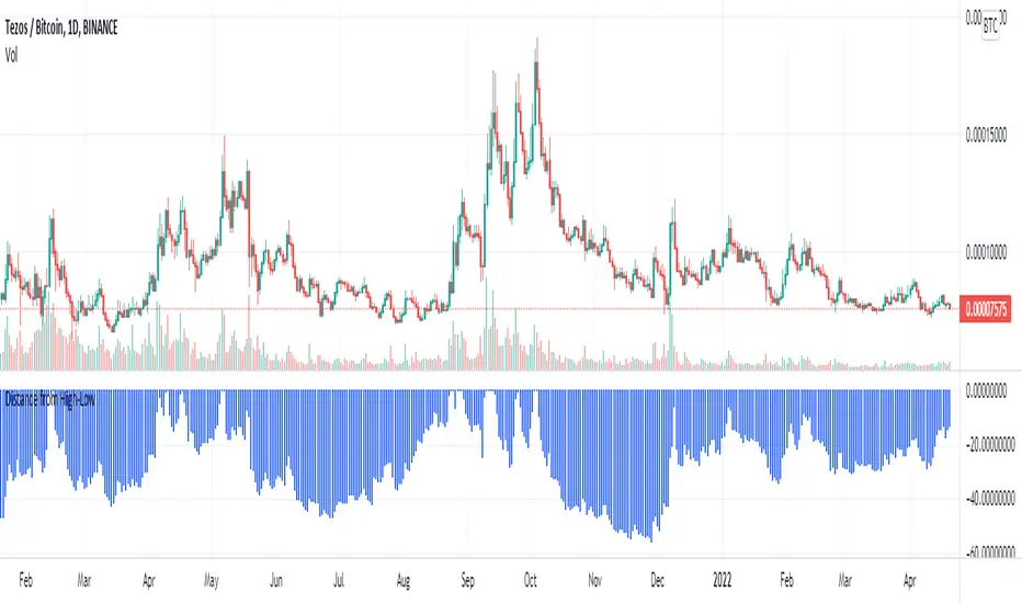
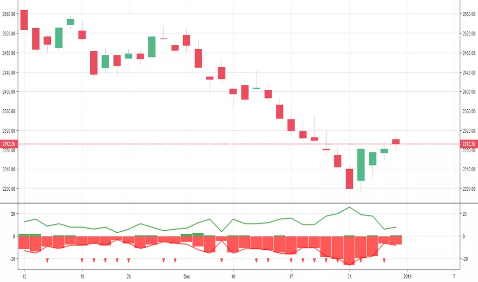
Distance/Drawdown from a period high/lowShow distance (%) from previous high/low in selected period.Pine Script®指标由Cryptauk提供已更新 2235
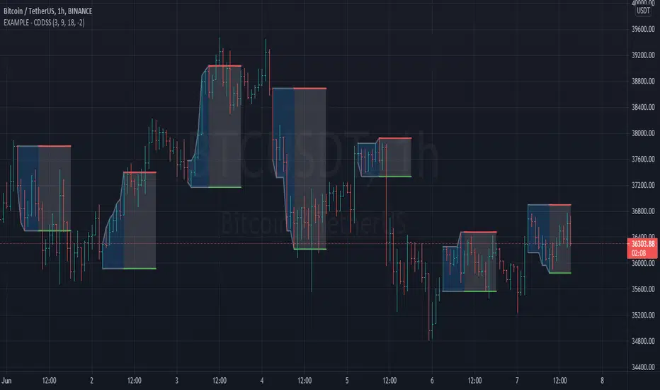
Same high/low + DCA (only long)This is an update of the previous "same high/low" strategy. This strategy can be helpful for those who look for entrance price points after level retest based on the dollar cost averaging approach. The retest of the level is defined by two candles with the same low. 4 entrance points were calculated based on volatility (not based on ATR though) and the weights were averaged in the middle of the volatility level. As previously, stop loss is just one tick away from a level of support and take profit based on the ATR multiplier. Pine Script®策略由Cherepanov_V提供22164
Percentage Levels by TimeframePlots the positive and negative percentage levels from a selection of timeframes and sources for any ticker. You can use this within a pullback trading system. For example, if you historically look at the average pullback of large cap stocks and ETF's, you can use this indicator to plot the levels it could pullback to for an entry to go long. It can be used as potential targets when trading a ticker short. Another use for this is to backtest the set percentage targets using TradingView's bar replay feature to see how ETF's and large cap stocks have reacted at these levels. Note: This is intended to be used at timeframes equal to higher than the chart's as it may cause re-painting issues. Currently percentage levels are statically set to 1, 3, 5, 10, 15, 20, 25, and 30% levels above and below the chosen source (open, high, low, close). You can also display the data based on timeframes from Daily (1D) all the way up to Yearly (12M) *Not financial advice but in my opinion the current percentage levels set (see above) are best used for ETF's and Large Cap Stocks. Jan 2 Release Notes: Added the ability to select the historical bars to look back when plotting levels Jan 2 Release Notes: To get a better display or proper resolution on your charts, change the view settings to "Scale Price Chart Only" Jan 2 Release Notes: To add % labels for this indicator on the price axis, change your chart settings to include "Indicator Name Label" & "Indicator Last Value". You can find this under the Label section after hitting the gear icon in the bottom right of your chart. Jan 2 Release Notes: Added: Custom Line Plot Extension Settings. Ideally both values should be equal to display optimal extended lines. To return to a base setting: '1' = Historical Lookback & '0' = Offset Lines. Also note this is dependent on the timeframe you are viewing on the chart. Jan 2 Release Notes: Removed indicator from example chart that was not needed. Jan 2 Release Notes: Updated some comments in the Pine Script Jan 2 Release Notes: Update: Added commentary and instructions in the indicator settings to address recommended line plot settings for Stocks/ETF's vs Futures Jan 2 Release Notes: Changed title from "Calculation Method" to "Calculation Source" Jan 4 2021 Normal use of security() dictates that it only be used at timeframes equal to or higher than the chart's as it may cause re-paintingPine Script®指标由thacoolbreeze提供已更新 44242
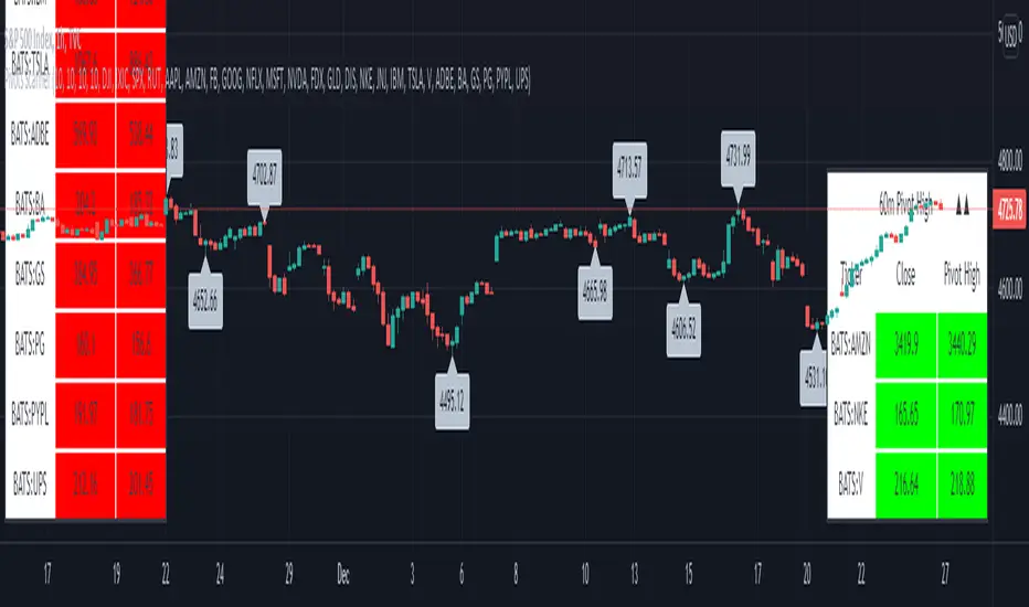
Pivots High-Low Screener & AlertsHi fellow traders , Pleased to share a Pivot High - Low Screener. The script uses the TV inbuilt Pivot function. It Screens 25 tickers default set, these can be modified in the input dialog box. All you need to do is attach to any chart and set the periodicity or the resolution of the chart to your desired alert() frequency requirement. Now go to the input settings icon of the script and set your Pivot right and left parameters! Set the alert from the menu as usual click - Any alert() function call and bingo you are done!! Similarily change the chart periodicity to the next timeframe and set the next alert. No more opening multiple charts and setting individual time consuming alerts(). You will get concatenated alerts or summary alerts for your tickers. Track 25tickers with a single alert for each timeframe(Supports 40 tickers). Happy trading with TV.. Pine Script®指标由sharaaU7提供1212474
Gann High Low Activator AlertsA Gann High Low Activator within a fixed range meant for alerts. A value of 1 means we're in an uptrend, a value of -1 a downtrend, and a value of 0 is neutral. Thank you and happy tradingPine Script®指标由jaNGOB提供83
Example - Custom Defined Dual-State SessionThis script example aims to cover the following: defining custom timeframe / session windows gather a price range from the custom period ( high/low values ) create a secondary "holding" period through which to display the data collected from the initial session simple method to shift times to re-align to preferred timezone Articles and further reading: www.investopedia.com - trading session Reason for Study: Educational purposes only. Before considering writing this example I had seen multiple similar questions asking how to go about creating custom timeframes or sessions, so it seemed this might be a good topic to attempt to create a relatively generic example.Pine Script®指标由JayRogers提供已更新 1616449
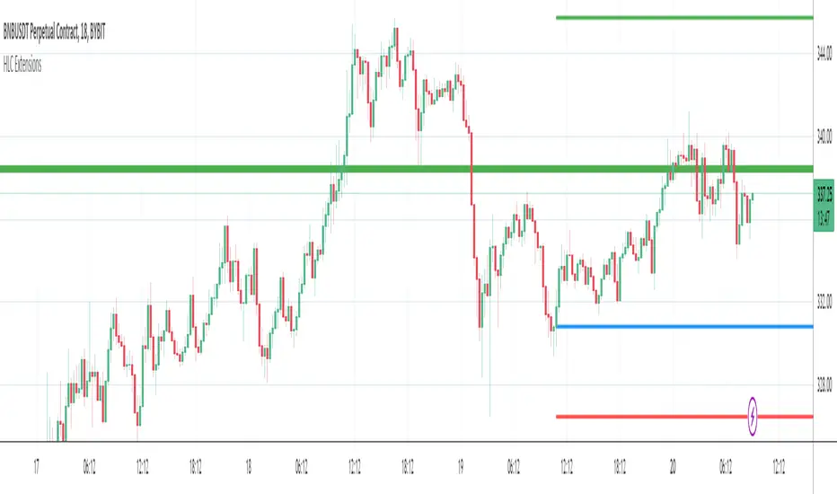
Yesterdays & Last Weeks High Low Close ExtensionsPlots the Extensions of Yesterdays and Last Weeks High Low Close Unfortunately all of the levels wont always show therefore it is good use this in conjunction with my Levels script I tried to combine the 2 scripts but doing so gave me memory overload errors in Tradingview thats why I have made them separatePine Script®指标由Lij_MC提供已更新 99553
Open/High/Low/Close (OHLC) Lines with Configurable TimeframeThis script draws open/high/low/close (OHLC) lines for the previous bar from the configured timeframe. This enables you to use higher timeframes, like a daily chart and OHLC lines of the previous week.Pine Script®指标由Me_On_Vacation提供已更新 77452
Yesterday HLOC and Two days High low open closeYesterday HLOC and Two days High low open closePine Script®指标由anand6878提供55328
Yearly OHLplots Yearly Open, High, Low levels Interesting interactions to note at previous yearly opensPine Script®指标由Chonky_提供158
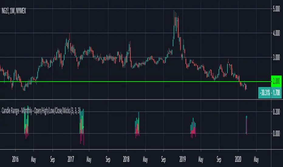
Candle Range - Monthly - Open/High/Low/Close/Wicks (Oldinvestor)This candle range comparison is similar to my original script Candle Range Compare . This script is to compares the size of open/close high/low and wick size side by side. This version of the script allows you to only show a chosen month of each year to compare. I hadn't even thought to try and vanish the part of the chart I'm not looking at. I'll consider that later (may never happen, I am limited on time). I have also included check boxes to turn on/off certain candles. This part is pretty self explanatory. For example: if you wish to not see wicks in front of the open/close, go to the settings for the study and uncheck the box for "Show Wicks". Warning: The script does not work so well on monthly candles? Some of the candles are missing... Good luck Oldinvestor Pine Script®指标由oldinvestor提供22122
anas MACD high low div conv trying to detect divergent and using high low in MACDPine Script®指标由anashassan76提供41
Custom Time ranges. Daily price ranges.Addition to previous time range script, now containing daily ranges. You can select a day of the week, and have it show the high, low, mid, and open of that day. For the time bands: Monday = 2 Tuesday = 3 Wednesday = 4 Thursday = 5 Friday = 6 Saturday = 7 Sunday = 1 Example 1: 1500-1800:2 This will colour the background between 3pm and 6pm on Mondays. Example 2: 0000-0600:247 This will colour the background between midnight and 6am on Mondays, Wednesdays, and Saturdays. For the Daily price ranges: Just select the tick-box forthe day, and then the price levels you'd like to see. I want to add specific weekly levels to this, for example: week 06 of year 2020, but I've not figured out how to do it yet. If anyone knows, I'd appreciate it if you let me know. I'll then update this script. As always, any questions you may have, please leave in comments below and I'll respond when I have time. If you notice anything good with this indicator, let me know. We are all in this to make money after all! ;)Pine Script®指标由Plumptoiletduck提供1919367
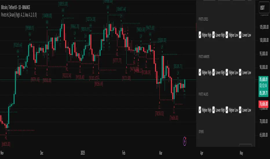
Pivot Points High Low (HH/HL/LH/LL) [Anan]Hello Friends, This is my own version of ( Pivot Hilo Support n Resistance Levels R3-3 by JustUncleL ) - V4 Pinescript - Removed MA dependency filters - Add some arrows Pine Script®指标由Mohamed3nan提供已更新 5555 5 K
Previous OHLC LevelsQuick dirty code for personal use. Plots previous OHLC levels based on a selected time-frame on the chart. Not bad if you want to see different time-frame levels. Fill function can serve to highlight the daily range (high-low or open-close) on non-standard charts Uses base code from JayRogersPine Script®指标由kewbimingle提供11546
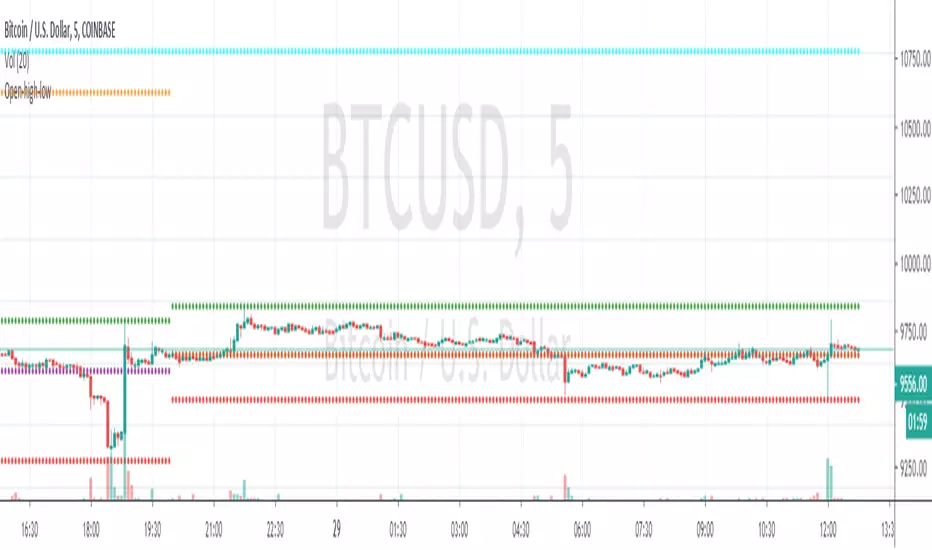
Open-high-lowmodified @traderXO's original daily open/high/low script to include monthly and weekly open.Pine Script®指标由CryptoRogue提供11105
Standard Deviation using high, low, closeEvery standard deviation tools just only consider one source to compute std, but this tool also consider close, high, low to publish stdPine Script®指标由dastmard提供54
Pivot High Low Pointsby using this script you can find Pivot High-Low Points. This script works like Tradingview pivothigh & pivotlow functions. If you find my works useful, please consider a donation BTC: 16XRqyS3Vgh1knAU1tCcruqhUrVm4QWWmR by LonesomeTheBlue Pine Script®指标由LonesomeTheBlue提供已更新 3030 1.9 K
Current Open/Previous High Low Close. Gap HighlightedThis script plots the current open previous high low close. Also the area between the current open and previous close are highlighted to easily see the overnight gap. The idea is that after a significant gap the price will retest previous days levels before continuing in the direction of the gap.Pine Script®指标由Craig_Stine提供11246
New Highs-Lows AMEX-Buschi English: This indicator shows the AMEX's up volume (green) and down volume (red). Extreme trading days with more than 90 % up or down volume are marked via lines (theoretically values) and triangles (breaches). Deutsch: Dieser Indikator zeigt das Aufwärts- (grün) und Abwärts-Volumen (rot) der AMEX. Extreme Handelstage mit mehr als 90 % Aufwärts- oder Abwärts-Volumen ist gekennzeichnet über Linien (theoretische Werte) und Dreiecke (Überschreitungen).Pine Script®指标由MagicEins提供已更新 44213
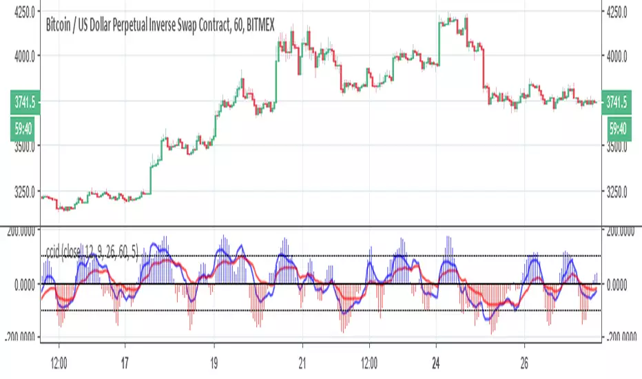
ccid (with high low histogram)So this indicator has the following : CCI where the buy and sell signal can be either cross of the fast the slow and vice versa or cross of CCI bellow -50 and cross down CCI +50 the histogram (blue and red) is made by high low like histogram the buy and sell is based on crossing of the 0 . since its MTF type . you can toon the TF either to the time frame or use lower graph time with higher TF since both indicator complement each other then I put them together Pine Script®指标由RafaelZioni提供61
Previous 2Days High/LowTesting simple range of highs/lows of previous 2 days, for reference, working on every timeframe.Pine Script®指标由Wingman提供已更新 66333