DCA After Downtrend v2 (by BHD_Trade_Bot)The purpose of the strategy is to identify the end of a short-term downtrend . So that you can easily to DCA certain amount of money for each month.
ENTRY
The buy orders are placed on a monthly basis for assets at the end of a short-term downtrend:
- Each month condition: In 1-hour time frame, each month has 24 * 30 candles
- The end of short-term downtrend condition: use MACD for less delay
CLOSE
The sell orders are placed when:
- Is last bar
The strategy use $1000 and trading fee is 1.1% for each order.
Pro tip: The 1-hour time frame has the best results on average:
- Total spent: $1000 x 33 = $33,000
- Total profit: $65,578
在脚本中搜索"油价调整最新消息:国内油价今日24时上调多少"

Jathuko Boncu Serok Cendolserok brrooo....
Jakarta - Celsius Network LLC menggugat mantan manajer investasinya, Jason Stone pada selasa lalu. Perusahaan pemberi pinjaman kripto ini menuduh Stone mencuri aset puluhan juta dolar sebelum bangkrut bulan lalu.
Dalam pengaduan yang diajukan di pengadilan kebangkrutan Manhattan, Celsius menuduh Stone dan perusahaannya KeyFi Inc melakukan kelalaian fatal. Stone juga dituduh tidak berkompeten dalam berinvestasi kripto.
Dikutip dari Reuters, Rabu (24/8/2022), Celsius mengatakan Stone terbukti gagal memberikan untung dan menyebabkan kerugian puluhan juta dolar.
Baca artikel detikfinance, "Diduga Tilep Kripto Puluhan Juta Dolar, Manajer Ini Digugat Perusahaannya" selengkapnya

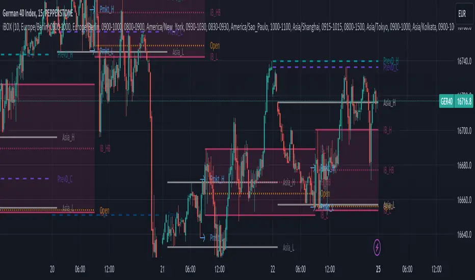
iBox, Initial Balance | IB High, Low, Midpoint | OpeningThis Indicator will print basically 4 lines.
You have to understand the importance of the "Initial Balance" the first trading hour of Cash session is very important in trading stocks and indizes.
So you will get 4 lines:
Opening
Initial Balance High
Initial Balance Low
Initial Balance Midpoint/Halfback
Most indicators for Range Box, Opening Trade, Opening Range, Initial Balance, iBOX and "Ultimate Lines" will only use the timezone of the exchange or your own timezone. I'm living in europe and we have this daylight saving time change in Summer/Winter - which will cause problems with most of the existing indicators or at least will push you to change the times regularly.
Another important point: I really like to switch the indizes when trading on my mobile. So what will happen when you set up opening range for DAX at 09:00 and then switch to S&P500? All indicators I tried failed here - they will just draw a wrong line for SPX, NDX, DJI, FTSE, ASX etc. I fixed that and hard coded stock exchanges and ticker symbols into 3 main groups Initial Balance EU/US/Asia
For example we take DAX - XETRA DAX is opening at 09:00 MEZ (Europe/Berlin)
The Initial Balance is set during the H1 Candle from 09:00 - 09:59
Please be aware, that some cash indizes only deliver data to TradingView after the "opening auction" - so for Xetra DAX you have to book live data and often you will only see data at 09:02/09:03 after the opening auction.
So you will get different opening lines compared from cash to future or your CFD provider. Future and CFD should fit for 99%
The Opening Line will be drawn at exactly 09:00
IB High on the highest price during the H1 candle
IB Low on the lowest price during the H1 candle
IB Halfback is simple: (IB High + IB Low) / 2
The lines will be drawn from cash start until next day and will end 2 minutes before the next cash session will start again. Please make your own experience! Activate the indicator for a CFD or Future switch to M15 and watch the wicks around the 4 lines. Even in the night or the next morning before the next Initial Balance will be set.
For me the lines are valid for around 24 hours and often longer. That's why it's good to have the old lines on the chart too.
To-do:
Yesterday high / low / close / halfback (also for last week and month)
Labels for the lines - sometimes only the colors will confuse you - a simple label should be a benefit (IB_h, IB_l, IB_1/2, 1D_o)
Range Lines for Asia Range and Premarket Range - additionaly a parameter to disable premarket lines when premarket is trading in asia range.
Add Alert condition to get alerts after IB is set
If you have and thoughts, ideas or improvements, please send me an message or leave an comment!
Like i said, the stock exchanges and ticker symbols are hard coded and can be extended for all relevant assets.
Have fun and i really hope this indicator will help improving your trading experience!
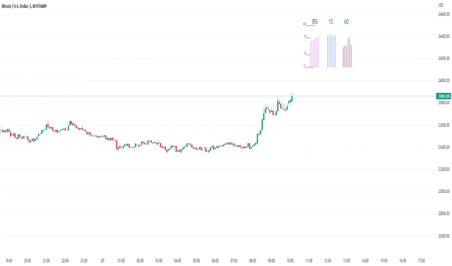
Rsi/W%R/Stoch/Mfi: HTF overlay mini-plotsOverlay mini-plots for various indicators. Shows current timeframe; and option to plot 2x higher timeframes (i.e. 15min and 60min on the 5min chart above).
The idea is to de-clutter chart when you just want real-time snippets for an indicator.
Useful for gauging overbought/oversold, across timeframes, at a glance.
~~Indicators~~
~RSI: Relative strength index
~W%R: Williams percent range
~Stochastic
~MFI: Money flow index
~~Inputs~~
~indicator length (NB default is set to 12, NOT the standard 14)
~choose 2x HTFs, show/hide HTF plots
~choose number of bars to show (current timeframe only; HTF plots show only 6 bars)
~horizontal position: offset (bars); shift plots right or left. Can be negative
~vertical position: top/middle/bottom
~other formatting options (color, line thickness, show/hide labels, 70/30 lines, 80/20 lines)
~~tips~~
~should be relatively easy to add further indicators, so long as they are 0-100 based; by editing lines 9 and 11
~change the vertical compression of the plots by playing around with the numbers (+100, -400, etc) in lines 24 and 25
Normalized, Variety, Fast Fourier Transform Explorer [Loxx]Normalized, Variety, Fast Fourier Transform Explorer demonstrates Real, Cosine, and Sine Fast Fourier Transform algorithms. This indicator can be used as a rule of thumb but shouldn't be used in trading.
What is the Discrete Fourier Transform?
In mathematics, the discrete Fourier transform (DFT) converts a finite sequence of equally-spaced samples of a function into a same-length sequence of equally-spaced samples of the discrete-time Fourier transform (DTFT), which is a complex-valued function of frequency. The interval at which the DTFT is sampled is the reciprocal of the duration of the input sequence. An inverse DFT is a Fourier series, using the DTFT samples as coefficients of complex sinusoids at the corresponding DTFT frequencies. It has the same sample-values as the original input sequence. The DFT is therefore said to be a frequency domain representation of the original input sequence. If the original sequence spans all the non-zero values of a function, its DTFT is continuous (and periodic), and the DFT provides discrete samples of one cycle. If the original sequence is one cycle of a periodic function, the DFT provides all the non-zero values of one DTFT cycle.
What is the Complex Fast Fourier Transform?
The complex Fast Fourier Transform algorithm transforms N real or complex numbers into another N complex numbers. The complex FFT transforms a real or complex signal x in the time domain into a complex two-sided spectrum X in the frequency domain. You must remember that zero frequency corresponds to n = 0, positive frequencies 0 < f < f_c correspond to values 1 ≤ n ≤ N/2 −1, while negative frequencies −fc < f < 0 correspond to N/2 +1 ≤ n ≤ N −1. The value n = N/2 corresponds to both f = f_c and f = −f_c. f_c is the critical or Nyquist frequency with f_c = 1/(2*T) or half the sampling frequency. The first harmonic X corresponds to the frequency 1/(N*T).
The complex FFT requires the list of values (resolution, or N) to be a power 2. If the input size if not a power of 2, then the input data will be padded with zeros to fit the size of the closest power of 2 upward.
What is Real-Fast Fourier Transform?
Has conditions similar to the complex Fast Fourier Transform value, except that the input data must be purely real. If the time series data has the basic type complex64, only the real parts of the complex numbers are used for the calculation. The imaginary parts are silently discarded.
What is the Real-Fast Fourier Transform?
In many applications, the input data for the DFT are purely real, in which case the outputs satisfy the symmetry
X(N-k)=X(k)
and efficient FFT algorithms have been designed for this situation (see e.g. Sorensen, 1987). One approach consists of taking an ordinary algorithm (e.g. Cooley–Tukey) and removing the redundant parts of the computation, saving roughly a factor of two in time and memory. Alternatively, it is possible to express an even-length real-input DFT as a complex DFT of half the length (whose real and imaginary parts are the even/odd elements of the original real data), followed by O(N) post-processing operations.
It was once believed that real-input DFTs could be more efficiently computed by means of the discrete Hartley transform (DHT), but it was subsequently argued that a specialized real-input DFT algorithm (FFT) can typically be found that requires fewer operations than the corresponding DHT algorithm (FHT) for the same number of inputs. Bruun's algorithm (above) is another method that was initially proposed to take advantage of real inputs, but it has not proved popular.
There are further FFT specializations for the cases of real data that have even/odd symmetry, in which case one can gain another factor of roughly two in time and memory and the DFT becomes the discrete cosine/sine transform(s) (DCT/DST). Instead of directly modifying an FFT algorithm for these cases, DCTs/DSTs can also be computed via FFTs of real data combined with O(N) pre- and post-processing.
What is the Discrete Cosine Transform?
A discrete cosine transform ( DCT ) expresses a finite sequence of data points in terms of a sum of cosine functions oscillating at different frequencies. The DCT , first proposed by Nasir Ahmed in 1972, is a widely used transformation technique in signal processing and data compression. It is used in most digital media, including digital images (such as JPEG and HEIF, where small high-frequency components can be discarded), digital video (such as MPEG and H.26x), digital audio (such as Dolby Digital, MP3 and AAC ), digital television (such as SDTV, HDTV and VOD ), digital radio (such as AAC+ and DAB+), and speech coding (such as AAC-LD, Siren and Opus). DCTs are also important to numerous other applications in science and engineering, such as digital signal processing, telecommunication devices, reducing network bandwidth usage, and spectral methods for the numerical solution of partial differential equations.
The use of cosine rather than sine functions is critical for compression, since it turns out (as described below) that fewer cosine functions are needed to approximate a typical signal, whereas for differential equations the cosines express a particular choice of boundary conditions. In particular, a DCT is a Fourier-related transform similar to the discrete Fourier transform (DFT), but using only real numbers. The DCTs are generally related to Fourier Series coefficients of a periodically and symmetrically extended sequence whereas DFTs are related to Fourier Series coefficients of only periodically extended sequences. DCTs are equivalent to DFTs of roughly twice the length, operating on real data with even symmetry (since the Fourier transform of a real and even function is real and even), whereas in some variants the input and/or output data are shifted by half a sample. There are eight standard DCT variants, of which four are common.
The most common variant of discrete cosine transform is the type-II DCT , which is often called simply "the DCT". This was the original DCT as first proposed by Ahmed. Its inverse, the type-III DCT , is correspondingly often called simply "the inverse DCT" or "the IDCT". Two related transforms are the discrete sine transform ( DST ), which is equivalent to a DFT of real and odd functions, and the modified discrete cosine transform (MDCT), which is based on a DCT of overlapping data. Multidimensional DCTs ( MD DCTs) are developed to extend the concept of DCT to MD signals. There are several algorithms to compute MD DCT . A variety of fast algorithms have been developed to reduce the computational complexity of implementing DCT . One of these is the integer DCT (IntDCT), an integer approximation of the standard DCT ,: ix, xiii, 1, 141–304 used in several ISO /IEC and ITU-T international standards.
What is the Discrete Sine Transform?
In mathematics, the discrete sine transform (DST) is a Fourier-related transform similar to the discrete Fourier transform (DFT), but using a purely real matrix. It is equivalent to the imaginary parts of a DFT of roughly twice the length, operating on real data with odd symmetry (since the Fourier transform of a real and odd function is imaginary and odd), where in some variants the input and/or output data are shifted by half a sample.
A family of transforms composed of sine and sine hyperbolic functions exists. These transforms are made based on the natural vibration of thin square plates with different boundary conditions.
The DST is related to the discrete cosine transform (DCT), which is equivalent to a DFT of real and even functions. See the DCT article for a general discussion of how the boundary conditions relate the various DCT and DST types. Generally, the DST is derived from the DCT by replacing the Neumann condition at x=0 with a Dirichlet condition. Both the DCT and the DST were described by Nasir Ahmed T. Natarajan and K.R. Rao in 1974. The type-I DST (DST-I) was later described by Anil K. Jain in 1976, and the type-II DST (DST-II) was then described by H.B. Kekra and J.K. Solanka in 1978.
Notable settings
windowper = period for calculation, restricted to powers of 2: "16", "32", "64", "128", "256", "512", "1024", "2048", this reason for this is FFT is an algorithm that computes DFT (Discrete Fourier Transform) in a fast way, generally in 𝑂(𝑁⋅log2(𝑁)) instead of 𝑂(𝑁2). To achieve this the input matrix has to be a power of 2 but many FFT algorithm can handle any size of input since the matrix can be zero-padded. For our purposes here, we stick to powers of 2 to keep this fast and neat. read more about this here: Cooley–Tukey FFT algorithm
SS = smoothing count, this smoothing happens after the first FCT regular pass. this zeros out frequencies from the previously calculated values above SS count. the lower this number, the smoother the output, it works opposite from other smoothing periods
Fmin1 = zeroes out frequencies not passing this test for min value
Fmax1 = zeroes out frequencies not passing this test for max value
barsback = moves the window backward
Inverse = whether or not you wish to invert the FFT after first pass calculation
Related indicators
Real-Fast Fourier Transform of Price Oscillator
STD-Stepped Fast Cosine Transform Moving Average
Real-Fast Fourier Transform of Price w/ Linear Regression
Variety RSI of Fast Discrete Cosine Transform
Additional reading
A Fast Computational Algorithm for the Discrete Cosine Transform by Chen et al.
Practical Fast 1-D DCT Algorithms With 11 Multiplications by Loeffler et al.
Cooley–Tukey FFT algorithm
Ahmed, Nasir (January 1991). "How I Came Up With the Discrete Cosine Transform". Digital Signal Processing. 1 (1): 4–5. doi:10.1016/1051-2004(91)90086-Z.
DCT-History - How I Came Up With The Discrete Cosine Transform
Comparative Analysis for Discrete Sine Transform as a suitable method for noise estimation

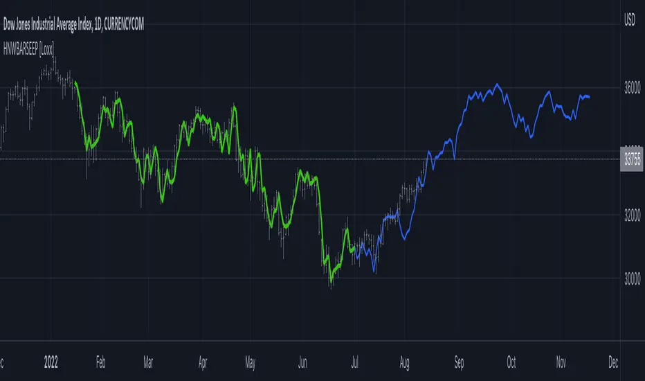
Helme-Nikias Weighted Burg AR-SE Extra. of Price [Loxx]Helme-Nikias Weighted Burg AR-SE Extra. of Price is an indicator that uses an autoregressive spectral estimation called the Weighted Burg Algorithm, but unlike the usual WB algo, this one uses Helme-Nikias weighting. This method is commonly used in speech modeling and speech prediction engines. This is a linear method of forecasting data. You'll notice that this method uses a different weighting calculation vs Weighted Burg method. This new weighting is the following:
w = math.pow(array.get(x, i - 1), 2), the squared lag of the source parameter
and
w += math.pow(array.get(x, i), 2), the sum of the squared source parameter
This take place of the rectangular, hamming and parabolic weighting used in the Weighted Burg method
Also, this method includes Levinson–Durbin algorithm. as was already discussed previously in the following indicator:
Levinson-Durbin Autocorrelation Extrapolation of Price
What is Helme-Nikias Weighted Burg Autoregressive Spectral Estimate Extrapolation of price?
In this paper a new stable modification of the weighted Burg technique for autoregressive (AR) spectral estimation is introduced based on data-adaptive weights that are proportional to the common power of the forward and backward AR process realizations. It is shown that AR spectra of short length sinusoidal signals generated by the new approach do not exhibit phase dependence or line-splitting. Further, it is demonstrated that improvements in resolution may be so obtained relative to other weighted Burg algorithms. The method suggested here is shown to resolve two closely-spaced peaks of dynamic range 24 dB whereas the modified Burg schemes employing rectangular, Hamming or "optimum" parabolic windows fail.
Data inputs
Source Settings: -Loxx's Expanded Source Types. You typically use "open" since open has already closed on the current active bar
LastBar - bar where to start the prediction
PastBars - how many bars back to model
LPOrder - order of linear prediction model; 0 to 1
FutBars - how many bars you want to forward predict
Things to know
Normally, a simple moving average is calculated on source data. I've expanded this to 38 different averaging methods using Loxx's Moving Avreages.
This indicator repaints
Further reading
A high-resolution modified Burg algorithm for spectral estimation
Related Indicators
Levinson-Durbin Autocorrelation Extrapolation of Price
Weighted Burg AR Spectral Estimate Extrapolation of Price
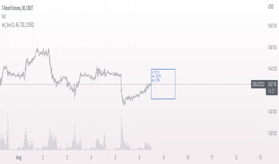
vol_boxA simple script to draw a realized volatility forecast, in the form of a box. The script calculates realized volatility using the EWMA method, using a number of periods of your choosing. Using the "periods per year", you can adjust the script to work on any time frame. For example, if you are using an hourly chart with bitcoin, there are 24 periods * 365 = 8760 periods per year. This setting is essential for the realized volatility figure to be accurate as an annualized figure, like VIX.
By default, the settings are set to mimic CBOE volatility indices. That is, 252 days per year, and 20 period window on the daily timeframe (simulating a 30 trading day period).
Inside the box are three figures:
1. The current realized volatility.
2. The rank. E.g. "10%" means the current realized volatility is less than 90% of realized volatility measures.
3. The "accuracy": how often price has closed within the box, historically.
Inputs:
stdevs: the number of standard deviations for the box
periods to project: the number of periods to forecast
window: the number of periods for calculating realized volatility
periods per year: the number of periods in one year (e.g. 252 for the "D" timeframe)
FOMC AnnouncementsThis indicator plots vertical lines at the scheduled times of US Federal Reserve's FOMC Meeting Announcements. Usually, that time or the 24 hours before and after could see big moves in markets. You can change those dates and times in the settings, and could use the indicator option "Add this indicator to entire layout" if you want to easily reflect that across all panes of a layout. Those lines will show on any symbol you switch to, saving you time and effort of drawing them manually.

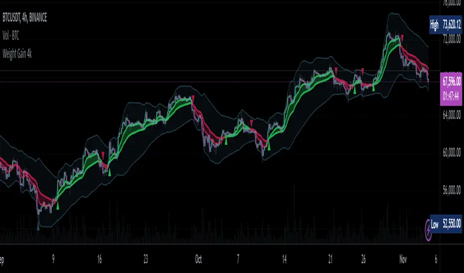
Weight Gain 4000 - (Adjustable Volume Weighted MA) - [mutantdog]Short Version:
This is a fairly self-contained system based upon a moving average crossover with several unique features. The most significant of these is the adjustable volume weighting system, allowing for transformations between standard and weighted versions of each included MA. With this feature it is possible to apply partial weighting which can help to improve responsiveness without dramatically altering shape. Included types are SMA, EMA, WMA, RMA, hSMA, DEMA and TEMA. Potentially more will be added in future (check updates below).
In addition there are a selection of alternative 'weighted' inputs, a pair of Bollinger-style deviation bands, a separate price tracker and a bunch of alert presets.
This can be used out-of-the-box or tweaked in multiple ways for unusual results. Default settings are a basic 8/21 EMA cross with partial volume weighting. Dev bands apply to MA2 and are based upon the type and the volume weighting. For standard Bollinger bands use SMA with length 20 and try adding a small amount of volume weighting.
A more detailed breakdown of the functionality follows.
Long Version:
ADJUSTABLE VOLUME WEIGHTING
In principle any moving average should have a volume weighted analogue, the standard VWMA is just an SMA with volume weighting for example. Actually, we can consider the SMA to be a special case where volume is a constant 1 per bar (the value is somewhat arbitrary, the important part is that it's constant). Similar principles apply to the 'elastic' EVWMA which is the volume weighted analogue of an RMA. In any case though, where we have standard and weighted variants it is possible to transform one into the other by gradually increasing or decreasing the weighting, which forms the basis of this system. This is not just a simple multiplier however, that would not work due to the relative proportions being the same when set at any non zero value. In order to create a meaningful transformation we need to use an exponent instead, eg: volume^x , where x is a variable determined in this case by the 'volume' parameter. When x=1, the full volume weighting applies and when x=0, the volume will be reduced to a constant 1. Values in between will result in the respective partial weighting, for example 0.5 will give the square root of the volume.
The obvious question here though is why would you want to do this? To answer that really it is best to actually try it. The advantages that volume weighting can bring to a moving average can sometimes come at the cost of unwanted or erratic behaviour. While it can tend towards much closer price tracking which may be desirable, sometimes it needs moderating especially in markets with lower liquidity. Here the adjustability can be useful, in many cases i have found that adding a small amount of volume weighting to a chosen MA can help to improve its responsiveness without overpowering it. Another possible use case would be to have two instances of the same MA with the same length but different weightings, the extent to which these diverge from each other can be a useful indicator of trend strength. Other uses will become apparent with experimentation and can vary from one market to another.
THE INCLUDED MODES
At the time of publication, there are 7 included moving average types with plans to add more in future. For now here is a brief explainer of what's on offer (continuing to use x as shorthand for the volume parameter), starting with the two most common types.
SMA: As mentioned above this is essentially a standard VWMA, calculated here as sma(source*volume^x,length)/sma(volume^x,length). In this case when x=0 then volume=1 and it reduces to a standard SMA.
RMA: Again mentioned above, this is an EVWMA (where E stands for elastic) with constant weighting. Without going into detail, this method takes the 1/length factor of an RMA and replaces it with volume^x/sum(volume^x,length). In this case again we can see that when x=0 then volume=1 and the original 1/length factor is restored.
EMA: This follows the same principle as the RMA where the standard 2/(length+1) factor is replaced with (2*volume^x)/(sum(volume^x,length)+volume^x). As with an RMA, when x=0 then volume=1 and this reduces back to the standard 2/(length+1).
DEMA: Just a standard Double EMA using the above.
TEMA: Likewise, a standard Triple EMA using the above.
hSMA: This is the same as the SMA except it uses harmonic mean calculations instead of arithmetic. In most cases the differences are negligible however they can become more pronounced when volume weighting is introduced. Furthermore, an argument can be made that harmonic mean calculations are better suited to downtrends or bear markets, in principle at least.
WMA: Probably the most contentious one included. Follows the same basic calculations as for the SMA except uses a WMA instead. Honestly, it makes little sense to combine both linear and volume weighting in this manner, included only for completeness and because it can easily be done. It may be the case that a superior composite could be created with some more complex calculations, in which case i may add that later. For now though this will do.
An additional 'volume filter' option is included, which applies a basic filter to the volume prior to calculation. For types based around the SMA/VWMA system, the volume filter is a WMA-4, for types based around the RMA/EVWMA system the filter is a RMA-2.
As and when i add more they will be listed in the updates at the bottom.
WEIGHTED INPUTS
The ohlc method of source calculations is really a leftover from a time when data was far more limited. Nevertheless it is still the method used in charting and for the most part is sufficient. Often the only important value is 'close' although sometimes 'high' and 'low' can be relevant also. Since we are volume weighting however, it can be useful to incorporate as much information as possible. To that end either 'hlc3' or 'hlcc4' tend to be the best of the defaults (in the case of 24/7 charting like crypto or intraday trading, 'ohlc4' should be avoided as it is effectively the same as a lagging version of 'hlcc4'). There are many other (infinitely many, in fact) possible combinations that can be created, i have included a few here.
The premise is fairly straightforward, by subtracting one value from another, the remaining difference can act as a kind of weight. In a simple case consider 'hl2' as simply the midrange ((high+low)/2), instead of this using 'high+low-open' would give more weight to the value furthest from the open, providing a good estimate of the median. An even better estimate can be achieved by combining that with 'high+low-close' to give the included result 'hl-oc2'. Similarly, 'hlc3' can be considered the basic mean of the three significant values, an included weighted version 'hlc2-o2' combines a sum with subtraction of open to give an estimated mean that may be more accurate. Finally we can apply a similar principle to the close, by subtracting the other values, this one potentially gets more complex so the included 'cc-ohlc4' is really the simplest. The result here is an overbias of the close in relation to the open and the midrange, while in most cases not as useful it can provide an estimate for the next bar assuming that the trend continues.
Of the three i've included, hlc2-o2 is in my opinion the most useful especially in this context, although it is perhaps best considered to be experimental in nature. For that reason, i've kept 'hlcc4' as the default for both MAs.
Additionally included is an 'aux input' which is the standard TV source menu and, where possible, can be set as outputs of other indicators.
THE SYSTEM
This one is fairly obvious and straightforward. It's just a moving average crossover with additional deviation (bollinger) bands. Not a lot to explain here as it should be apparent how it works.
Of the two, MA1 is considered to be the fast and MA2 is considered to be the slow. Both can be set with independent inputs, types and weighting. When MA1 is above, the colour of both is green and when it's below the colour of both is red. An additional gradient based fill is there and can be adjusted along with everything else in the visuals section at the bottom. Default alerts are available for crossover/crossunder conditions along with optional marker plots.
MA2 has the option for deviation bands, these are calculated based upon the MA type used and volume weighted according to the main parameter. In the case of a unweighted SMA being used they will be standard Bollinger bands.
An additional 'source direct' price tracker is included which can be used as the basis for an alert system for price crossings of bands or MAs, while taking advantage of the available weighted inputs. This is displayed as a stepped line on the chart so is also a good way to visualise the differences between input types.
That just about covers it then. The likelihood is that you've used some sort of moving average cross system before and are probably still using one or more. If so, then perhaps the additional functionality here will be of benefit.
Thanks for looking, I welcome any feedack
ka66: Auto-Guppy Multiple Moving Average (GMMA)This implements a Guppy Multiple Moving Average (GMMA) with the following twists, which may be a feature or a bug, depending on your perspective:
For both fast and slow group of MAs, only a starting MA (the fastest in that group) is specified.
For either group, a configurable factor is set, which will be used to calculate subsequent MAs.
Automatically selects colours as gradients within a configurable colour range, clearly differentiating between the short-term and long-term groups of averages.
Use Weighted Moving Average (WMAs) as the averaging mechanism. More on this later.
For example, if in the fast group, we start with MA 3, and a factor of 2, then the 6 MAs in the group will be: 3, 6, 12, 24, 48, 96.
The calculated lookbacks are displayed on a table on the top-right, in case further indicators need to be calculated based on these values.
Use of WMAs : This is an annoyance of the implementation: As I use arrays to store lookback calculations (12 of them, individual variables would be a pani to work with!), getting these back out of the array returns a series rather than a simple value. For some unfathomable reason, PineScript doesn't allow copying/conversion of these into a simple value. To add insult to the injury, a bunch of moving averaging functions (e.g.: ta.ema, ta.hma) only work with simple int lookback values. Go figure. SMAs and WMAs are the two that allow series lookback values, and WMAs are less laggy than SMAs but remain smooth, so WMAs it is!

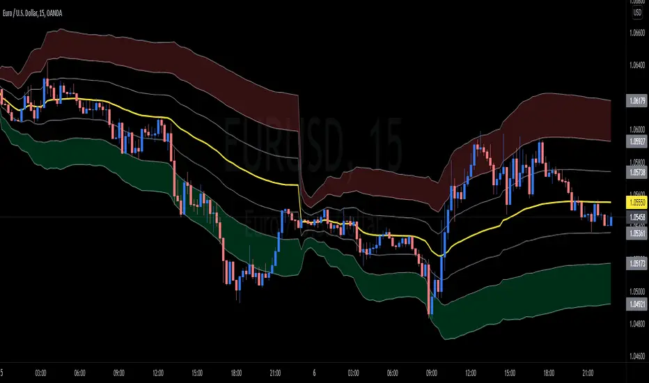
SigmaSpikes Background Highlight [vnhilton]SigmaSpikes is an indicator created by Adam H Grimes. It's a volatility indicator which applies a standard deviation measure on candles for a set period of time, in order to find big candles/moves relative to the other candles. These big moves could be the outcome of setups being traded by market players, large market orders put in by big money players, &/or HFT algorithms reacting to events (usually fundamental events).
These big moves can also be seen as inefficient as it doesn't fit in with the mostly efficient market - this is very similar to gaps of which price would want to fill as they're inefficient, in order to "restore order" to the market.
This indicator attempts to give better information at a glance, by highlighting the background of candles that have sigma spikes over the set standard deviation threshold.
In the chart snapshot image above featuring EURUSD, we can see at 24/06/22 3PM BST, a big move has occurred (highlighted in green showing upward move) leaving an inefficiency area that needs to be filled. The high end of the inefficiency area was reached in the following candle as there was no gap between that candle's open & the previous big candle's close. The low end of the inefficiency area was finally reached almost 4 hours later, at 6:55PM BST.

CRYPTO MARKET SESSION ANALYZER INDICATORCrypto Market Session Analyzer is an easy-to-use yet powerful analysis tool that helps the trader visualize and analyze price movements over three different trading sessions:
1) European Session
2) US session
3) Asian session
Automatically tracks the corresponding levels for each market session.
This indicator can be used on all timeframes equal to or less than 15 minutes.
Although this is a simple indicator to use, some care must be taken when using it. The trader must be careful to set the correct times for each session according to his UTC timezone. By default the indicator uses UTC. If your console is set to UTC + 2 for example, you will need to take this into account and align the times correctly. You can adjust the time for each session from the user interface. Following the example, if the opening of the UE session is set to 9 and UTC of your console is set to UTC + 2, the script will proceed to create the level at opening time 11.
HOW IT WORK
The indicator automatically draws a horizontal line at the open and a horizontal line at the close of each session. The indicator clears past support and resistance every 24 hours to provide a clean and easy-to-read chart, updating new levels session after session.
Blue indicates the EU session.
Orange indicates the US session.
Purple indicates the Asian session.

wnG - VWAP MOD Modified version of VWAP :
Classic VWAP with 6 levels based on the Average True Range to identify the distance and distribution of the prices around the VWAP.
There are 2 calcul methodologies for the bands
- Last 24 Hours Average True Range
- Progressive Average True Range starting from 00:00
As prices tend to move around the VWAP level, favor LONG positions in the GREEN ZONE (and SHORT in the RED ZONE).
How to use it :
Avoid taking long position when price is in the RED ZONE
Avoid taking short position when price is in the GREEN ZONE
==> Adjust the settings depending on your timeframe and asset
rth vwap and midMidpoint and VWAP are often important inflection points in daytrading. I managed to find a script providing me with a 24 hour session midline by NorthStarDayTrading and a RTH VWAP script by LDBC. So I decided to merge those two to get a RTH mid and vwap.

Momentum CloudThis is a modified Ichimoku Cloud:
-The default Lookback-Length and Displacement settings have been modified to operate optimally on 24/7 markets - which is popular among Crypto analysts.
-The Lagging Span, Base Line, and Conversion Line have been removed - leaving just the bare cloud.
-Additionally, the Cloud's color will shift blue when it is compressed. (More specifically - when Leading Span A retreats to Leading Span B, the color changes.)
This allows the user to easily identify when the Cloud is "thinning", either to the upside, or the downside.
Being that the "spread" or "width" of an Ichimoku Cloud generally gauges it's efficacy as potential Support or Resistance, this tool is particularly useful for highlighting when momentum is weakening.
*This script will be updated in the future to allow the user to view the Momentum Cloud of alternate time-frames! (e.g, Viewing the 1D Momentum Cloud on the 1H timeframe)

HighTimeframeTimingLibrary "HighTimeframeTiming"
@description Library for sampling high timeframe (HTF) historical data at an arbitrary number of HTF bars back, using a single security() call.
The data is fixed and does not alter over the course of the HTF bar. It also behaves consistently on historical and elapsed realtime bars.
‼ LIMITATIONS: This library function depends on there being a consistent number of chart timeframe bars within the HTF bar. This is almost always true in 24/7 markets like crypto.
This might not be true if the chart doesn't produce an update when expected, for example because the asset is thinly traded and there is no volume or price update from the feed at that time.
To mitigate this risk, use this function on liquid assets and at chart timeframes high enough to reliably produce updates at least once per bar period.
The consistent ratio of bars might also break down in markets with irregular sessions and hours. I'm not sure if or how one could mitigate this.
Another limitation is that because we're accessing a multiplied number of chart bars, you will run out of chart bars faster than you would HTF bars. This is only a problem if you use a large historical operator.
If you call a function from this library, you should probably reproduce these limitations in your script description.
However, all of this doesn't mean that this function might not still be the best available solution, depending what your needs are.
If a single chart bar is skipped, for example, the calculation will be off by 1 until the next HTF bar opens. This is certainly inconsistent, but potentially still usable.
@function f_offset_synch(float _HTF_X, int _HTF_H, int _openChartBarsIn, bool _updateEarly)
Returns the number of chart bars that you need to go back in order to get a stable HTF value from a given number of HTF bars ago.
@param float _HTF_X is the timeframe multiplier, i.e. how much bigger the selected timeframe is than the chart timeframe. The script shows a way to calculate this using another of my libraries without using up a security() call.
@param int _HTF_H is the historical operator on the HTF, i.e. how many bars back you want to go on the higher timeframe. If omitted, defaults to zero.
@param int _openChartBarsIn is how many chart bars have been opened within the current HTF bar. An example of calculating this is given below.
@param bool _updateEarly defines whether you want to update the value at the closing calculation of the last chart bar in the HTF bar or at the open of the first one.
@returns an integer that you can use as a historical operator to retrieve the value for the appropriate HTF bar.
🙏 Credits: This library is an attempt at a solution of the problems in using HTF data that were laid out by Pinecoders in "security() revisited" -
Thanks are due to the authors of that work for an understanding of HTF issues. In addition, the current script also includes some of its code.
Specifically, this script reuses the main function recommended in "security() revisited", for the purposes of comparison. And it extends that function to access historical data, again just for comparison.
All the rest of the code, and in particular all of the code in the exported function, is my own.
Special thanks to LucF for pointing out the limitations of my approach.
~~~~~~~~~~~~~~~~|
EXPLANATION
~~~~~~~~~~~~~~~~|
Problems with live HTF data: Many problems with using live HTF data from security() have been clearly explained by Pinecoders in "security() revisited"
In short, its behaviour is inconsistent between historical and elapsed realtime bars, and it changes in realtime, which can cause calculations and alerts to misbehave.
Various unsatisfactory solutions are discussed in "security() revisited", and understanding that script is a prerequisite to understanding this library.
PineCoders give their own solution, which is to fix the data by essentially using the previous HTF bar's data. Importantly, that solution is consistent between historical and realtime bars.
This library is an attempt to provide an alternative to that solution.
Problems with historical HTF data: In addition to the problems with live HTF data, there are different issues when trying to access historical HTF data.
Why use historical HTF data? Maybe you want to do custom calculations that involve previous HTF bars. Or to use HTF data in a function that has mutable variables and so can't be done in a security() call.
Most obviously, using the historical operator (in this description, represented using { } because the square brackets don't render) on variables already retrieved from a security() call, e.g. HTF_Close{1}, is not very useful:
it retrieves the value from the previous *chart* bar, not the previous HTF bar.
Using {1} directly in the security() call instead does get data from the previous HTF bar, but it behaves inconsistently, as we shall see.
This library addresses these concerns as well.
Housekeeping: To follow what's going on with the example and comparisons, turn line labels on: Settings > Scales > Indicator Name Label.
The following explanation assumes "close" as the source, but you can change it if you want.
To quickly see the difference between historical and realtime bars, set the HTF to something like 3 minutes on a 15s chart.
The bars at the top of the screen show the status. Historical bars are grey, elapsed realtime bars are red, and the realtime bar is green. A white vertical line shows the open of a HTF bar.
A: This library function f_offset_synch(): When supplied with an input offset of 0, it plots a stable value of the close of the *previous* HTF bar. This value is thus safe to use for calculations and alerts.
For a historical operator of {1}, it gives the close of the *last-but-one* bar. Sounds simple enough. Let's look at the other options to see its advantages.
B: Live HTF data: Represented on the line label as "security(){0}". Note: this is the source that f_offset_synch() samples.
The raw HTF data is very different on historical and realtime bars:
+ On historical bars, it uses a flat value from the end of the previous HTF bar. It updates at the close of the HTF bar.
+ On realtime bars, it varies between and within each chart bar.
There might be occasions where you want to use live data, in full knowledge of its drawbacks described above. For example, to show simple live conditions that are reversible after a chart bar close.
This library transforms live data to get the fixed data, thus giving you access to both live and fixed data with only one security() call.
C: Historical data using security(){H}: To see how this behaves, set the {H} value in the settings to 1 and show options A, B, and C.
+ On historical bars, this option matches option A, this library function, exactly. It behaves just like security(){0} but one HTF bar behind, as you would expect.
+ On realtime bars, this option takes the value of security(){0} at the end of a HTF bar, but it takes it from the previous *chart* bar, and then persists that.
The easiest way to see this inconsistency is on the first realtime bar (marked red at the top of the screen). This option suddenly jumps, even if it's in the middle of a HTF bar.
Contrast this with option A, which is always constant, until it updates, once per HTF bar.
D: PineCoders' original function: To see how this behaves, show options A, B, and D. Set the {H} value in the settings to 0, then 1.
The PineCoders' original function (D) and extended function (E) do not have the same limitations as this library, described in the Limitations section.
This option has all of the same advantages that this library function, option A, does, with the following differences:
+ It cannot access historical data. The {H} setting makes no difference.
+ It always updates at the open of the first chart bar in a new HTF bar.
By contrast, this library function, option A, is configured by default to update at the close of the last chart bar in a HTF bar.
This little frontrunning is only a few seconds but could be significant in trading. E.g. on a 1D HTF with a 4H chart, an alert that involves a HTF change set to trigger ON CLOSE would trigger 4 hours later using this method -
but use exactly the same value. It depends on the market and timeframe as to whether you could actually trade this. E.g. at the very end of a tradfi day your order won't get executed.
This behaviour mimics how security() itself updates, as is easy to see on the chart. If you don't want it, just set in_updateEarly to false. Then it matches option D exactly.
E: PineCoders' function, extended to get history: To see how this behaves, show options A and E. Set the {H} value in the settings to 0, then 1.
I modified the original function to be able to get historical values. In all other respects it is the same.
Apart from not having the option to update earlier, the only disadvantage of this method vs this library function is that it requires one security() call for each historical operator.
For example, if you wanted live data, and fixed data, and fixed data one bar back, you would need 3 security() calls. My library function requires just one.
This is the essential tradeoff: extra complexity and less robustness in certain circumstances (the PineCoders function is simple and universal by comparison) for more flexibility with fewer security() calls.

CDOI ProfileCumulative Delta of Open Interest Profile
This script lets you visualize where there were Open Interest build-ups and discharges on a price basis.
It only supports pairs where TradingView added the appropriate Open Interest data (at the time of posting that is only Binance and Kraken perpetual contracts)
The script uses my own functions to poll lower timeframe data and compile it into a higher timeframe profile. And as such, it needs some tweaking to adjust it to your timeframe until Tradingview lets me do it codewise (hopefully one day)
The instructions for using the Indicators are as follows:
Condition: How often a new profile should be generated
Sampling Rate and 1/Nth of the TF: These have to be calculated together to have a product that should correspond to the current timeframe in minutes. A few examples below
----------- Sampling - 1Nth of the TF
5 min ------- 5 --------------- 1
10 min ------ 10 ------------- 1
15 min ------ 5 --------------- 3
20 min ------ 10 ------------- 2
30 min ------ 10 -------------- 3
45 min ------- 9 -------------- 5
1 hour ------- 10 ------------- 6
4 hours ----- 10 -------------- 24
1 day -------- 10 ------------- 144
Transparency: This one is pretty self-explanatory but only applies to the Profile bars
% change for a bar: This one indicates how precise each bar will be, but if you go too low the script becomes too heavy and stop running
Bar limit: Limits the amounts of bars the script is run for (ae for the last 1000 bars). Lower = faster loading, too high will stop running
UI color: Color and transparency of the center line and the box surrounding the whole profile

CHOPORSI
CHOPORSI is a multiindicator.
This indicator help You to recognize potential in or out singal.
Base singals are from Choppines, RSI, AND DMI indicators.
It is a combination of 3 separate indicators like choppines RSI and DMI.
Then our new indicator see like bellow on next image.
Yellow line is sum of CHOP index and RSI , in this case we can say its a CHOPORSI Index.
Green line is DMI- line , this show us strength of sell position on the market.
We schould use other signals, like LSMA 50/100 to improve trend changing. Like on next picture.
Now how this indicator works?
Yellow line is the sum oF Chop and RSI value - 50.
Max and minimum value of CHOP and RSI are the same from 0 to 100.
We have sum of them.
Our minimum signal is 0+0-50=-50
maximum signal is 100+100-50= 150
Most times if both of tem are on top level ( then we have 150) the trend is chanhing from bullish to bearish.
The same way if the RSI ist on 0 and chop is over 50 ( then we have index 0 ) wee changing the tren from bearish to bullish.
Off course it not every time. We see other signals, to take our risk self not sugested by some art of indicators.
But if we are abowe topline, witch is set to 85 we can sey, we have have oversold signal.
Underline 30 isour potentialy buy signal.
Midrange 50 is mostly trand changin line.
This valu of top, mid bottom line you can change on the setting.
Every Coin have another level of this lines, and need to be checked individual to the coin.
Standard, settings are set fo timeframe : 12 min. 24 min, 1H and 4 H >
Blue crosses signalize possibilities trend changing.
This picture shou us how this indicator works.
Buy long signal : If yellow line is mostly at the bottom and green mostly on the top.
Sell long signal l. Yellow -top , green -bottom.
The Green line is from Directional Movement Index and is - DI line. Its show us selling trend. even higher position then mor sell of .
Standard value of CHOPPINES is 14 , works fin on 1H and abowe also wit the value of 28
Standard value for RSI AND -DI unchanging 14.
I tjink this is a simplu helpfull indycator.
WARNING!!! IF YOU AT THIS POINT CANT UNDERSUD THIS INDICATOR, PLEASE DONT USE THEM .
Signal, schould be confirmed with other indicators like MA, EMA even better with LSMA .
Please try it an make only paper trading, to undertand how its realy works.
Thank You!

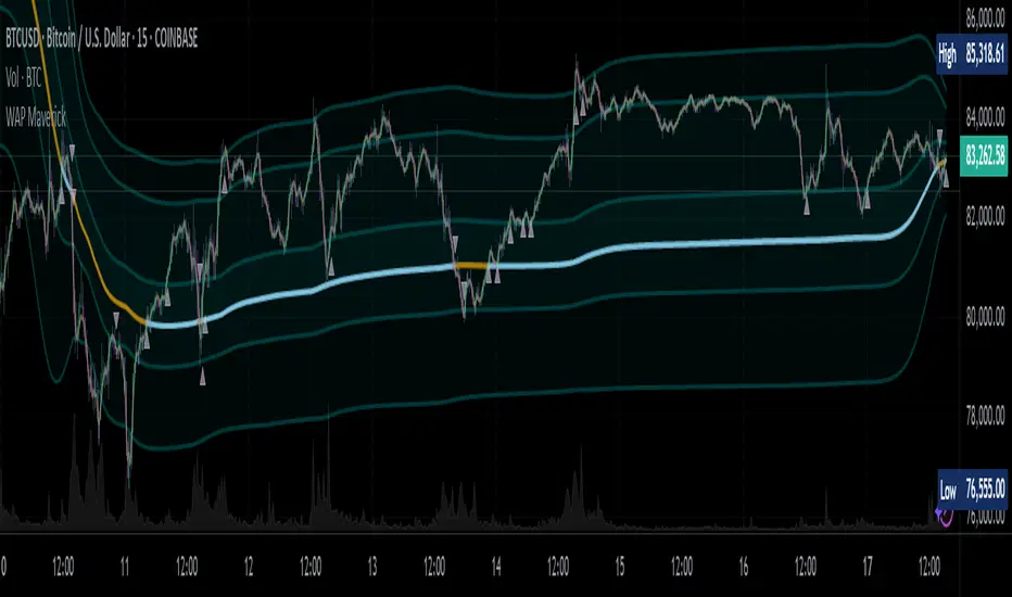
WAP Maverick - (Dual EMA Smoothed VWAP) - [mutantdog]Short Version:
This here is my take on the popular VWAP indicator with several novel features including:
Dual EMA smoothing.
Arithmetic and Harmonic Mean plots.
Custom Anchor feat. Intraday Session Sizes.
2 Pairs of Bands.
Side Input for Connection to other Indicator.
This can be used 'out of the box' as a replacement VWAP, benefitting from smoother transitions and easy-to-use custom alerts.
By design however, this is intended to be a highly customisable alternative with many adjustable parameters and a pseudo-modular input system to connect with another indicator. Well suited for the tweakers around here and those who like to get a little more creative.
I made this primarily for crypto although it should work for other markets. Default settings are best suited to 15m timeframe - the anchor of 1 week is ideal for crypto which often follows a cyclical nature from Monday through Sunday. In 15m, the default ema length of 21 means that the wap comes to match a standard vwap towards the end of Monday. If using higher chart timeframes, i recommend decreasing the ema length to closely match this principle (suggested: for 1h chart, try length = 8; for 4h chart, length = 2 or 3 should suffice).
Note: the use of harmonic mean calculations will cause problems on any data source incorporating both positive and negative values, it may also return unusable results on extremely low-value charts (eg: low-sat coins in /btc pairs).
Long version:
The development of this project was one driven more by experimentation than a specific end-goal, however i have tried to fine-tune everything into a coherent usable end-product. With that in mind then, this walkthrough will follow something of a development chronology as i dissect the various functions.
DUAL-EMA SMOOTHING
At its core this is based upon / adapted from the standard vwap indicator provided by TradingView although I have modified and changed most of it. The first mod is the dual ema smoothing. Rather than simply applying an ema to the output of the standard vwap function, instead i have incorporated the ema in a manner analogous to the way smas are used within a standard vwma. Sticking for now with the arithmetic mean, the basic vwap calculation is simply sum(source * volume) / sum(volume) across the anchored period. In this case i have simply applied an ema to each of the numerator and denominator values resulting in ema(sum(source * volume)) / ema(sum(volume)) with the ema length independent of the anchor. This results in smoother (albeit slower) transitions than the aforementioned post-vwap method. Furthermore in the case when anchor period is equal to current timeframe, the result is a basic volume-weighted ema.
The example below shows a standard vwap (1week anchor) in blue, a 21-ema applied to the vwap in purple and a dual-21-ema smoothed wap in gold. Notably both ema types come to effectively resemble the standard vwap after around 24 hours into the new anchor session but how they behave in the meantime is very different. The dual-ema transitions quite gradually while the post-vwap ema immediately sets about trying to catch up. Incidentally. a similar and slower variation of the dual-ema can be achieved with dual-rma although i have not included it in this indicator, attempted analogues using sma or wma were far less useful however.
STANDARD DEVIATION AND BANDS
With this updated calculation, a corresponding update to the standard deviation is also required. The vwap has its own anchored volume-weighted st.dev but this cannot be used in combination with the ema smoothing so instead it has been recalculated appropriately. There are two pairs of bands with separate multipliers (stepped to 0.1x) and in both cases high and low bands can be activated or deactivated individually. An example usage for this would be to create different upper and lower bands for profit and stoploss targets. Alerts can be set easily for different crossing conditions, more on this later.
Alongside the bands, i have also added the option to shift ('Deviate') the entire indicator up or down according to a multiple of the corrected st.dev value. This has many potential uses, for example if we want to bias our analysis in one direction it may be useful to move the wap in the opposite. Or if the asset is trading within a narrow range and we are waiting on a breakout, we could shift to the desired level and set alerts accordingly. The 'Deviate' parameter applies to the entire indicator including the bands which will remain centred on the main WAP.
CUSTOM (W)ANCHOR
Ever thought about using a vwap with anchor periods smaller than a day? Here you can do just that. I've removed the Earnings/Dividends/Splits options from the basic vwap and added an 'Intraday' option instead. When selected, a custom anchor length can be created as a multiple of minutes (default steps of 60 mins but can input any value from 0 - 1440). While this may not seem at first like a useful feature for anyone except hi-speed scalpers, this actually offers more interesting potential than it appears.
When set to 0 minutes the current timeframe is always used, turning this into the basic volume-weighted ema mentioned earlier. When using other low time frames the anchor can act as a pre-ema filter creating a stepped effect akin to an adaptive MA. Used in combination with the bands, the result is a kind of volume-weighted adaptive exponential bollinger band; if such a thing does not already exist then this is where you create it. Alternatively, by combining two instances you may find potential interesting crosses between an intraday wap and a standard timeframe wap. Below is an example set to intraday with 480 mins, 2x st.dev bands and ema length 21. Included for comparison in purple is a standard 21 ema.
I'm sure there are many potential uses to be found here, so be creative and please share anything you come up with in the comments.
ARITHMETIC AND HARMONIC MEAN CALCULATIONS
The standard vwap uses the arithmetic mean in its calculation. Indeed, most mean calculations tend to be arithmetic: sma being the most widely used example. When volume weighting is involved though this can lead to a slight bias in favour of upward moves over downward. While the effect of this is minor, over longer anchor periods it can become increasingly significant. The harmonic mean, on the other hand, has the opposite effect which results in a value that is always lower than the arithmetic mean. By viewing both arithmetic and harmonic waps together, the extent to which they diverge from each other can be used as a visual reference of how much price has changed during the anchored period.
Furthermore, the harmonic mean may actually be the more appropriate one to use during downtrends or bearish periods, in principle at least. Consider that a short trade is functionally the same as a long trade on the inverse of the pair (eg: selling BTC/USD is the same as buying USD/BTC). With the harmonic mean being an inverse of the arithmetic then, it makes sense to use it instead. To illustrate this below is a snapshot of LUNA/USDT on the left with its inverse 1/(LUNA/USDT) = USDT/LUNA on the right. On both charts is a wap with identical settings, note the resistance on the left and its corresponding support on the right. It should be easy from this to see that the lower harmonic wap on the left corresponds to the upper arithmetic wap on the right. Thus, it would appear that the harmonic mean should be used in a downtrend. In principle, at least...
In reality though, it is not quite so black and white. Rarely are these values exact in their predictions and the sort of range one should allow for inaccuracies will likely be greater than the difference between these two means. Furthermore, the ema smoothing has already introduced some lag and thus additional inaccuracies. Nevertheless, the symmetry warrants its inclusion.
SIDE INPUT & ALERTS
Finally we move on to the pseudo-modular component here. While TradingView allows some interoperability between indicators, it is limited to just one connection. Any attempt to use multiple source inputs will remove this functionality completely. The workaround here is to instead use custom 'string' input menus for additional sources, preserving this function in the sole 'source' input. In this case, since the wap itself is dependant only price and volume, i have repurposed the full 'source' into the second 'side' input. This allows for a separate indicator to interact with this one that can be used for triggering alerts. You could even use another instance of this one (there is a hidden wap:mid plot intended for this use which is the midpoint between both means). Note that deleting a connected indicator may result in the deletion of those connected to it.
Preset alertconditions are available for crossings of the side input above and below the main wap, alongside several customisable alerts with corresponding visual markers based upon selectable conditions. Alerts for band crossings apply only to those that are active and only crossings of the type specified within the 'crosses' subsection of the indicator settings. The included options make it easy to create buy alerts specific to certain bands with sell alerts specific to other bands. The chart below shows two instances with differing anchor periods, both are connected with buy and sell alerts enabled for visible bands.
Okay... So that just about covers it here, i think. As mentioned earlier this is the product of various experiments while i have been learning my way around PineScript. Some of those experiments have been branched off from this in order to not over-clutter it with functions. The pseudo-modular design and the 'side' input are the result of an attempt to create a connective framework across various projects. Even on its own though, this should offer plenty of tweaking potential for anyone who likes to venture away from the usual standards, all the while still retaining its core purpose as a traders tool.
Thanks for checking this out. I look forward to any feedback below.
Range Volume ChangeI was looking for a way to see if today's premarket volume is higher or lower than the previous day's premarket, but did not find any, hence, I made my own which I share with you now.
I call it 'Range Volume Change' or just RVC.
RVC will show the percentage of change between the selected time range and the previous day for the same time range.
This will allow us to see if the volume is increasing or decreasing today compared to the previous day by a specific time range that we set in PVC settings. It can do more than just premarket, you can use it for any time range of your interest which will work on 24hours assets like crypto and forex.
RVC visualizes the incremental of the volume using increasing size columns giving you a better view of how the volume changes compared to the past. The column shows the accumulated volume from when the time range started.
As an extra feature, it will also show the volume percentage of change outside the time range (can be disabled from settings).
In addition, RVC is also designed to work on real-time data.
Example of BTCUSDT (24-hour asset) with volume 'outside the time range', enabled (purple columns):
Follow for more awesome indicators/strategies: www.tradingview.com

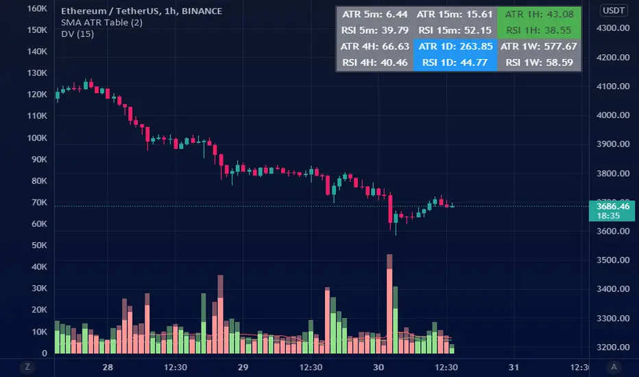
ATR Table (SMA)ATR table for select time frames.
Using Simple Moving Average (SMA) to get ATR.
MA periods is based on numbers suggested by Saeed Khakestar (Trigger Price Action)
You can change them in code
5m => 12
15m => 16
1H => 24
4H => 42
1D => 30
1W => 52
RSI is calculated the same way
SetSessionTimesLibrary "SetSessionTimes"
Function to automatically set session times for symbols and eventually timezone.
Useful mainly for futures contracts, to differentiate between pit and overnight sessions, and for 24 hours symbols if you want to "create" sessions for them
This library only returns correct session times to the calling script and does nothing by itself on the chart. the calling script must then use the returned session times to do anything.
For example, in the attached chart this library is used by my initial balance indicator, which calls it to retrieve the correct session times for the selected symbol in the chart, given that different futures contracts have different pit session times (RTH times) and Tradingview hasn't implemented that yet.
SetSessionTimes()

F&G_IndexIntroduction.
This indicator shows the behavior of Fear and Greed Index (F&G_Index) for the cryptocurrency market in an intuitive way for traders. This indicator has been modified from a script developed by @cptpat called "Fear and Greed Index FGI (Daily Update) alternative.me" (Tradingview user). The Fear and Greed Index values are taken directly from alternative.me.
The novelty of this proposal is to indicate the extreme levels (lower/upper) of the Fear and Greed Index according to a statistical analysis of the historical data. Also its daily update. It is not recommended to use in isolation. The appropriate way is in consensus with other indicators.
The extreme values.
Two upper and lower limits are established that correspond to the first standard deviation (1·SD) and 1.5 standard deviation (1.5·SD), respectively. These limits will help to know different important levels of greed or fear in the market based on real and historical data. The values obtained for each case are shown below, which will mark the extremes. These values may be modified in the future. If so, they will be updated and the community will be informed.
1·SD higher = 69 (F&G_Index).
1·SD lower = 24 (F&G_Index).
1.5·SD higher = 81 (F&G_Index).
1.5·SD lower = 12 (F&G_Index).
These limits are statistically significant and representative of extreme values of the Fear and Greed Index. Above all, for the case of 1.5·SD higher/lower, whose occurrence of the cases are significantly lower. These data are obtained for a daily record from August 2017 to December 2021, for a total of 1407 data. The occurrence of the Fear and Greed Index value exceeding the indicated levels is shown below.
F&G_Index > 1·SD higher (Greed). Occurrence <22,5%
F&G_Index < 1·SD lower (Fear). Occurrence <19%
1·SD lower < F&G_Index < 1·SD higher (Neutral). Occurrence ≈59%
F&G_Index > 1.5·SD higher (Extreme Greed). Occurrence <8%
F&G_Index < 1.5·SD lower (Extreme Fear). Occurrence <3%
How to use the indicator.
Its use is very simple and intuitive and is based on the levels indicated above. The blue line shows the historical value of F&G_Index. When the value of F&G_Index exceeds the levels indicated above, a vertical band of color will be tinted (brown/red, green/lime green or gray with transparency) as indicated below. This allows you to locate important areas in a very visual way.
F&G_Index > 1·SD higher (Greed). Brown color
F&G_Index < 1·SD lower (Fear). Green color.
1·SD lower < F&G_Index < 1·SD higher (Neutral). Gray color with transparency.
F&G_Index > 1.5·SD higher (Extreme Greed). Red color.
F&G_Index < 1.5·SD lower (Extreme Fear). Lime green color.
Image of the indicator.
